1 lecture 1 { elements of set theory and mathematical...
TRANSCRIPT
University of Leipzig – WS18/1910-PHY-BIPMA1 – Mathematics 1 / Vitalii Konarovskyi
The lecture notes are based on the following literature:
• A.Y. Dorogovtsev, Mathematical analysis, Kyiv, Fact, 2004, (Russian).
• K.A. Ross, Elementary analysis: The theory of calculus, Undergraduate Texts in Mathematics,Springer New York, 2013.
• I. Lankham, B. Nachtergaele, and A. Schilling, Linear algebra as an introduction to abstractmathematics, WSPC, 2016.
• B. P. Demidovic, Problems and exercises in mathematical analysis, Moscow, 1997, (Russian).
1 Lecture 1 – Elements of Set Theory and Mathematical Induction
1.1 Elements of Set Theory
The notion of a set is one of the most important initial and nondefinable notions of the modernmathematics. By a “set” we will understand any collection into a whole M of definite and separateobjects m of our intuition or our thought (Georg Cantor). These objects are called the “elements” ofM . Shortly we will use the notation m ∈ M or M 3 m. The fact that m does not belong to M isdenoted by m 6∈M .
A set M can be defined by listing of its elements. For instance,
• N = {1, 2, 3, . . . , n, . . .} — the set of natural numbers;
• Z = {. . . ,−n, . . . ,−1, 0, 1, 2, 3, . . . , n, . . .} — the set of integer numbers.
A set also can be defined by specifying of properties of its elements. In any mathematical problemusually consider elements of some quite defined set X. The needed set can be chosen by some propertyP satisfying the following property: for each x from X either x satisfies P (in this case one writesP (x)) or x does satisfy it. This set is denoted by {x ∈ X : P (x)} or {x : P (x)}. The set which doesnot contain any elements is called empty and is denoted ∅.
Example 1.1. 1. N = {n ∈ Z : n > 0}. Here P means “to be positive”, which is satisfied by anyinteger number.
2. Let P denote “to be even”. Then {2, 4, . . . , 2k, . . .} = {n ∈ N : P (n)}.
3. Q ={mn : n ∈ N, m ∈ Z
}. This is the set of rational numbers.
Exercise 1.1. List elements of the following sets:
a) {n ∈ N : (n− 3)2 < 72};
b){n ∈ N : n2+3n−12
n ∈ N}
;
c){n ∈ N : n+9
n+1 ∈ N}
;
d){n ∈ Z : n3 > 10n2
}.
1
University of Leipzig – WS18/1910-PHY-BIPMA1 – Mathematics 1 / Vitalii Konarovskyi
1.1.1 Operations on Sets
Let A and B be sets.
Definition 1.1. A set A is a a subset of a set B, if each element x of A is an element of B (orshortly, ∀x ∈ A ⇒ x ∈ B). Notation: A ⊂ B.
Definition 1.2 (Operations on sets). • A∪B = {x : x ∈ A or x ∈ B}— the union of A and B;
• A ∩B = {x : x ∈ A and x ∈ B} — the intersection of A and B;
• A \B = {x : x ∈ A and x 6∈ B} — the difference of A and B;
• A4B = {x : x ∈ A ∪B and x 6∈ A ∩B} — the symmetric difference of A and B;
• Ac = {x ∈ X : x 6∈ A} — the complement of A, where X is some given set containing A.
Exercise 1.2. Show that
a) A ∪ ∅ = A, A ∪A = A, A ∪B = B ∪A, A ∪ (B ∪ C) = (A ∪B) ∪ C =: A ∪B ∪ C;
b) A ∩ ∅ = ∅, A ∩A = A, A ∪B = B ∩A, A ∩ (B ∩ C) = (A ∩B) ∩ C =: A ∩B ∩ C;
c) A4B = (A ∪B) \ (A ∩B) = (A \B) ∪ (B \A), A \B = A ∩Bc;
d) A ∩ (B ∪ C) = (A ∩B) ∪ (A ∩ C), A ∪ (B ∩ C) = (A ∪B) ∩ (A ∪ C).
e) (A ∪B)c = Ac ∩Bc, (A ∩B)c = Ac ∪Bc.
Let T be a set of indexes and for each t ∈ T a set At is given.
Definition 1.3. • ⋃t∈T
At = {x : ∃t0 ∈ T At0 3 x} — the union of the family At, t ∈ T ;
• ⋂t∈T
At = {x : ∀t ∈ T At 3 x} — the intersection of the family At, t ∈ T ;
Example 1.2. Let An = {1, . . . , n} for each n ∈ N. Then
⋃n∈N
An =∞⋃n=1
An = N,⋂n∈N
An =∞⋂n=1
An = {1}.
1.2 Numbers
1.2.1 Mathematical induction
For more details see [1, Section 1.1].Let M be a subset of natural numbers which satisfies the following properties
1) 1 ∈M ;
2) if n ∈M , then n+ 1 ∈M .
Then M = N! This is one of the axioms of natural numbers and it is the basis of mathematicalinduction. Let P1, P2, P3, . . . be a list of statements or propositions that may or may not be true.The principle of mathematical induction asserts all the statements P1, P2, P3, . . . are true provided
2
University of Leipzig – WS18/1910-PHY-BIPMA1 – Mathematics 1 / Vitalii Konarovskyi
(I1) P1 is true;
(I2) Pn+1 is true whenever Pn is true.
We will refer to (I1) as the basis for induction and we will refer to (I2) as the induction step.
Example 1.3. Prove 1 + 2 + · · ·+ n = 12n(n+ 1) for positive integers n.
Solution. Our n-th proposition is
Pn : 1 + 2 + · · ·+ n =1
2n(n+ 1).
Base case: Show that the statement Pn holds for n = 1. So,
1 =1
2· 1 · (1 + 1).
Induction step: We assume that Pn holds, i.e.
1 + 2 + · · ·+ n =1
2n(n+ 1)
is true, and must prove Pn+1. So,
1 + 2 + · · ·+ n+ (n+ 1) =1
2n(n+ 1) + (n+ 1) =
1
2(n+ 1)(n+ 2) =
1
2(n+ 1)((n+ 1) + 1).
By the principle of mathematical induction, we conclude that Pn is true for all n.
Exercise 1.3. a) Prove that all numbers of the form 5n − 4n− 1, n ∈ N are divisible by 16.
b) Show that 13 + 23 + . . .+ n3 = (1 + 2 + . . .+ n)2 for each n ∈ N.
c) Prove the inequality 1 + 122
+ . . .+ 1n2 ≤ 2− 1
n for all n ∈ N.
3
University of Leipzig – WS18/1910-PHY-BIPMA1 – Mathematics 1 / Vitalii Konarovskyi
2 Lecture 2 – Completeness of the Set of Real Numbers and someInequalities
2.1 Real Numbers
2.1.1 Definition of Real Numbers
Very often the set of rational numbers needs an extension. For example, the length of a diagonal of asquare with side 1 can not be given as a rational number.
Exercise 2.1. Prove that there does not exist a rational number x solving the equation x2 = 2.
Definition 2.1. A real number is an infinite sequence of numerical digits with the comma betweenthem, that is,
a = α0, α1α2 . . . αn . . . ,
where α0 ∈ Z and αn ∈ {0, 1, . . . , 9} for all n ∈ N.
The set of all real numbers is denoted by R.
Definition 2.2. Numbers from R \Q is called irrational.
Remark 2.1. We will identify of two real numbers of the form
a = α0, α1 . . . αn99999 . . .
anda = α0, α1 . . . (αn + 1)00000 . . . ,
where αn < 9. Further, we will avoid numbers, where 9 is in the period.
The order relations “<,≤, >,≥” between real numbers can be introduced by the natural way aswell as the notions of positive and negative real numbers.
Definition 2.3. The absolute value of a real number a is defined as follows
|a| ={a, if a ≥ 0,
−a, if a < 0.
2.1.2 Supremum and Infimum of Subsets of Real Numbers
Let A be a non-empty subset of R.
Definition 2.4. • If A contains a larger element a0, then we call a0 the maximum of A andwrite a0 = maxA.
• If A contains a smallest element, then we call the smallest element the minimum of A and writeit as minS.
Example 2.1. a) max{1, 2, 3, 4, 5} = 5, min{1, 2, 3, 4, 5} = 1;
b) Let A ={
1n : n ∈ N
}. Then maxA = 1 but minA does not exist.
4
University of Leipzig – WS18/1910-PHY-BIPMA1 – Mathematics 1 / Vitalii Konarovskyi
Definition 2.5. • If a real number M satisfies a ≤ M for all a ∈ A, then M is called an upperbound of A and the set A is said to be bounded above.
• If a real number m satisfies m ≤ a for all a ∈ A, then m is called a lower bound of A and theset A is said to be bounded below.
• The set A is said to be bounded if it is bounded above and bounded below.
Example 2.2. 1. The set A ={
1n : n ∈ N
}is bounded.
2. The set N is bounded below but not above.
3. The set R is neither bounded below nor above.
Exercise 2.2. Prove that the following sets are bounded:
a){
nn+1 : n ∈ N
};
b){
(−1)nn+1n−(−1)n : n ∈ N
}.
Definition 2.6. • If A is bounded above and A has a least upper bound, then we will call it thesupremum of A and denote it by supA.
• If A is bounded below and A has a greatest lower bound, then we will call it the infimum of Aand denote it by inf A.
Exercise 2.3. If minA exists, then minA = inf A. Similarly, if maxA exists, then maxA = supA.Check these statements.
Theorem 2.1. (i) The number a∗ is the supremum of a subset A of R iff
• a∗ is an upper bound of A;
• ∀a < a∗ ∃x ∈ A x > a.
(ii) The number a∗ is the supremum of a subset A of R iff
• a∗ is an lower bound of A;
• ∀a > a∗ ∃x ∈ A x < a.
Exercise 2.4. For each a < b prove that inf[a, b] = inf(a, b] = a and sup[a, b] = sup[a, b) = b.
Theorem 2.2. (i) For every non-empty subset A of R that is bounded above supA exists and is areal number.
(ii) For every non-empty subset A of R that is bounded below inf A exists and is a real number.
The latter theorem states the completeness of the set of real numbers, which is not true e.g. forrational numbers. Indeed, the set A = {r ∈ Q : 0 ≤ r and r2 ≤ 2} is a set of rational numbers and it isbounded above by some rational numbers but A has no least upper bound that is a rational number.
5
University of Leipzig – WS18/1910-PHY-BIPMA1 – Mathematics 1 / Vitalii Konarovskyi
Theorem 2.3. For each positive real number a = α0, α1α2 . . . αn . . ., we have
a = sup{an : n ∈ N},
where an = α0, α1α2 . . . αn.
Exercise 2.5. Prove Theorem 2.3.
Now, we are ready to introduce operation or real numbers. Let a, b be a positive real numbers andan and bn, n ∈ N, be defined as in Theorem 2.3.
Definition 2.7. We set by the definition a+ b := sup{an + bn : n ∈ N}; a · b := sup{an · bn : n ∈ N};ab := sup
{anbn
: n ∈ N}
; for a > b, a− b := sup{an − bn : n ∈ N}.
We note that all numbers an and bn, n ∈ N, in the definition are rational and for them all arithmeticoperations are defined. All known properties of arithmetic operations on integer numbers are also validfor real numbers but now they have to be proved.
Exercise 2.6. Show that
a) a · b = b · a and a+ b = b+ a;
b) a+ (b+ c) = (a+ b) + c =: a+ b+ c
c) a · (b · c) = (a · b) · c =: a · b · c.
2.1.3 n-th Root of a Positive Real Number
Theorem 2.4. Let a be a positive real number and n ∈ N. Then there exist a unique positive realnumber x satisfying xn = a, where xn := x · . . . · x︸ ︷︷ ︸
n times
.
Remark 2.2. The number x can be constructed as the supremum of the set {y > 0 : yn < a}, whichis a non-empty bounded above set.
Definition 2.8. Let a > 0 and n ∈ N. The unique positive solution of the equation xn = a, whichexists according to Theorem 2.4, is called the n-th root of the positive real number a. We use thenotation for x: a
1n = n
√a.
Definition 2.9. Let a > 0 and r ∈ Q, r > 0. We define
ar := (am)1n ,
where r = mn , m,n ∈ N.
Definition 2.10. Let a > 1 and b > 0. We define
ab := sup{abn : n ∈ N},
where b := β0, β1β2 . . . βn . . . and bn := β0, β1β2 . . . βn.
Exercise 2.7. Give a definition of ab in the case 0 < a < 1 and b > 0.
6
University of Leipzig – WS18/1910-PHY-BIPMA1 – Mathematics 1 / Vitalii Konarovskyi
2.2 Some important inequalities
We recall that the absolute value of a real number a is given by
|a| ={a, if a ≥ 0,
−a, if a < 0.
We note that −|a| ≤ a ≤ |a| and also |a| < c ⇔ −c < a < c. Moreover, |a| = | − a|.
Theorem 2.5. For all a, b ∈ R the inequalities
1) |a+ b| ≤ |a|+ |b| 2) ||a| − |b|| ≤ |a− b|
holds. For every a1, . . . an ∈ R one has
|a1 + . . .+ an| ≤ |a1|+ . . .+ |an|.
Proof. Since −|a| ≤ a ≤ |a| and −|b| ≤ b ≤ |b|, we obtain −(|a|+ |b|) ≤ a+ b ≤ |a|+ |b|. This impliesinequality 1). Now, applying 1), we obtain |a| = |a− b + b| ≤ |a− b|+ |b|. Hence, |a| − |b| ≤ |a− b|.Since |a− b| = |b− a| ≥ |b| − |a|, we obtain 2). The latter inequality trivially follows from 1).
Inequality 1) from Theorem 2.5 is called the triangular inequality.
Theorem 2.6 (Bernoulli’s inequality). For each real number x > −1 and n ∈ N the inequality
(1 + x)n ≥ 1 + nx
holds. Moreover, (1 + x)n = 1 + nx iff x = 0 or n = 1.
Proof. If n = 1 or x = 0, then the equality holds. We assume that x 6= 0 and use mathematicalinduction to prove (1 + x)n > 1 + nx for all n ≥ 2. So, for n = 2 one has
(1 + x)2 = 1 + 2x+ x2 > 1 + 2x.
Next, we assume that the strict inequality holds for some n ≥ 2. Then
(1 + x)n+1 = (1 + x)(1 + x)n > (1 + x)(1 + nx) = 1 + (n+ 1)x+ nx2 > 1 + (n+ 1)x.
Exercise 2.8. Show thata) 2n ≥ n+ 1, n ∈ N; b) 3n ≥ 2n+ 1, n ∈ N; c) 2n > (
√2− 1)2n2, n ∈ N.
Exercise 2.9. Let x1, . . . , xn be a positive real numbers. Prove that
(1 + x1) · . . . · (1 + xn) ≥ 1 + x1 + . . .+ xn.
7
University of Leipzig – WS18/1910-PHY-BIPMA1 – Mathematics 1 / Vitalii Konarovskyi
3 Lecture 3 – Convergence of Sequences
3.1 Limits of Sequences
For more details see [1, Section 2.7].In this section, we will study some properties of sequences of real numbers which do not depend on
finite numbers of their elements. So, we will call a sequence any enumerated collection of objects (inour case, real numbers) in which repetitions are allowed. It is often convenient to write the sequenceas (am, am+1, am+2, . . .), (an)n≥m or (an)∞n=m, where m is some integer number. Usually, m equals 1.
Definition 3.1. A sequence (an)n≥1 = (a1, a2, . . . , an, . . .) is called bounded if there exists C > 0such that |an| ≤ C for all n ≥ 1. In another words, if all elements of the sequence belong to someinterval [−C,C].
Example 3.1. 1. The sequence ((−1)n)n≥1 = (−1, 1,−1, 1, . . .) is bounded and its elements belongto [−1, 1];
2. The sequence (sinn)n≥1 is bounded and its elements also belong to [−1, 1];
3. The sequence (n)n≥1 = (1, 2, 3, . . . , n, . . .) is unbounded, since for each C > 0 one can find anumber n ∈ N larger than C.
Exercise 3.1. Prove the boundedness of the following sequences:
a)(2n
n!
)n≥1; b)
an =
√2 +
√2 + . . .+
√2 +√
2︸ ︷︷ ︸n square roots
n≥1
;
c)(an = 1 + 2
2 + 322
+ . . .+ n2n−1
)n≥1 (Hint: Use the equality 1
2an = an − 1
2an)
Exercise 3.2. Prove that a sequence (an)n≥1 is bounded iff (a3n − an)n≥1 is bounded.
Definition 3.2. Let x ∈ R and ε > 0 be given. A neighbourhood or ε-neighbourhood of thepoint x is the interval (x− ε, x+ ε) = {y ∈ R : |y − x| < ε}.
Exercise 3.3. Check that: a) intersection of a finite number of neighbourhoods of x is again aneighbourhood of x; b) intersection of two neighbourhoods is either ∅ or a neighbourhood.
Definition 3.3. A sequence (an)n≥1 of real numbers is said to converge to a real number a providedthat
for each ε > 0 there exists a number N such that n ≥ N implies |an − a| < ε,
or, shortly,∀ε > 0 ∃N ∈ R ∀n ≥ N : |an − a| < ε.
If (an)n≥1 converges to a, we will write limn→∞
an = a or an → a, n → ∞. The number a is called
the limit of the sequence (an)n≥1. A sequence that does not converge to some real number is said todiverge.
Remark 3.1. We note that an → a, n→∞, provided that any ε-neighbourhood of point a containselements an for all n ≥ N , where N is some number depending on ε.
8
University of Leipzig – WS18/1910-PHY-BIPMA1 – Mathematics 1 / Vitalii Konarovskyi
Exercise 3.4. For which sequences (an)n≥1 the number N from Definition 3.3 could be taken inde-pendent of ε.
Answer: If ∃m ∈ N ∀n ≥ m : an = a.
Exercise 3.5. Prove the following statements:
a) an → a, n→∞ ⇔ an − a→ 0, n→∞ ⇔ |an − a| → 0, n→∞;
b) an → 0, n→∞ ⇔ |an| → 0, n→∞;
c) an → a, n→∞ ⇔ ∀ε > 0 ∃N ∈ N : {aN , aN+1, . . .} ⊂ (x− ε, x+ ε);
d) an → 0, n→∞ ⇔ sup{|ak| : k ≥ n} → 0, n→∞;
e) an → a, n→∞ ⇒ |an| → |a|, n→∞.
Theorem 3.1. A sequence can have only a unique limit.
Proof. Let an → a, n→∞, and an → b, n→∞. Then by the definition, ∀ε > 0 ∃N1 ∈ R ∀n ≥ N1 :|an − a| < ε and ∀ε > 0 ∃N2 ∈ R ∀n ≥ N2 : |an − b| < ε. Thus, using the triangular inequality (seeTheorem 2.5 1)), we obtain ∀ε > 0 ∀n ≥ max{N1, N2} : |a−b| = |a−an+an−b| ≤ |a−an|+|an−b| <2ε. So, |a− b| < 2ε for all ε > 0. If a 6= b, we set ε = |a−b|
3 > 0. Then |a− b| < 23 |a− b| ⇒ 1
3 |a− b| < 0,that is impossible.
3.2 Some Examples
For more examples see [1, Section 2.8].
Theorem 3.2. The equality limn→∞
1n = 0 holds.
Proof. We note that for each ε > 0 we have∣∣ 1n − 0
∣∣ = 1n < ε iff n > 1
ε . Thus, ∀ε > 0 ∃N :=(1ε + 1
)∈
R ∀n ≥ N :∣∣ 1n − 0
∣∣ < ε.
Corollary 3.1. The equality limn→∞
1nα = 0 holds for each α > 0.
Theorem 3.3. Let a ∈ R, |a| > 1, b ∈ R. Then limn→∞
nb
an = 0.
Proof. We choose k ∈ N such that k ≥ b + 1. By Bernoulli’s inequality (see Theorem 2.6), |a|n =(|a|nk
)k=((
1 +(|a| 1k − 1
))n)k> nk
(|a| 1k − 1
)k. Hence,
∣∣∣nban − 0∣∣∣ = nb
|a|n ≤ nk−1
|a|n < 1
n
(|a|
1k−1
)k < ε.
So, n > 1
ε
(|a|
1k−1
)k . Consequently, one can claim
∀ε > 0 ∃N :=1
ε(|a| 1k − 1
)k + 1 ∀n ≥ N :
∣∣∣∣nban − 0
∣∣∣∣ < ε.
Theorem 3.4. The equality limn→∞
n√n = 1 holds.
9
University of Leipzig – WS18/1910-PHY-BIPMA1 – Mathematics 1 / Vitalii Konarovskyi
Proof. By Exercise 3.5 a), it is enough to show that an := n√n − 1 → 0, n → ∞. Since (1 + an)n =
( n√n)n = n, one has
n = (1 + an)n ≥ 1 + nan +1
2n(n− 1)a2n >
1
2n(n− 1)a2n,
by the binomial formula. Thus, an <√
2n−1 for n ≥ 2. Next using the standard argument, one has
an → 0.
Exercise 3.6. Check the following equalities:a) lim
n→∞an = 0 for all 0 < a < 1; b) lim
n→∞n√a = 1 for all a > 0; c) lim
n→∞lgnnα = 0 for all α > 0, where
lg := log10.
Definition 3.4. 1. limn→∞
an = +∞ ⇔ ∀C ∈ R ∃N ∈ R ∀n ≥ N : an ≥ C.
2. limn→∞
an = −∞ ⇔ ∀C ∈ R ∃N ∈ R ∀n ≥ N : an ≤ C.
Exercise 3.7. Prove that for a sequence (an)n≥1 with an 6= 0 the equality limn→∞
|an| = +∞ is equivalent
to limn→∞
1an
= 0.
Exercise 3.8. Let (an)n≥1 be a sequence such that ann → 0, n→∞. Prove that max{a1,a2,...,an}
n → 0,n→∞.
Exercise 3.9. Assume that an → a, n → ∞, and bn → b, n → ∞. Show that max{an, bn} →max{a, b}, n→∞.
3.3 Limit Theorems for Sequences
See also [1, Section 2.9].In this section, we will prove some properties of convergent sequences and their limits. We recall
that a sequence (an)n≥1 of real numbers is said to be bounded if there exists a constant C such that|an| ≤ C for all n.
Theorem 3.5. Any convergent sequence is bounded.
Proof. Let an → a, n→∞. We have to show that (an)n≥1 is bounded. By the definition of convergence(see Definition 3.3), for each ε > 0, in particular for ε = 1, there exists a number N , which can be takenfrom N, such that |an − a| < ε = 1 for all n ≥ N . Thus, setting C := max{|a1|, . . . , |aN−1|, |a| + 1},one trivially obtains for n ∈ {1, 2, . . . , N − 1}
|an| ≤ C.
Next, using the triangular inequality (inequality 1) of Theorem 2.5), we have
|an| = |an − a+ a| ≤ |an − a|+ |a| < 1 + |a| ≤ C,
for all n ≥ N .
Exercise 3.10. Give an example of a bounded divergent sequence.
10
University of Leipzig – WS18/1910-PHY-BIPMA1 – Mathematics 1 / Vitalii Konarovskyi
Theorem 3.6. Let an → a, n→∞, bn → b, n→∞, and let an ≤ bn for all n ≥ 1. Then a ≤ b.
Exercise 3.11. Prove Theorem 3.6.
Remark 3.2. We note that replacing the inequality an ≤ bn by the strong one, i.e. an < bn, it doesnot imply a < b. Indeed, for an := 0 and bn := 1
n , n ≥ 1, one has an < bn but an → 0, bn → 0, n→∞.
Remark 3.3. Theorem 3.6 remains valid, if the inequality an ≤ bn holds only for all n ≥ M , whereM is some number N .
Theorem 3.7 (Squeeze theorem). Let sequences (an)n≥1, (bn)n≥1 and (cn)n≥1 satisfy the followingconditions:
a) an ≤ bn ≤ cn for all n ≥ 1;
b) an → a, n→∞, and cn → a, n→∞.
Then bn → a, n→∞.
Proof. We prove the theorem only for the case a ∈ R. According to Remark 3.1, for each ε > 0 thereexists N1 and N2 from R such that an belongs to the ε-neighbourhood (a− ε, a+ ε) of the point a forall n ≥ N1 and cn belongs to (a− ε, a+ ε) for all n ≥ N2. Thus, for all n ≥ max{N1, N2} elements bnalso belong to (a− ε, a+ ε) due to property a).
Example 3.2. Show that limn→∞
n
√1 + 1
2 + 13 + . . .+ 1
n = 1.
Solution. We take an := n√
1 = 1 and cn := n√
1 + 1 + 1 + . . .+ 1︸ ︷︷ ︸n times
= n√n. Then
an ≤ n
√1 +
1
2+
1
3+ . . .+
1
n≤ cn
for all n ≥ 1. Moreover, an → 1, n→∞, and cn → 1, n→∞, by Theorem 3.4. Hence, Theorem 3.7
implies limn→∞
n
√1 + 1
2 + 13 + . . .+ 1
n = 1.
Theorem 3.8. Let an → a ∈ R, n→∞, and bn → b ∈ R, n→∞. Then
a) limn→∞
(c · an) = c · limn→∞
an for all c ∈ R;
b) limn→∞
(an + bn) = limn→∞
an + limn→∞
bn;
c) limn→∞
(an · bn) = limn→∞
an · limn→∞
bn;
d) limn→∞
anbn
=limn→∞
an
limn→∞
bn, if b 6= 0.
Proof. For proof of the theorem see Section 2.9 [1].
11
University of Leipzig – WS18/1910-PHY-BIPMA1 – Mathematics 1 / Vitalii Konarovskyi
Example 3.3. Compute the limit limn→∞
2n2+lgn3n2+n cosn+5
.
Solution. We cannot apply Theorem 3.8 directly, since the numerator and denominator of 2n2+lgn3n2+n cosn+5
tend to infinity. So, first we rewrite them as follows:
2n2 + lg n
3n2 + n cosn+ 5=
n2 ·(
2 + lgnn2
)n2 ·
(3 + cosn
n + 5n2
) =2 + lgn
n2
3 + cosnn + 5
n2
.
Now, we can use Theorem 3.8 d) to the right hand side of the latter equality. Indeed, we first compute
limn→∞
(2 +
lg n
n2
)= 2 + lim
n→∞
lg n
n2= 2,
by, Theorem 3.8 b) and Exercise 3.6 c). Next, due to the inequality
− 1
n≤ cosn
n≤ 1
n, n ≥ 1,
theorems 3.7 and 3.2, one has limn→∞
cosnn = 0. Thus, by Theorem 3.8 a), b)
limn→∞
(3 +
cosn
n+
5
n2
)= 3 + lim
n→∞
cosn
n+ 5 lim
n→∞
1
n2= 3 6= 0.
So, we can apply Theorem 3.7 d) and obtain
limn→∞
2n2 + lg n
3n2 + n cosn+ 5= lim
n→∞
2 + lgnn2
3 + cosnn + 5
n2
=2
3.
Exercise 3.12. Compute the following limits:a) lim
n→∞sin2 n√
n; b) lim
n→∞n2+sinnn2+n cosn
; c) limn→∞
n√n22n + 3n; d) lim
n→∞2n+n3
3n+1 ; e) n+1√n.
Exercise 3.13. Let (an)n≥1 be a bounded sequence and bn → 0, n ≥ ∞. Prove that anbn → 0,n→∞.
Exercise 3.14. Let (an)n≥1 be a bounded sequence and bn → +∞, n ≥ ∞. Prove that an+bn → +∞,n→∞.
Exercise 3.15. Let an ≥ 0 for all n ≥ 1 and an → a, n → ∞. Show that for all k ∈ N one hask√an → k
√a, n→∞.
Exercise 3.16. Let an → a ∈ R, n→∞. Prove that a1+...+ann → a, n→∞.
12
University of Leipzig – WS18/1910-PHY-BIPMA1 – Mathematics 1 / Vitalii Konarovskyi
4 Lecture 4 – Subsequences and Monotone Sequences
4.1 Monotone Sequences
The main goal of this section is to prove that any bounded monotone sequence must converge. So, westart from the definition.
Definition 4.1. A sequence (an)n≥1 of real numbers is called an increasing sequence if an ≤ an+1
for all n ≥ 1, and (an)n≥1 is called a decreasing sequence if an ≥ an+1 for all n ≥ 1. A sequencethat is increasing or decreasing is said to be a monotone sequence.
Example 4.1. The sequence (1, 1, 2, 2, 3, 3, 4, 4, . . .) is increasing, but (−1, 1,−1, 1, . . .) is not mono-tone.
Exercise 4.1. a) Show that any bounded above increasing sequence is bounded. b) Show that anybounded below decreasing sequence is bounded.
Exercise 4.2. a) Prove that (n2−n)n≥2 is a decreasing sequence.
b) Let (an)n≥1 be an increasing sequence of positive numbers and define σn = a1+...+ann . Prove that
(σn)n≥1 is also an increasing sequence.
Theorem 4.1. Every bounded monotone sequence converges.
Proof. We will prove the theorem for increasing sequences. The case of decreasing sequences is leftto Exercise 4.3. So, let a sequence (an)n≥1 increase. By the assumption of the theorem, (an)n≥1 isbounded, that is, there exists C ∈ R such that |an| ≤ C for all n ≥ 1. This implies that the setA := {an : n ≥ 1} is also bounded. Thus, by Theorem 2.2 (i) there exists supA =: sup
n≥1an denoted by
a. Let us prove that an → a, n→∞. We first note that an ≤ a for all n ≥ 1, since the supremum of Ais also its upper bound (see Definition 2.6). Next, we take an arbitrary ε > 0 and use Theorem 2.1 (i).So, there exists a number m such that am > a − ε. By the monotonicity, a − ε < am ≤ an for alln ≥ m. Thus, setting N := m, one has a− ε < an ≤ a for all n ≥ N which implies |an − a| < ε.
Exercise 4.3. Prove Theorem 4.1 for decreasing sequences.
Remark 4.1. Theorem 4.1 remains valid if one requires the monotonicity of (an)n≥1 starting fromsome number m, that is, the monotonicity of (an)n≥m = (am, am+1, . . .).
Example 4.2. Prove that limn→∞
10n
n! = 0, where n! := 1 · 2 · 3 · . . . · n.
Solution. First we note that 10n+1
(n+1)! <10n
n! ⇔ 10 < n+ 1 ⇔ n > 9. Hence, the sequence(10n
n!
)n≥10
is decreasing. Moreover, it is bounded below by zero. Thus,(10n
n!
)n≥10 is bounded, by Exercise 4.1 b).
Using Theorem 4.1, one gets that there exists a ∈ R such that limn→∞
10n
n! = a. But we can write
10n+1
(n+1)! = 10n
n! · 10n+1 . So,
a = limn→∞
10n+1
(n+ 1)!= lim
n→∞
10n
n!· limn→∞
10
n+ 1= a · 0.
This implies a = 0.
13
University of Leipzig – WS18/1910-PHY-BIPMA1 – Mathematics 1 / Vitalii Konarovskyi
Exercise 4.4. Show that a) limn→∞
n!
2n2= 0; b) lim
n→∞n
2√n = 0.
Exercise 4.5. Find a limit of the sequence
(√2,√
2 +√
2,
√2 +
√2 +√
2, . . .
).
Exercise 4.6. Let a1 = 1 and an+1 = 13(an + 1) for all n ≥ 1.
a) Find a2, a3, a4.
b) Use induction to show that an >12 for all n ≥ 1.
c) Show that (an)n≥1 is a decreasing sequence.
d) Show that limn→∞
an exists and find it.
Exercise 4.7. Let c > 0, a1 > 0 and let an+1 = 12
(an + c
an
)for all n ≥ 1.
a) Show that an ≥√c for all n ≥ 2.
b) Show that (an)n≥2 is a decreasing sequence.
c) Show that limn→∞
an exists and find it.
Theorem 4.2. (i) If (an)n≥1 is an unbounded increasing sequence, then limn→∞
an = +∞.
(ii) If (an)n≥1 is an unbounded decreasing sequence, then limn→∞
an = −∞.
Proof. We will prove only Part (i) of the theorem. The proof of Part (ii) is similar. If (an)n≥1 isan unbounded increasing sequence, then it must be unbounded above, since it is bounded below bya1. Taking any C and using the unboundedness of (an)n≥1, one can find a number m ∈ N such thatam ≥ C. Next, by the monotonicity of (an)n≥1, the inequality an ≥ am ≥ C trivially holds for alln ≥ N := m. This proves lim
n→∞an = +∞ (see Definition 3.4).
Corollary 4.1. If (an)n≥1 is a monotone sequence, then the sequence either converges, diverges to+∞, or diverges to −∞. Thus lim
n→∞an is always meaningful for monotone sequences.
Proof. The proof immediately follows from theorems 4.1 and 4.2.
Exercise 4.8. Let A be a bounded nonempty subset of R such that supA is not in A. Prove thatthere is an increasing sequence (an)n≥1 of points from A such that lim
n→∞an = supA.
4.2 The number e
In this section, we will consider two sequences of positive numbers(an :=
(1 +
1
n
)n)n≥1
and
(bn :=
(1 +
1
n
)n+1)n≥1
(1)
and study their properties.
14
University of Leipzig – WS18/1910-PHY-BIPMA1 – Mathematics 1 / Vitalii Konarovskyi
Theorem 4.3. The sequences defined in (1) satisfy the following properties:
1) an < bn for all n ≥ 1;
2) the sequence (an)n≥1 increases;
3) the sequence (bn)n≥1 decreases.
Proof. Since bn = an(1 + 1
n
)= an + an
n > an for all n ≥ 1, Property 1) is proved.To prove 2), we are going to use Bernoulli’s inequality (see Theorem 2.6). So, one has
anan−1
=
(n+ 1
n
)n(n− 1
n
)n−1=
n
n− 1
(1− 1
n2
)n>
n
n− 1
(1− n
n2
)= 1,
for all n ≥ 2. Thus, an > an−1 for all n ≥ 2.For the prove of 3) we use the same argument. We consider
bn−1bn
=
(n
n− 1
)n( n
n+ 1
)n+1
=n− 1
n
(n2
n2 − 1
)n+1
=n− 1
n
(1 +
1
n2 − 1
)n+1
>n− 1
n
(1 +
n+ 1
n2 − 1
)= 1,
for all n ≥ 2. Hence, bn−1 > bn for all n ≥ 2.
Theorem 4.3 yields the following inequalities
a1 < a2 < . . . < an < . . . < bn < . . . < b2 < b1. (2)
Consequently, the sequences (an)n≥1 and (bn)n≥1 are monotone and bounded. By Theorem 4.1, theyconverge. We set
e := limn→∞
an = limn→∞
(1 +
1
n
)n= 2, 718281828459045...
It is known that e is an irrational number. The number e is one of the most important constants inmathematics.
Since bn = an(1 + 1
n
)for all n ≥ 1, one has bn → e, n→∞. We also note that(
1 +1
n
)n< e <
(1 +
1
n
)n+1
, (3)
by inequalities (2).
Definition 4.2. The logarithm to base e is called the natural logarithm and is denoted by ln := loge,that is, for each a > 0 ln a is a (unique!) real number such that eln a = a.
The inequality (3) immediately implies
1
n+ 1< ln
(1 +
1
n
)<
1
n
for all n ≥ 1.
Exercise 4.9. Show that limn→∞
(n ln
(1 + 1
n
))= 1.
Exercise 4.10. Prove that for each x > 0 the sequence((
1 + xn
)n)n≥1 is increasing and bounded.
15
University of Leipzig – WS18/1910-PHY-BIPMA1 – Mathematics 1 / Vitalii Konarovskyi
4.3 Subsequences
4.3.1 Subsequences and Subsequential Limits
Let (an)n≥1 be a sequence. We consider any subsequence (nk)k≥1 of natural numbers such that1 ≤ n1 < n2 < . . . < nk < nk+1 < . . .. We note that nk ≥ k and nk → +∞, k →∞.
Example 4.3. 1) nk = k, k ≥ 1; then (nk)k≥1 = (1, 2, 3, . . . , k, . . .);
2) nk = 2k, k ≥ 1; then (nk)k≥1 = (2, 4, 6, . . . , 2k, . . .);
3) nk = k2, k ≥ 1; then (nk)k≥1 = (1, 2, 9, . . . , k2, . . .);
4) nk = 2k, k ≥ 1; then (nk)k≥1 = (2, 4, 8, . . . , 2k, . . .).
Definition 4.3. A sequence (ank)k≥1 = (an1 , an2 , an3 , . . . , ank , . . .) is said to be a subsequence of(an)n≥1.
Thus, (ank)k≥1 is just a selection of some (possibly all) of the an’s taken in order.
Remark 4.2. The following properties follows from the definition of subsequence.
1. If a sequence is bounded, then every its subsequence is bounded.
2. If a sequence converges to a (that could be +∞ or−∞), then every its subsequence also convergesto a.
Exercise 4.11. Prove that a monotone sequences which contains a bounded subsequence is bounded.
Exercise 4.12. Prove that a sequence (an)n≥1 converges iff (a2k)k≥1, (a2k−1)k≥1 and (a3k)k≥1 con-verge.
Definition 4.4. A subsequential limit of a sequence (an)n≥1 is any real number or the symbol +∞or −∞ that is the limit of some subsequence of (an)n≥1. Let A denotes the set of all subsequentiallimit of (an)n≥1.
Example 4.4. a) For the sequence (1, 2, 3, . . . , n, . . .) the set of all subsequential limit A = {+∞}.
b) For the sequence (−1, 1,−1, . . . , (−1)n, . . .) the set of all subsequential limit A = {−1, 1}.
c) If an → a, then A = {a}, by Remark 4.2.
Exercise 4.13. Prove the following statements.a) −∞ ∈ A ⇔ (an)n≥1 is unbounded below. b) +∞ ∈ A ⇔ (an)n≥1 is unbounded above.
Exercise 4.14. Find the set A of all subsequential limits of the following sequences.
a) (sin 3πn)n≥1; b) (sinαπn)n≥1 for α ∈ Q; c) (an)n≥1, where an =
{(−1)
n+12 + n, if n is odd,
(−1)n2 + 1
n , if n is even.
16
University of Leipzig – WS18/1910-PHY-BIPMA1 – Mathematics 1 / Vitalii Konarovskyi
4.3.2 Existence of Monotone Subsequence
Theorem 4.4. A number a ∈ R is a subsequential limit of a sequence (an)n≥1 iff
∀ε > 0 ∀N ∈ N ∃n ∈ N : n ≥ N, |an − a| < ε. (4)
Proof. We first prove the necessity. Let a ∈ A. Then there exists a subsequence (ank)k≥1 such thatank → a, k →∞. We fix an arbitrary ε > 0 and N ∈ N. By the definition of the limit, ∃K1 ∈ N ∀k ≥K1 : |ank − a| < ε. Similarly, ∃K2 ∈ N ∀k ≥ K2 : nk ≥ N. Thus, taking k := max{K1,K2}, n := nk,one has n ≥ N and |an − a| < ε.
To prove the sufficiency, we are going to construct a subsequence of (an)n≥1 converging to a. Let (4)holds. Then, by (4), for ε = 1 and N = 1 there exists n1 ≥ 1 such that |an1 − a| < 1. Similarly, forε = 1
2 and N = n1 + 1 there exists n2 ≥ n1 + 1 such that |an2 − a| < 12 and so on. Consequently,
we obtain a subsequence (ank)k≥1 satisfying |ank − a| < 1k for all k ≥ 1. Using Theorem 3.7 and
Exercise 3.5 a), one can see that ank → a, k →∞.
Exercise 4.15. Show that +∞ ∈ A (−∞ ∈ A) provided ∀C ∈ R ∀N ∈ N ∃n ∈ N : n ≥ N andan ≥ C (an ≤ C).
Theorem 4.5. Every sequence of real numbers contains a monotone subsequence.
Proof. We consider the set M := {n ∈ N : ∀m > n am > an}. If M is infinite, then M can bewritten as M = {n1, n2, . . . , nk, . . .}, where n1 < n2 < . . . < nk < . . .. By the definition of M , we havean1 < an2 < . . . < ank < . . .. So, the subsequence (ank)k≥1 increases.
If M is finite, then let n1 be the smallest natural number such that ∀m ≥ n1 : m 6∈ M . Sincen1 6∈ M , one can find n2 > n1 such that an1 ≥ an2 . Similarly, since n2 6∈ M , one can find n3 > n2such that an2 ≥ an3 and so on. Thus, the constructed subsequence (ank)k≥1 decreases.
Corollary 4.2. For every sequence the set of its subsequential limits is not empty.
Proof. The corollary immediately follows from Theorem 4.5 and Corollary 4.1.
Theorem 4.6 (Bolzano-Weierstrass theorem). Every bounded sequence has a convergent subsequence.
Proof. The theorem is a direct consequence of theorems 4.5 and 4.1.
17
University of Leipzig – WS18/1910-PHY-BIPMA1 – Mathematics 1 / Vitalii Konarovskyi
5 Lecture 5 – Cauchy Sequences. Base Notion of Functions
5.1 Subsequences (continuation)
5.1.1 Upper and Lower Limits
Definition 5.1. • Let (an)n≥1 be a sequence of real numbers and A be the set of its subsequentiallimits. The value
limn→∞
an =
−∞, if A is unbounded below;
inf A, if A is bounded below and A 6= {+∞};+∞, if A = {+∞}
is called the lower limit of (an)n≥1.
• The value
limn→∞
an =
+∞, if A is unbounded above;
supA, if A is bounded above and A 6= {−∞};−∞, if A = {−∞}
is called the upper limit of (an)n≥1.
Remark 5.1. If (an)n≥1 is a bounded sequence, then limn→∞
an = inf A and limn→∞
an = supA.
Example 5.1. If an → a, n→∞, then limn→∞
an = limn→∞
an = a, since A = {a} in this case.
Exercise 5.1. Prove that an → a, n→∞ ⇔ limn→∞
an = limn→∞
an = a.
Theorem 5.1. Let (an)n≥1 be a sequence of real numbers and A be the set of its subsequential limits.Then lim
n→∞an and lim
n→∞an belong to A.
Remark 5.2. If a sequence (an)n≥1 is bounded, then inf A = minA and supA = maxA, by Theo-rem 5.1, Remark 5.1 and Exercise 2.3. It means that lim
n→∞an and lim
n→∞an are the minimal and the
maximal subsequential limits of the bounded sequence (an)n≥1, respectively.
Theorem 5.2. The following equalities hold: a) limn→∞
an = limn→∞
inf{ak : k ≥ n} =: limn→∞
infk≥n
ak;
b) limn→∞
an = limn→∞
sup{ak : k ≥ n} =: limn→∞
supk≥n
ak.
Exercise 5.2. Prove Theorem 5.2.
Exercise 5.3. For a sequence (an)n≥1 compute limn→∞
an and limn→∞
an, if for all n ≥ 1
a) an = 1− 1n ; b) an = (−1)n
n + 1+(−1)n2 ; c) an = n−1
n+1 cos 2nπ3 ; d) an = 1 + n sin nπ
2 ;
e) an =(1 + 1
n
)n · (−1)n + sin nπ4 .
Exercise 5.4. Let (an)n≥1 be a sequence of real numbers and σn := a1+a2+...+ann , n ≥ 1. Prove that
limn→∞
an ≤ limn→∞
σn ≤ limn→∞
σn ≤ limn→∞
an.
Compare with the statement from Exercise 3.16.
18
University of Leipzig – WS18/1910-PHY-BIPMA1 – Mathematics 1 / Vitalii Konarovskyi
Exercise 5.5. Check that
limn→∞
an + limn→∞
bn ≤ limn→∞
(an + bn) ≤ limn→∞
(an + bn) ≤ limn→∞
an + limn→∞
bn.
5.2 Cauchy Sequences
Definition 5.2. A sequence (an)n≥1 of real numbers is called a Cauchy sequence if
∀ε > 0 ∃N ∈ N ∀n ≥ N ∀m ≥ N : |an − am| < ε.
Example 5.2. 1. The sequence(
12n
)n≥1 is a Cauchy sequence. Indeed, since 1
2n → 0, n→∞, (see
Theorem 3.3), one has that for every given ε > 0 there exists N ∈ N such that for each n ≥ N12n < ε. Consequently, for every n ≥ N and m ≥ N we can estimate
∣∣ 12m − 1
2n
∣∣ ≤ 12k< ε, where
k := min{n,m} ≥ N .
2. The sequence (an = (−1)n)n≥1 is not a Cauchy sequence. To check this, we take ε := 1. Then∀N ∈ N ∃n := N and ∃m := N + 1 such that |an − am| = 2 > ε.
Exercise 5.6. Prove that a monotone sequence which contains a Cauchy subsequence is also a Cauchysequence.
Exercise 5.7. Show that (an)n≥1 is a Cauchy sequence iff supm≥N,n≥N
|am − an| → 0, N →∞.
Lemma 5.1. Every convergent sequence is a Cauchy sequence.
Proof. Let an → a, n → ∞, and let ε > 0 be given. By the definition of convergence (see Defini-tion 3.3), for the number ε
2 there exists N1 ∈ N such that ∀n ≥ N1 |an − a| < ε2 . Thus we have that
∀n ≥ N := N1 and ∀m ≥ N|an − am| = |an − a+ a− am| ≤ |an − a|+ |a− am| <
ε
2+ε
2= ε,
by the triangular inequality.
Lemma 5.2. Every Cauchy sequence is bounded.
Proof. The proof is similar to the proof of Theorem 3.5.
Exercise 5.8. Prove Lemma 5.2.
Theorem 5.3. A sequence converges iff it is a Cauchy sequence.
Proof. The necessity was stated in Lemma 5.1. We will prove the sufficiency. Let (an)n≥1 be aCauchy sequence. By Lemma 5.2, it is bounded. Thus, using the Bolzano-Weierstrass theorem (seeTheorem 4.6), there exists a subsequence (ank)k≥1 which converges to some a ∈ R.
Next, we are going to show that an → a, n → ∞. Let ε > 0 be given. Since (an)n≥1 is a Cauchysequence, for the number ε
2 > 0 ∃N1 ∈ N ∀m ≥ N ∀n ≥ N such that |am− an| < ε2 . By the definition
of convergence, we have that ∃K ∈ N ∀k ≥ K such that |a− ank | < ε2 . Thus, ∀n ≥ N := N1
|an − a| = |an − ank + ank − a| ≤ |an − ank |+ |ank − a| <ε
2+ε
2= ε,
where k is any number satisfying k ≥ K and nk ≥ N .
Exercise 5.9. Show that the sequence(an = sin 1
21+ sin 2
22+ . . .+ sinn
2n
)n≥1 is a Cauchy sequence.
Exercise 5.10. Let (an)n≥1 be a sequence which satisfies the following property: there exists λ ∈ [0, 1)such that |an+2 − an+1| ≤ λ|an+1 − an| for all n ≥ 1. Prove that (an)n≥1 converges.
19
University of Leipzig – WS18/1910-PHY-BIPMA1 – Mathematics 1 / Vitalii Konarovskyi
5.3 Base Notion of Functions
Let X and Y be two sets.
Definition 5.3. • A function f is a process or a relation that associates each element x of X toa single element y of Y . The set X is called the domain of the function f and is denoted byD(f). The set Y is said to be the codomain of f . We will use the notation f : X → Y .
• The element y ∈ Y which is associated to x ∈ Y by a function f is called the value of f appliedto the argument x or the image of x under f and is denoted by f(x). We will also writex 7→ f(x).
• The setR(f) := {y ∈ Y : ∃x ∈ X y = f(x)}
is called the range or the image of the function f .
• If Y ⊂ R, then f is called a real valued function.
In further sections, we will usually consider real valued functions with D(f) ⊂ R.
Exercise 5.11. Determine domains X ⊂ R for which the following functions f : X → R are well-defined:a) f(x) = x2
x+1 ; b) f(x) =√
3x− x3; c) f(x) = ln(x2 − 4); d)√
cos(x2); e) f(x) =√x
sinπx .
Exercise 5.12. Compute f(−1), f(−0, 001) and f(100), if f(x) = lg(x2).
Exercise 5.13. Compute f(−2), f(−1), f(0), f(1) and f(2), if
f(x) =
{1 + x, if x ≤ 0,
2x, if x > 0.
Exercise 5.14. Define the range R(f) of the following functions:
a) X = Z, Y = Z and f(x) = |x| − 1, x ∈ Z;
b) X = R, Y = R and f(x) = x2 + x, x ∈ R;
c) X = (0,∞), Y = R and f(x) = (x− 1) lnx, x > 0.
Exercise 5.15. Let f(x) = ax2 + bx+ c, x ∈ R, where a, b, c are some numbers. Show that
f(x+ 3)− 3f(x+ 2) + 3f(x+ 1)− f(x) = 0.
Exercise 5.16. Find a function of the form f(x) = ax2 + bx+ c, x ∈ R, which satisfies the followingproperties: f(−2) = 0, f(0) = 1, f(1) = 5.
Definition 5.4. We will say that a function f1 : X1 → Y1 equals a function f2 : X2 → Y2, if X1 = X2
and f1(x) = f2(x) for all x ∈ X1. We will use the notation f1 = f2.
Definition 5.5. Let f : X → Y be a function and A be a subset of X. The function f |A : A → Ydefined by f |A(x) = f(x) for all x ∈ A is called the restriction of f to A.
20
University of Leipzig – WS18/1910-PHY-BIPMA1 – Mathematics 1 / Vitalii Konarovskyi
Definition 5.6. For sets A and B, we will denote the new set A×B that consists of all ordered pairs(a, b), where a ∈ A and b ∈ B, that is,
A×B := {(a, b) : a ∈ A, b ∈ B}.
The set A×B is called the Cartesian product of A and B.
Definition 5.7. The set G(f) = {(x, f(x)) : x ∈ X} is said to be the graph of a function f : X → Y .
21
University of Leipzig – WS18/1910-PHY-BIPMA1 – Mathematics 1 / Vitalii Konarovskyi
6 Lecture 6 – Limits of Functions
6.1 Base Notion of Functions (continuation)
Definition 6.1. Let f : X → Y and g : Y → Z be functions. The function h : X → Z defined byh(x) = f(g(x)) for all x ∈ X is called the composition of f and g and it is denoted by h = f ◦ g.
Definition 6.2. Let f : X → Y , A ⊂ X and B ⊂ Y . The set
f(A) := {f(x) : x ∈ X}is said to be the image of A by f . The set
f−1(B) := {x : f(x) ∈ B}is called the preimage of B by f .
Be note that f(A) is a subset of Y and f−1(B) is a subset of X.
Example 6.1. Let X = R, Y = R and f(x) = x2, x ∈ R. Then f([0, 1)) = f((−1, 1)) = [0, 1);f−1([−4, 4]) = f−1([0, 4]) = [−2, 2]; f−1((1, 9]) = [−3,−1) ∪ (1, 3]; f((−∞, 0)) = ∅.Exercise 6.1. Let f : X → Y and A1 ⊂ X, A2 ⊂ X. Check thata) f(A1 ∪A2) = f(A1) ∪ f(A2); b) f(A1 ∩A2) ⊂ (f(A1) ∩ f(A2)); c) (f(A1) \ f(A2)) ⊂ f(A1 \A2);d) A1 ⊂ A2 ⇒ f(A1) ⊂ f(A2); e) A1 ⊂ f−1(f(A1)); f) (f(X) \ f(A1)) ⊂ f(X \A1).
Exercise 6.2. Let f : X → Y and B1 ⊂ Y , B2 ⊂ Y . Show thata) f−1(B1 ∪B2) = f−1(B1) ∪ f−1(B2); b) f−1(B1 ∩B2) = f−1(B1) ∩ f−1(B2);c) f−1(B1\B2) = f−1(B1)\f−1(B2); d) B1 ⊂ B2 ⇒ f−1(B1) ⊂ f−1(B2); e) f(f−1(B1)) = B1∩f(X);f) f−1(Bc
1) = (f−1(B1))c.
Definition 6.3. • A function f : X → Y is surjective or a surjection, if f(X) = Y , i.e. forevery element y in Y there is at least one element x in X such that f(x) = y.
• A function f : X → Y is injective or an injection, if for each x1, x2 ∈ X x1 6= x2 impliesf(x1) 6= f(x2).
• A function f : X → Y is bijective or a bijection or an one-to-one function, if it is surjectiveand injective, that is, for each y ∈ Y there exists a unique element x ∈ X such that f(x) = y.We set f−1(y) := x. The function f−1 : Y → X is called the inverse function to f .
Exercise 6.3. Prove that the composition of two bijective functions is a bijection.
Exercise 6.4. Check the following statements:a) f : X → Y is a surjection iff for all y ∈ Y f−1({y}) 6= ∅.b) f : X → Y is an injection iff for all y ∈ Y the set f−1({y}) is either empty or contains only oneelement.c) f : X → Y is a bijection iff for all y ∈ Y the set f−1({y}) contains only one element.
Exercise 6.5. a) Let functions f : X → Y and g : Y → X satisfy the following property g(f(x)) = xfor all x ∈ X. Prove that f is an injection and g is a surjection.b) Let additionally f(g(y)) = y for all y ∈ Y . Show that f, g are bijections and g = f−1.
Remark 6.1. Every sequence (an)n≥1 of real numbers can be considered as a function f : N → R,namely, f(n) := an for all n ∈ N.
22
University of Leipzig – WS18/1910-PHY-BIPMA1 – Mathematics 1 / Vitalii Konarovskyi
6.2 Limit Points of a Set
Definition 6.4. Let a be a real number or the symbol +∞ or −∞. Then a is called a limit pointof a subset A of R, if there exists a sequence (an)n≥1 satisfying the following properties: 1) an ∈ Aand an 6= a for all n ≥ 1; 2) an → a, n→∞.
Example 6.2. • For the set A = [0, 1], the set of its limit points is A.
• For the set A = (0, 1] ∪ {2}, the set of its limit points is [0, 1].
• The set A ={
1n : n ∈ N
}has only one limit point 0.
• The limit points of A = Z are +∞ and −∞.
• The set A = {1, 2, 3, . . . , 10} has no limit points.
For convenience, we will denote the ε-neighbourhood of a point a by
B(a, ε) := (a− ε, a+ ε) = {y ∈ R : |a− y| < ε}.
Theorem 6.1. (i) A real number a ∈ R is a limit point of a subset A of R iff
∀ε > 0 ∃y ∈ A, y 6= a : |y − a| < ε, (5)
that is, each ε-neighbourhood B(a, ε) of the point a contains at least one point different from a.
(ii) The symbol a = +∞ (a = −∞) is a limit point of a subset A of R iff
∀C ∈ R ∃y ∈ A : y > C (y < C).
Proof. We will prove only Part (i). If a is a limit point of A, then (5) immediately follows from thedefinition of the limit of a sequence and the definition of a limit point (see definitions 3.3 and 6.4).
Next, let (5) hold. Then for each ε := 1n there exists an ∈ A and an 6= a such that |an − a| < ε = 1
n .By theorems 3.7 and 3.2 and Exercise 3.5 a), an → a, n→∞. So, a is a limit point of A.
Exercise 6.6. Prove that the set of all limit points of Q equals R ∪ {−∞,+∞}.
Exercise 6.7. Let a be a limit point of A. Show that every neighbourhood of the point a containsinfinitely many points from A.
Definition 6.5. A point a ∈ A is an isolated point of a set A, if it is not a limit point of A.
Remark 6.2. A point a ∈ A is an isolated point of A iff ∃ε > 0 such that B(a, ε) ∩A = {a}.
Example 6.3. • The set A = [0, 1] has no isolated points.
• The set A = (0, 1] ∪ {2} has only one isolated point 2.
• For the set A ={
1n : n ∈ N
}, the set of its isolated points is A.
23
University of Leipzig – WS18/1910-PHY-BIPMA1 – Mathematics 1 / Vitalii Konarovskyi
6.3 Limits of Functions
In this section, we will assume that A is any subset of R and f : A→ R.
Definition 6.6. Let a be a limit point of A. The value p (maybe p = −∞ or p = +∞) is called alimit of the function f at the point a, if for every sequence (xn)n≥1 satisfying the properties: 1)xn ∈ A, xn 6= a for all n ≥ 1; 2) xn → a, n → ∞, implies f(xn) → p, n → ∞. In this case, we willwrite lim
x→af(x) = p or f(x)→ p, x→ a.
Example 6.4. Let A = R, f(x) = x2, x ∈ R. Then limx→a
f(x) = limx→a
x2 = a2 for each a ∈ R. Indeed,
let {xn}n≥1 be a sequence of real numbers such that xn 6= a for all n ≥ 1 and xn → a, n→∞. Thenlimn→∞
f(xn) = limn→∞
x2n = limn→∞
xn · limn→∞
xn = a · a = a2, by Theorem 3.8 c).
Example 6.5. Let A = R \ {0}, a = 0, and f(x) = sinxx , x ∈ A. Then lim
x→0
sinxx = 1. To show this, we
will compare areas of triangles and a sector of a circle with radius 1. So, we obtain for each x ∈(0, π2
)1
2sinx <
1
2x <
1
2tanx.
This yields
cosx <sinx
x< 1, (6)
for all x satisfying 0 < x < π2 , and, consequently, for all 0 < |x| < π
2 because each function in thelatter inequalities is even. Thus, if {xn}n≥0 is any sequence such that xn 6= 0 for all n ≥ 1 and xn → 0,then inequality (6) and the Squeeze theorem (see Theorem 3.7) implies that lim
n→∞sinxnxn
= 1.
Remark 6.3. Inequality (6) implies that | sinx| ≤ |x| for all x ∈ R. Moreover, | sinx| = |x| iff x = 0.
Exercise 6.8. Prove that 1f(x) → 0, x→ a, if f(x)→ +∞, x→ a.
Example 6.6. Show that for every a ∈ R limx→a
sinx = sin a and limx→a
cosx = cos a.
Solution. We prove only the first equality. The proof of the second one is similar. So, usingproperties of sin and cos and Remark 6.3, we can estimate
| sinx− sin a| = 2
∣∣∣∣cosx+ a
2
∣∣∣∣ · ∣∣∣∣sin x− a2
∣∣∣∣ ≤ 2 · 1 · |x− a|2
= |x− a|,
for all x ∈ R. Thus, if (xn)n≥1 is any sequence which convergences to a, one has sinxn → sin a, bythe Squeeze theorem (see Theorem 3.7).
Exercise 6.9. Prove that the limit of the function f(x) = sin 1x , x ∈ R \ {0}, does not exists at the
point a = 0.
24
University of Leipzig – WS18/1910-PHY-BIPMA1 – Mathematics 1 / Vitalii Konarovskyi
7 Lecture 7 – Limits of Functions. Left- and Right-Sided Limits
7.1 Limit of Functions via ε− δ Approach
Let A be a subset of R. We recall that B(a, ε) = (a− ε, a+ ε) denotes the ε-neighbourhood of a.
Theorem 7.1. (i) Let p be a real number and a ∈ R be a limit point of A. Then limx→a
f(x) = p is
equivalent to∀ε > 0 ∃δ > 0 ∀x ∈ A ∩B(a, δ), x 6= a : |f(x)− p| < ε.
ii) If p = +∞ and a ∈ R, then limx→a
f(x) = +∞ is equivalent to
∀C ∈ R ∃δ > 0 ∀x ∈ A ∩B(a, δ), x 6= a : f(x) > C.
iii) If p ∈ R and a = +∞, then limx→+∞
f(x) = p is equivalent to
∀ε > 0 ∃D ∈ R ∀x > D : |f(x)− p| < ε.
iv) If p = +∞ and a = +∞, then limx→+∞
f(x) = +∞ is equivalent to
∀C ∈ R ∃D ∈ R ∀x > D : f(x) > D.
Example 7.1. A = R \ {1}, a = 1 and f(x) = x2−1x−1 , x ∈ A. Then lim
x→1
x2−1x−1 = 2. Indeed, let us fix
an arbitrary ε > 0. Then we can take δ := ε because for all x ∈ A ∩ B(1, δ) we have∣∣∣x2−1x−1 − 2
∣∣∣ =
|x+ 1− 2| = |x− 1| < δ = ε.
Example 7.2. We show that limx→+∞
(1 + 1
x
)x= e.
By the definition of the number e (see Section 4.2), we have(1 +
1
n+ 1
)n=
(1 +
1
n+ 1
)n+1 n+ 1
n+ 2→ e and
(1 +
1
n
)n+1
→ e, n→∞.
Hence, using the definition of the limit (see Definition 3.3), we obtain that for each ε > 0 there existsN ∈ N such that for each n ≥ N
e− ε <(
1 +1
n+ 1
)n,
(1 +
1
n
)n+1
< e+ ε.
So, taking D := N , we can estimate for each x > D
e− ε <(
1 +1
bxc+ 1
)bxc<
(1 +
1
x
)x<
(1 +
1
bxc
)bxc+1
< e+ ε,
where bxc is the greatest integer number less than or equal to x, e.g. b1, 7c = 1, b−12c = −1, bπc = 3.
Consequently,∣∣(1 + 1
x
)x − e∣∣ < ε for all x > D. This implies limx→+∞
(1 + 1
x
)x= e, by Theorem 7.1 (iii).
Exercise 7.1. Compute the following limitsa) lim
x→0
(x sin 1
x
); b) lim
x→0
(x⌊1x
⌋).
25
University of Leipzig – WS18/1910-PHY-BIPMA1 – Mathematics 1 / Vitalii Konarovskyi
Example 7.3. Let b > 1, A = R, m ∈ N and f(x) = xmb−x, x ∈ R.We show that lim
x→+∞f(x) = lim
x→+∞xm
bx = 0.
Solution. Let ε > 0 be given. According to Theorem 3.3, we have (n+1)m
bn = (n+1)m
bn+1 b → 0,n→∞. By the definition of the limit (see Definition 3.3), there exists N ∈ N such that for all n ≥ N(n+1)m
bn < ε. Thus, taking D := N , we obtain that for each x > D∣∣xmbx − 0
∣∣ = xm
bx < (bxc+1)m
bbxc< ε.
This implies limx→+∞
xm
bx = 0, by Theorem 7.1 (iii).
Exercise 7.2. Prove that limx→+∞
lnxx = 0.
7.2 Properties of Limits
Let a be a limit point of a set A.
Theorem 7.2. If limx→a
f(x) = p1 and limx→a
f(x) = p2, then p1 = p2.
Proof. The theorem immediately follows from the uniqueness of limit for sequences (see Theorem 3.1).Indeed, let {xn}n≥1 be an arbitrary sequence from A such that xn 6= a, for all n ≥ 1 and xn → a, thenby the definition of the limit (see Definition 6.6), f(xn) → p1, n → ∞, and f(xn) → p2, n → ∞. Bythe uniqueness of limit for sequences (see Theorem 3.1), one has p1 = p2.
Theorem 7.3. Let functions f, g : A → R satisfy the following properties: a) f(x) ≤ g(x) for allx ∈ A; 2) lim
x→af(x) = p and lim
x→ag(x) = q. Then p ≤ q, that is, lim
x→af(x) ≤ lim
x→ag(x).
Proof. The theorem immediately follows from Theorem 3.6.
Exercise 7.3. Prove Theorem 7.3.
Theorem 7.4 (Squeeze theorem for functions). Let f, g, h : A→ R satisfy the following conditions:
a) f(x) ≤ h(x) ≤ g(x) for all x ∈ A;
b) limx→a
f(x) = limx→a
g(x) = p.
Then limx→a
h(x) = p.
Proof. The theorem follows from the Squeeze theorem for sequences (see Theorem 3.7).
Exercise 7.4. Prove Theorem 7.4.
Theorem 7.5. We assume that for functions f, g : A → R there exists limits limx→a
f(x) = p ∈ R and
limx→a
g(x) = q ∈ R. Then
a) limx→a
(c · f(x)) = c · limx→a
f(x) for all c ∈ R;
b) limx→a
(f(x) + g(x)) = limx→a
f(x) + limx→a
g(x);
c) limx→a
(f(x) · g(x)) = limx→a
f(x) · limx→a
g(x);
26
University of Leipzig – WS18/1910-PHY-BIPMA1 – Mathematics 1 / Vitalii Konarovskyi
d) limx→a
f(x)g(x) =
limx→a
f(x)
limx→a
g(x) , if q 6= 0.
Proof. The theorem follows from Theorem 3.8.
Exercise 7.5. Prove Theorem 7.5.
Exercise 7.6. Let a 6∈ {πn : n ∈ Z}. Prove that limx→a
cotx = cot a. (Hint: Use Example 6.6)
Example 7.4. Let α ∈ R, and b > 1. Show that limx→+∞
xα
bx = 0.
Exercise 7.7. Show that for every a ≥ 0 limx→a
√x =√a.
Exercise 7.8. Compute the following limits:
a) limx→0
tanxx b) lim
x→+∞x2+cosx+1√x4+1+x+3
; c) limx→+∞
(x(√x2 + 2x+ 2− x− 1)
); d) lim
x→0
1−cosxx2
= 12 ;
e) limx→0
(2
sin2 x− 1
1−cosx
); f) lim
x→0
x2+x3√1+sinx−1 ; g) lim
x→+∞(√ax+ 1−√x), for some a > 0.
7.3 Left- and Right-Sided Limits
Let A be a subset of R and a is a limit point of A satisfying the following property
there exists a sequence (xn)n≥1 such that
xn ∈ A, xn < a for all n ≥ 1 and xn → a, n→∞. (7)
Definition 7.1. A number p ∈ R is the left-sided limit of a function f : A → R at the point a iffor each sequence (xn)n≥1 such that 1) xn ∈ A, xn < a for all n ≥ 1; 2) xn → a, n → ∞, it followsthat f(xn)→ p, n→∞. We will use the notation p = f(a−) or p = lim
x→a−f(x).
Theorem 7.6. We assume that a ∈ R and (a− γ, a) ⊂ A for some γ > 0. Then p = limx→a−
f(x) iff
∀ε > 0 ∃δ > 0 ∀x ∈ (a− δ, a) : |f(x)− p| < ε.
Next, if a is a limit point of A satisfying the following property
there exists a sequence (xn)n≥1 such that
xn ∈ A, xn > a for all n ≥ 1 and xn → a, n→∞, (8)
then we can introduce the right-sided limit of a function.
Definition 7.2. A number p ∈ R is the right-sided limit of a function f : A→ R at the point a iffor each sequence (xn)n≥1 such that 1) xn ∈ A, xn > a for all n ≥ 1; 2) xn → a, n → ∞, it followsthat f(xn)→ p, n→∞. We will use the notation p = f(a+) or p = lim
x→a+f(x).
Theorem 7.7. We assume that a ∈ R and (a, a+ γ) ⊂ A for some γ > 0. Then p = limx→a+
f(x) iff
∀ε > 0 ∃δ > 0 ∀x ∈ (a, a+ δ) : |f(x)− p| < ε.
27
University of Leipzig – WS18/1910-PHY-BIPMA1 – Mathematics 1 / Vitalii Konarovskyi
Example 7.5. For the function
sgn(x) :=
1, if x > 0,
0, if x = 0,
−1, if x < 0,
one has sgn(0−) = −1, sgn(0) = 0 and sgn(0+) = 1.
Theorem 7.8. Let f : A → R and a be a limit point of A which satisfies properties (7) and (8).Then the limit lim
x→af(x) exists iff f(a−) and f(a+) exist and are equal to each other. In this case,
limx→a
f(x) = f(a−) = f(a+).
Proof. The necessity of the theorem immediately follows from the definition of the limit of f at a.Next we prove the sufficiency. Setting p := f(a−) = f(a+), we are going to show that lim
x→af(x) = p.
Let (xn)n≥1 be as in Definition 6.6, i.e. it satisfies the properties: 1) xn ∈ A, xn 6= a for all n ≥ 1;2) xn → a, n → ∞. If all elements of the sequence are from one hand side of a starting from somenumber N , that is, xn < a for all n ≥ N or xn > a for all n ≥ N , then f(xn)→ f(a−) = p, n→∞, orf(xn)→ f(a+) = p, n→∞, respectively. Next, we assume that infinitely many elements of (xn)n≥1are from both hand sides of a. We construct two subsequences (yn)n≥1 and (zn)n≥1 of (xn)n≥1, where(yn)n≥1 consists of all elements of (xn)n≥1 which are less than a and (zn)n≥1 consists of all elementsof (xn)n≥1 which are grater than a. Then f(yn) → f(a−) = p, n → ∞, and f(zn) → f(a−) = p,n→∞. This implies f(xn)→ p, n→∞.
Exercise 7.9. Compute the following limits:
a) limx→π
2−
x−π2√
1−sinx ; b) limx→π
2+
x−π2√
1−sinx ; c) limx→0+
e−1x ; d) lim
x→0+
e−1x
x .
7.4 Existence of Limit of Function
Let A be a subset of R.
Definition 7.3. A function f : A→ R is said to be increasing (decreasing) on A if for all x1, x2 ∈ Athe inequality x1 < x2 implies f(x1) ≤ f(x2) (f(x1) ≥ f(x2)).
Example 7.6. The function f(x) = x2, x ∈ R, decreases on (−∞, 0] and increases on [0,+∞).
Definition 7.4. A function f : A→ R is called a monotone function on A if it is either increasingor decreasing on A.
Definition 7.5. A function f : A→ R is said to be bounded on A if the set f(A) is bounded, thatis, there exists C > 0 such that |f(x)| ≤ C for all x ∈ A.
Theorem 7.9. (i) If f : A → R be a monotone and bounded function, then for each limit point aof A which satisfies (7) the left-sided limit lim
x→a−f(x) exists and belongs to R.
(ii) If f : A → R be a monotone and bounded function, then for each limit point a of A whichsatisfies (8) the right-sided limit lim
x→a+f(x) exists and belongs to R.
28
University of Leipzig – WS18/1910-PHY-BIPMA1 – Mathematics 1 / Vitalii Konarovskyi
Proof. We will prove only Part (i). Let f : A → R increase and be bounded. We consider the setB := {x ∈ A : x < a}. By (7), it is non-empty. Consequently, the set f(B) is also non-empty.Moreover, it is bounded, by the boundedness of the function f . We set
p := sup f(B) = supx<a
f(x),
which exists according to Theorem 2.2.We are going to show that f(a−) = p. Let (xn)n≥1 be an arbitrary sequence such that 1) xn ∈ A,
xn < a for all n ≥ 1; 2) xn → a, n → ∞. Since for each n ≥ 1 xn < a, we have f(xn) ≤ p for eachn ≥ 1, by the definition of supremum (see Definition 2.6).
Next, we fix ε > 0 and show that there exists N ∈ N such that |p− f(xn)| = p− f(xn) < ε for alln ≥ N . By Theorem 2.1 (i), there exists b < a such that p − ε < f(b). Since xn → a, n → ∞, forε1 := a−b > 0 there exists N such that for all n ≥ N |a−xn| = a−xn < ε1 = a−b. Hence, xn > b forall n ≥ N . Consequently, using the increasing of f , we obtain |p− f(xn)| = p− f(xn) ≤ p− f(b) < ε.This proves that f(xn)→ p, n→∞, and, thus, f(a−) = p.
If the function f decreases and is bounded, then f(a−) := infx<a
f(x). The proof is similar.
Exercise 7.10. Prove Part (ii) of Theorem 7.9.
Exercise 7.11. Let f be an increasing function on an interval [a, b].a) For each c ∈ (a, b) show that the one-sided limits f(a+), f(c−), f(c+), f(b−) exist.b) Check the inequalities
f(a) ≤ f(a+) ≤ f(c−) ≤ f(c) ≤ f(c+) ≤ f(b−) ≤ f(b),
for all c ∈ (a, b).c) Prove that lim
x→c+f(x−) = f(c+) and lim
x→c−f(x+) = f(c−) for all c ∈ (a, b).
Theorem 7.10 (Cauchy Criterion). Let a ∈ R be a limit point of A and f : A→ R. A (finite) limitof f at the point a exists iff
∀ε > 0 ∃δ > 0 ∀x, y ∈ A ∩B(a, δ), x 6= a, y 6= a : |f(x)− f(y)| < ε.
29
University of Leipzig – WS18/1910-PHY-BIPMA1 – Mathematics 1 / Vitalii Konarovskyi
8 Lecture 8 – Continuous Functions
8.1 Definitions and Examples
Let A ⊂ R, a ∈ A be a limit point of A and f : A→ R.
Definition 8.1. A function f is said to be continuous at a, if limx→a
f(x) = f(a), i.e. limx→a
f(x) =
f(
limx→a
x)
.
By the definition of limit of function (see Definition 6.6) and Theorem 7.1, the following twodefinitions are equivalent to Definition 8.1.
Definition 8.2. A function f is said to be continuous at a, if for each sequence (xn)n≥1 such that1) xn ∈ A for all n ≥ 1; 2) xn → a, n→∞, it follows that f(xn)→ f(a), n→∞.
Definition 8.3. A function f is said to be continuous at a, if
∀ε > 0 ∃δ > 0 ∀x ∈ A ∩B(a, δ) : |f(x)− f(a)| < ε.
Now we want to introduce the left and right continuity. For this we assume that a ∈ A satisfies (7)(resp., (8)).
Definition 8.4. A function f is said to be left continuous (resp. right continuous), if f(a−) =f(a) (resp. f(a+) = f(a)).
Remark 8.1. 1. If (a− γ, a] ⊂ A for some γ > 0, then f is left continuous iff
∀ε > 0 ∃δ > 0 ∀x ∈ (a− δ, a] : |f(x)− f(a)| < ε.
This immediately follows from Theorem 7.6.
2. If [a, a+ γ) ⊂ A for some γ > 0, then f is right continuous iff
∀ε > 0 ∃δ > 0 ∀x ∈ [a, a+ δ) : |f(x)− f(a)| < ε.
This follows from Theorem 7.7.
Remark 8.2. Let a satisfy properties (7) and (8). Then, by Theorem 7.8, a function f is continuousat the point a iff f is left and right continuous at a.
For convenience we will suppose that every function is continuous at each isolated point, pointsfrom A which are not its limit points.
Definition 8.5. A function f : A→ R is called continuous on the set A, if it is continuous at eachpoint of A. We will often use the notation f ∈ C(A).
Theorem 8.1. Let functions f : A→ R and g : A→ R be continuous at a ∈ A. Then
a) for each real number c the function c · f is continuous at the point a;
b) the function f + g is continuous at the point a;
c) the function f · g is continuous at the point a;
30
University of Leipzig – WS18/1910-PHY-BIPMA1 – Mathematics 1 / Vitalii Konarovskyi
d) the function fg is continuous at the point a, if additionally g(a) 6= 0.
In the theorem, the functions c · f , f + g, f · g, fg are defined in the usual way. For instance,
f · g : A→ R is defined as (f · g)(x) = f(x) · g(x) for all x ∈ A.
Example 8.1. For an arbitrary real number c we define the function f(x) = c, x ∈ R. Then f ∈ C(R).
Example 8.2. Let f(x) = x, x ∈ R. Then f ∈ C(R). Indeed, to show this, let us use e.g. Defini-tion 8.3. We fix any a ∈ R. Then we obtain that for every ε > 0 there exists δ := ε > 0 such that foreach x ∈ B(a, δ) |f(x) − f(a)| = |x − a| < δ = ε. So, f is continuous at a. Since a was an arbitrarypoint of R, f is continuous on R.
Example 8.3. Let P (x) = a0xm + a1x
m−1 + . . . + am−1x + am, x ∈ R, where m ∈ N ∪ {0} anda0, a1, . . . , am are some real numbers. The function P is called a polynomial function. Theorem 8.1and examples 8.1, 8.2 imply that P ∈ C(R).
Example 8.4. Let P and Q be two polynomial functions. We define the function R(x) = P (x)Q(x) ,
x ∈ {z ∈ R : Q(z) 6= 0}, which is called a rational function. By Theorem 8.1 and Example 8.3, therational function R is continuous at any point where it is well-defined.
Example 8.5. The functions sin and cos are continuous on R. The functions tan and cot are con-tinuous on the set where they are well-defined. The continuity of functions sin and cos follows fromExample 6.6. For the functions tan and cot the continuity follows from Theorem 8.1 and the equalitiestanx = sinx
cosx and cotx = cosxsinx .
Example 8.6. Let a > 0 and f(x) = ax, x ∈ R. Then f ∈ C(R).
Exercise 8.1. Prove that the function from Example 8.6 is continuous on R.
Exercise 8.2. Compute the following limits:a) lim
x→0(tanx− ex); b) lim
x→2
x2−3x+1x−sinπx ; c) lim
x→3
x cosx+1x3+1
.
Exercise 8.3. Let a, b be a real numbers, f(x) = x+ 1, x ≤ 0 and f(x) = ax+ b, x > 0. a) For whicha, b the function f is monotone on R? b) For which a, b the function f is continuous on R?
Exercise 8.4. Let f(x) = bxc sinπx, x ∈ R. Prove that f ∈ C(R) and sketch its graph.(Hint: If x ∈ [k, k + 1) for some k ∈ Z, then bxc = k and f(x) = k sinπx. Find f(k−) and f(k+) at the points k)
Exercise 8.5. Let f : R→ R be a continuous function on R and f(r) = r3 + r+ 1 for all r ∈ Q. Findthe function f .
Exercise 8.6. Show that |f | ∈ C(A), if f ∈ C(A), where |f |(x) := |f(x)|, x ∈ A.
Exercise 8.7. For functions f, g ∈ C(A) we set h(x) := min{f(x), g(x)}, x ∈ A, and l(x) :=max{f(x), g(x)}, x ∈ A. Prove that h, l ∈ C(A).
(Hint: Use the equalities min{a, b} = 12(a+ b− |a− b|) and max{a, b} = 1
2(a+ b+ |a− b|).)
Definition 8.6. If a function f : A → R is not continuous at a point a ∈ A, then f is said to bediscontinuous at the point a.
Example 8.7. The function sgn, defined in Example 7.5, is continuous on R \ {0} and discontinuousat 0.
Exercise 8.8. Prove that the function f(x) = sin 1x , x 6= 0, and f(0) = 0, is discontinuous at 0.
Exercise 8.9. Show that the Dirichlet function f(x) = 1, x ∈ Q, and f(x) = 0, x ∈ R \ Q isdiscontinuous at any point of R.
31
University of Leipzig – WS18/1910-PHY-BIPMA1 – Mathematics 1 / Vitalii Konarovskyi
8.2 Some Properties of Continuous Functions
Theorem 8.2. Let a function f : A→ R be continuous at a ∈ A and f(a) < q. Then
∃δ > 0 ∀x ∈ A ∩B(a, δ) : f(x) < q.
Proof. Using Definition 8.3, we obtain that for ε := q − f(a) > 0 there exists δ > 0 such that for allx ∈ A ∩ B(a, δ) |f(x) − f(a)| < ε = q − f(a). In particular, f(x) − f(a) < q − f(a), which impliesf(x) < q for all x ∈ A ∩B(a, δ).
Theorem 8.3 (Limit of composition). Let a be a limit point of A (which could be +∞ or −∞)and let for a function f : A → R there exists a limit lim
x→af(x) = p ∈ R. We also assume that
f(A)∩{p} ⊂ B and a function g : B → R is continuous at the point p. Then limx→a
g(f(x)) = g(p), that
is, limx→a
g(f(x)) = g(
limx→a
f(x))
.
Proof. For any sequence (xn)n≥1 satisfying properties 1) and 2) from the definition of limit (seeDefinition 6.6), one has f(xn) → p, n → ∞. Since g is continuous, g(f(xn)) → g(p), n → ∞, byDefinition 8.2.
Theorem 8.4 (Continuity of composition). We assume that f : A → R is continuous at a ∈ A,f(A) ⊂ B and a function g : B → R is continuous at the point f(a). Then the function g ◦ f iscontinuous at the point a.
Proof. The statement immediately follows from Theorem 8.3, setting p := f(a).
Let (a, b) ⊂ R, where −∞ ≤ a < b ≤ +∞. Let f : (a, b) → R be an increasing function. ByTheorem 7.9 (ii), there exists lim
x→a+f(x) =: c ∈ R, if f is bounded below. If f is unbounded below,
then it is easy to see that limx→a+
f(x) = −∞ =: c. Consequently, limx→a+
f(x) = c can be well defined for
any increasing function. Similarly, limx→b−
f(x) =: d ≤ +∞ is also well defined.
Theorem 8.5 (Existence of continuous inverse function). Let a function f : (a, b) → R satisfy thefollowing properties:
1) f strictly increases on (a, b), that is, for any x1, x2 ∈ (a, b) x1 < x2 implies f(x1) < f(x2);
2) f ∈ C((a, b)).
We set c := limx→a+
f(x) and d := limx→b−
f(x).
Then there exists a function g : (c, d)→ (a, b) such that
a) g is strictly increasing on (c, d);
b) g ∈ C((c, d));
c) g(f(x)) = x for all x ∈ (a, b), and f(g(y)) = y for all y ∈ (c, d), that is, g = f−1.
Remark 8.3. A similar statement also is true for a strictly decreasing function f : (a, b) → R, i.e.for a function such that for any x1, x2 ∈ (a, b) x1 < x2 implies f(x1) > f(x2).
Remark 8.4. If a ∈ R, then Theorem 8.5 is also valid for the set [a, b).
32
University of Leipzig – WS18/1910-PHY-BIPMA1 – Mathematics 1 / Vitalii Konarovskyi
8.3 Some Inverse Functions
Example 8.8. n-th root function g(y) = m√y, y ≥ 0.
Let m ∈ N be fixed. We set [a, b) = [0,+∞) and f(x) = xm, x ∈ [0,+∞). The function f satisfiesconditions of Theorem 8.5, namely, it strictly increases and is continuous on [0,+∞). Moreover,c = lim
x→0+xm = 0 and d = lim
x→+∞xm = +∞. Thus, according to Theorem 8.5, there exists a function
g : [0,+∞) → [0,+∞) which increases and is continuous on [0,+∞) and inverse to f . Usually, the
function g is denoted as follows m√y = y
1m := g(y), y ≥ 0. Moreover, m
√xm = x for each x ≥ 0 and
( m√y)m = y for each y ≥ 0 .
Example 8.9. Logarithmic function g(y) = logp y, y > 0.Let p > 0, p 6= 1 and f(x) = px, x ∈ R. We want to prove that the function f has the inverse
function, which is called the logarithm. We will consider the case p > 1, for which the function fis strictly increasing and continuous, by Example 8.6. Moreover, c = lim
x→−∞px = 0 and d = lim
x→+∞px.
By Theorem 8.5, there exists a function g : (0,+∞)→ R, which is continuous on (0,+∞) and inverseto f . The function g is denoted by logp y := g(y), y > 0, and it satisfies logp p
x = x for all x ∈ R and
plogp y = y for all y > 0.
Example 8.10. Trigonometric functions arcsin, arccos, arctan, arccot.Let [a, b] =
[−π
2 ,π2
], f(x) = sinx, x ∈
[−π
2 ,π2
]. By the definition of sin, it is strictly increasing
on[−π
2 ,π2
]. Furthermore, by Example 8.5, sin is continuous on R and, in particular, on
[−π
2 ,π2
].
Thus, using Theorem 8.5, there exists the continuous inverse function g : [−1, 1] →[−π
2 ,π2
]to f . It
is denoted by arcsin y := g(y), y ∈ [−1, 1], and satisfies arcsin(sinx) = x for all x ∈[−π
2 ,π2
]and
sin(arcsin y) = y for all y ∈ [−1, 1].Similarly, one can define the functions arccos : [−1, 1]→ [0, π], arctan : R→
(−π
2 ,π2
)and arccot :
R → (0, π), which are inverse to cos : [0, π] → [−1, 1], tan :(−π
2 ,π2
)→ R and cot : (0, π) → R,
respectively. Moreover, each function is continuous on the set where it is defined.
Exercise 8.10. Sketch the graphs of the functions ln = loge, log 12, arcsin, arccos, arctan and arccot.
Exercise 8.11. Compute the following limits:
a) limx→0
ln(1+x)+arcsinx2
arccosx+cosx ; b) limx→1
arctanx1+arctanx2
; c) limx→0
arcsinxx ; d) lim
x→0
xsinx+arcsinx ; e) lim
x→0
arctanxx ;
f) limx→0
arccosx−π2
x ; g) limx→0
sin(arctanx)tanx .
8.4 Some Important Limits
Theorem 8.6. Let a > 0 and a 6= 1. Then
limx→0
loga(1 + x)
x= loga e,
in particular, for a = e
limx→0
ln(1 + x)
x= 1.
Proof. We are going to use Theorem 8.3 about limit of composition in order to prove the neededequality. Let A = (−1,+∞), f(x) = (1 + x)
1x , x > −1, p = lim
x→0(1 + x)
1x = e > 0; B = (0,+∞) and
33
University of Leipzig – WS18/1910-PHY-BIPMA1 – Mathematics 1 / Vitalii Konarovskyi
g(y) = loga y, y > 0. In Example 8.9, we have proved that g is continuous and, consequently, it iscontinuous at p = e > 0. Thus, using Theorem 8.3, we obtain
limx→0
loga(1 + x)
x= lim
x→0loga(1 + x)
1x = loga
(limx→0
(1 + x)1x
)= loga e.
Theorem 8.7. Let a > 0. Then
limx→0
ax − 1
x= ln a,
in particular, for a = e
limx→0
ex − 1
x= 1.
Proof. If a = 1, then the statement is true. We assume that a 6= 1. By the continuity and monotonicityof the function h(x) = ax (see Example 8.6), one can easily seen that z := ax−1→ 0 provided x→ 0.Moreover, x = loga(1 + z). Hence, by Theorem 8.6, we obtain
limx→0
ax − 1
x= lim
z→0
z
loga(1 + z)=
1
loga e= loge a = ln a.
Theorem 8.8. Let α ∈ R. Then
limx→0
(1 + x)α − 1
x= α.
Proof. For α = 0 the statement holds. We assume that α 6= 0. Using the continuity of ln (seeExample 8.9), we have ln(1 + x)→ ln 1 = 0, x→ 0. By theorems 8.1, 8.6 and 8.7, we get
limx→0
(1 + x)α − 1
x= lim
x→0
(eα ln(1+x) − 1
)α ln(1 + x)
xα ln(1 + x)= α lim
x→0
eα ln(1+x) − 1
α ln(1 + x)· limx→0
ln(1 + x)
x= α.
Theorem 8.9. Let α ∈ R and f(x) = xα, x > 0. Then f is continuous on (0,+∞).
Proof. Since for each x > 0, one has f(x) = eα lnx, the statement follows from the continuities of theexponential function and the logarithm (see examples 8.6 and 8.9, respectively) and Theorem 8.4.
Exercise 8.12. Compute the following limits:
a) limx→0
(cosx)x; b) limx→+∞
x(ln(1+x)− lnx); c) limx→0
(1+sin 2xcos 2x
) 1x ; d) lim
x→0
1−cosx1−cos 2x ; e) lim
x→0
ln(1+x)+ex−cosxex2−1+sinx
;
f) limx→0
(cosx)1x2 ; g) lim
x→0
arcsin(x−1)xm−1 for m ∈ N; h) lim
x→0
1−(cosmx)mx2
for m ∈ N; i) limx→0
1−(cosmx)1m
x2for
m ∈ N; k) limx→1
(sin(π·2x))2ln(cos(π·2x)) ; l) lim
x→0
(1+x·2x1+x·3x
) 1x2 ; m) lim
x→0
xx−aax−a , for a > 0; n) lim
x→1(1− x) logx 2.
34
University of Leipzig – WS18/1910-PHY-BIPMA1 – Mathematics 1 / Vitalii Konarovskyi
9 Lecture 9 – Properties of Continuous Functions
9.1 Boundedness of Continuous Functions and Intermediate Value Theorem
For more details see [1, Section 3.18].Let −∞ < a < b < +∞ be fixes.
Theorem 9.1 (1st Weierstrass theorem). Let f : [a, b]→ R be a continuous function on [a, b]. Thenf is bounded on [a, b].
Proof. We assume that f is unbounded on [a, b]. Then for each n ∈ N there exists xn ∈ [a, b] suchthat |f(xn)| ≥ n. Since the sequence (xn)n≥1 is bounded (each xn belongs to the interval [a, b]), it hasa convergent subsequence (xnk)k≥1, by the Bolzano-Weierstrass theorem (see Theorem 4.6). So, letxnk → x∞, k → ∞. Using the inequalities a ≤ xnk ≤ b for all k ≥ 1 and Theorem 3.6, we have thata ≤ x∞ ≤ b. Since the function f is continuous on [a, b], we have that f(xnk)→ f(x∞), k →∞. Butthis is impossible because |f(xnk)| ≥ nk → +∞, k →∞. So, the function f must be bounded.
Example 9.1. If f : (a, b] → R is a continuous function on (a, b], then the function could be un-bounded. Indeed, we set (a, b] = (0, 1] and f(x) = 1
x , x ∈ (0, 1]. Then f ∈ C((0, 1]) but f(x)→ +∞,x→ 0+.
Corollary 9.1. Let f : [a,+∞) → R be a continuous function on [a,+∞) and f(x) → p ∈ R,x→ +∞. Then f is bounded on [a,+∞).
Proof. By Theorem 7.1 (iii), for ε := 1 there exists D > a such that |f(x)− p| < ε = 1 for all x ≥ D.Hence p − 1 < f(x) < p + 1 for all x ≥ D, which implies the boundedness of f on [D,+∞). Next,since the function is continuous on the interval [a,D], we can apply the 1st Weierstrass theorem.Consequently, f is also bounded on [a,D]. Hence the function f is bounded on [a,+∞).
Exercise 9.1. Prove that the function f(x) =(1 + 1
x
)x, x > 0, is bounded on (0,+∞).
(Hint: Theorem 9.1 as well as Corollary 9.1 can not be applied to the interval (0,+∞), since the the point a does not
belong to the interval. First find the limits of f as x→ 0+ and x→ +∞) and then use the argument from Corollary 9.1.)
Theorem 9.2 (2nd Weierstrass theorem). Let f : [a, b]→ R be a continuous function on [a, b]. Thenf assumes its minimum and maximum values on [a, b], that is, there exist x∗ and x∗ in [a, b] such thatf(x∗) ≤ f(x) ≤ f(x∗) for all x ∈ [a, b].
Proof. We will prove the existence of x∗. The proof is similar for x∗. By the 1st Weierstrass theorem,the function f is bounded on [a, b], that implies that the set f([a, b]) = {f(x) : x ∈ [a, b]} isbounded. So, we set p := sup f([a, b]) = sup
x∈[a,b]f(x), which exists, by Theorem 2.2 (i). According to
Theorem 2.1 (i), for each n ∈ N there exists xn ∈ [a, b] such that p − 1n < f(xn) ≤ p. We apply
the Bolzano-Weierstrass theorem (see Theorem 4.6) to the sequence (xn)n≥1. Consequently, thereexists a convergent subsequence (xnk)k≥1. We denote its limit by x∗. So, xnk → x∗, k → ∞. Sincef ∈ C([a, b]), we have that f(xnk)→ f(x∗), k →∞. Moreover,
p− 1
nk< f(xnk) ≤ p
for all k ≥ 1. Hence, f(xnk)→ p, k →∞, by the Squeeze theorem (see Theorem 3.7). It implies thatf(x∗) = p. Consequently, f(x∗) = sup
x∈[a,b]f(x) = max
x∈[a,b]f(x), that is, f(x) ≤ f(x∗) for all x ∈ [a, b].
35
University of Leipzig – WS18/1910-PHY-BIPMA1 – Mathematics 1 / Vitalii Konarovskyi
Exercise 9.2. Prove the existence of the point x∗ in the 2nd Weierstrass theorem.
Exercise 9.3. Let f : [0,+∞)→ R be a continuous function on [0,+∞) and f(x)→ +∞, x→ +∞.Show that there exists x∗ ∈ [0,+∞) such that f(x∗) = inf
x∈[0,+∞)f(x) = min
x∈[0,+∞)f(x).
Theorem 9.3 (Intermediate value theorem). Let f : [a, b] → R be a continuous function on [a, b].Then for any real number y0 between f(a) and f(b), i.e. f(a) ≤ y0 ≤ f(b) or f(b) ≤ y0 ≤ f(a), thereexists x0 from [a, b] such that f(x0) = y0.
Proof. If y0 = f(a) or y0 = f(b), then x0 equals a or b, respectively. Now we assume that f(a) <y0 < f(b). The case f(b) < y0 < f(a) is similar. We set M := {x ∈ [a, b] : f(x) ≤ y0}, which is nonempty set because a ∈ M . Moreover, it is bounded as a subset of the interval [a, b]. Consequently,there exists supM =: x0.
We are going to show that f(x0) = y0. According to Theorem 2.1 (i), for each n ∈ N thereexists xn ∈ M such that x0 − 1
n < xn ≤ x0. Thus, xn → x0, n → ∞, by the Squeeze theorem (seeTheorem 3.7). Since xn ∈ M , we have that f(xn) ≤ y0 for all n ≥ 1. Moreover, f(xn) → f(x0),n→∞ due to the continuity of f . Thus, using Theorem 3.6, we obtain f(x0) ≤ y0.
Next, for every x > x0 we have that x 6∈ M , since x0 is the supremum of M . It implies thatf(x) > y0. Consequently, y0 ≤ lim
x→x0+f(x) = lim
x→x0f(x) = f(x0). Here we have also used the
continuity of f and Theorem 7.8. Thus, y0 = f(x0).
Exercise 9.4. Prove that the function P (x) = x3 + 7x2 − 1, x ∈ R, has at least one root, that is,there exists x0 ∈ R such that P (x0) = 0.
Corollary 9.2. Let f, g ∈ C([a, b]) and f(a) ≤ g(a), f(b) ≥ g(b). Then there exists x0 ∈ [a, b] suchthat f(x0) = g(x0).
Proof. We note that the function h(x) := f(x) − g(x), x ∈ [a, b], is continuous on [a, b] and satisfiesh(a) ≤ 0 ≤ h(b). So, taking y0 := 0 and applying the intermediate value theorem, we obtain thatthere exists x0 ∈ [a, b] such that h(x0) = f(x0)− g(x0) = 0.
Example 9.2. Let g : [0, 1] → [0, 1] be a continuous function on [0, 1]. Then there exists x0 ∈ [0, 1]such that g(x0) = x0.
To prove the existence of x0, we take f(x) = x, x ∈ [0, 1], and note that f is continuous on [0, 1]and f(0) = 0 ≤ g(0), f(1) = 1 ≥ g(1). Thus, by Corollary 9.2, there exists x0 ∈ [0, 1] such thatg(x0) = f(x0) = x0.
Corollary 9.3. Let f ∈ C([a, b]). Then its range f([a, b]) = {f(x) : x ∈ [a, b]} is an interval.
Proof. By the 2nd Weierstrass theorem (see Theorem 9.2), there exists x∗, x∗ ∈ [a, b] such that f(x∗) ≤
f(x) ≤ f(x∗) for all x ∈ [a, b]. Consequently, f([a, b]) ⊂ [f(x∗), f(x∗)]. Next, due to the intermediatevalue theorem, for each y0 ∈ [f(x∗), f(x∗)] there exists x0 ∈ [a, b] such that f(x0) = y0. It implies thaty0 ∈ f([a, b]) and, consequently, [f(x∗), f(x∗)] ⊂ f([a, b]). Hence, f([a, b]) = [f(x∗), f(x∗)].
Exercise 9.5. Let f : [a, b] → R strictly increase on [a, b] and for each y0 ∈ [f(a), f(b)] there existx0 ∈ [a, b] such that f(x0) = y0. Prove that f ∈ C([a, b]).
Exercise 9.6. Let f, g : [0, 1] → [0, 1] be continuous and f be a surjection. Prove that there existsx0 ∈ [0, 1] such that f(x0) = g(x0).
36
University of Leipzig – WS18/1910-PHY-BIPMA1 – Mathematics 1 / Vitalii Konarovskyi
9.2 Uniformly Continuous Functions
For more details see [1, Section 3.19].Let A be a subset of R and f : A → R. We recall that f is continuous at point x0 provided
∀ε > 0 ∃δ > 0 such that for each x ∈ A the inequality |x − x0| < δ implies |f(x) − f(x0)| < ε (seeDefinition 8.3). The choice of δ depends on ε and the point x0. It turns out to be very useful to knowwhen the δ can be chosen to depend only on ε. Such functions are said to be uniformly continuous onA.
Definition 9.1. A function f : A→ R is said to be uniformly continuous on A, if
∀ε > 0 ∃δ > 0 ∀x′, x′′ ∈ A, |x′ − x′′| < δ : |f(x′)− f(x′′)| < ε.
Remark 9.1. Any uniformly continuous function on A is continuous on A. The converse statementis not true, see Example 9.5 below.
Example 9.3. The function f(x) = x, x ∈ R, is uniformly continuous on R, since for each ε > 0 we cantake δ := ε. Then for all x′, x′′ ∈ R such that |x′−x′′| < δ we have |f(x′)− f(x′′)| = |x′−x′′| < δ = ε.
Example 9.4. The functions sin and cos are uniformly continuous on R.The function sin is uniformly continuous on R, since for each ε > 0 we can take δ := ε > 0. Then
for all x′, x′′ ∈ R such that |x′ − x′′| < δ we have
| sinx′ − sinx′′| = 2
∣∣∣∣cosx′ + x′′
2
∣∣∣∣ · ∣∣∣∣sin x′ − x′′2
∣∣∣∣ ≤ 2 · 1 · |x′ − x′′|
2= |x′ − x′′| < δ = ε,
where we have also used Remark 6.3 for the estimation of∣∣∣sin x′−x′′
2
∣∣∣.Example 9.5. The function f(x) = 1
x , x ∈ (0, 1], is not uniformly continuous on (0, 1].Indeed, for ε := 1 we have that for all δ > 0 we can take x′ := 1
n and x′′ := 1n+1 from (0, 1] such
that |x′ − x′′| < δ and∣∣ 1x′ − 1
x′′
∣∣ = |n− (n+ 1)| = 1 = ε, where n ∈ N and n > 1δ .
Exercise 9.7. Prove that the following functions are uniformly continuous on their domains:a) f(x) = lnx, x ∈ [1,+∞); b) f(x) =
√x, x ∈ [0,+∞); c) f(x) = x sin 1
x , x ∈ (0,+∞).
Exercise 9.8. Prove that the following functions are not uniformly continuous on their domains:a) f(x) = lnx, x ∈ (0, 1]; b) f(x) = sin(x2), x ∈ [0,+∞); c) f(x) = x sinx, x ∈ [0,+∞).
Theorem 9.4 (Heine-Cantor theorem). Let a function f : [a, b]→ R be continuous on [a, b]. Then fis uniformly continuous on [a, b].
Proof. Be assume that f is not uniformly continuous on [a, b]. Then there exists ε > 0 such thatfor all δ > 0 there exists x′ and x′′ from [a, b] such that |x′ − x′′| < δ and |f(x′) − f(x′′)| ≥ ε. So,for each n ∈ N taking δ := 1
n , we can find x′n and x′′n from [a, b] such that |x′n − x′′n| < δ = 1n and
|f(x′n)− f(x′′n)| ≥ ε.We will consider the obtained sequences (x′n)n≥1 and (x′′n)n≥1. By the Bolzano-Weierstrass theorem
(see Theorem 4.6), there exists a subsequence (x′nk)n≥1 of (x′n)n≥1 which converges to some real numberx∞ ∈ [a, b]. Since |x′nk − x′′nk | < 1
nkfor all k ≥ 1, we have x′′nk → x∞. By the continuity of f ,
f(x′nk)→ f(x∞), k →∞, and f(x′′nk)→ f(x∞), k →∞. But |f(x′nk)− f(x′′nk)| ≥ ε > 0, for all k ≥ 1,that contradict our assumption.
37
University of Leipzig – WS18/1910-PHY-BIPMA1 – Mathematics 1 / Vitalii Konarovskyi
10 Lecture 10 – Differentiation
10.1 Definition and Some Examples
Let A ⊂ R and a ∈ A. We also assume that there exists δ > 0 such that (a − δ, a + δ) ⊂ A. Letf : A→ R be a given function.
Definition 10.1. • We say that f is differentiable at a, or f has a derivative at a, if the limit
limx→a
f(x)− f(a)
x− aexists and is finite. We will write f ′(a) or df
dx(a) for the derivative of f at a, that is,
f ′(a) :=df
dx(a) := lim
x→a
f(x)− f(a)
x− awhenever this limit exists and is finite.
• If for each a ∈ A the derivative f ′(a) exists, then the function f is said to be differentiable onA and the function defined by A 3 x 7→ f ′(x) is called the derivative of f on the set A.
Remark 10.1. Taking h := x− a in Definition 10.1, we have
f ′(a) = limh→0
f(a+ h)− f(a)
h.
Definition 10.2. • If a finite left-sided limit
limx→a−
f(x)− f(a)
x− a
exists, then this limit is called a left derivative of f at a and is denoted by f ′−(a) or d−fdx (a).
• If a finite right-sided limit
limx→a+
f(x)− f(a)
x− aexists, then this limit is called a right derivative of f at a and is denoted by f ′+(a) or d+f
dx (a).
Remark 10.2. By Theorem 7.8, a derivative f ′(a) exists iff f ′−(a) and f ′+(a) exist and f ′−(a) = f ′+(a).
Example 10.1. For the function f(x) = x, x ∈ R, and any point a ∈ R we have
f ′(a) = limx→a
f(x)− f(a)
x− a = limx→a
x− ax− a = 1.
Thus, (x)′ = 1, x ∈ R.
Example 10.2. For the function f(x) = |x|, x ∈ R, and the point a = 0 we have
f ′−(0) = limx→0−
|x| − |0|x− 0
= limx→0−
−xx
= −1
and
f ′+(0) = limx→0+
|x| − |0|x− 0
= limx→0+
x
x= 1.
So, f ′−(0) = −1 6= f ′+(0) = 1 and the derivative f ′(0) does not exist.
38
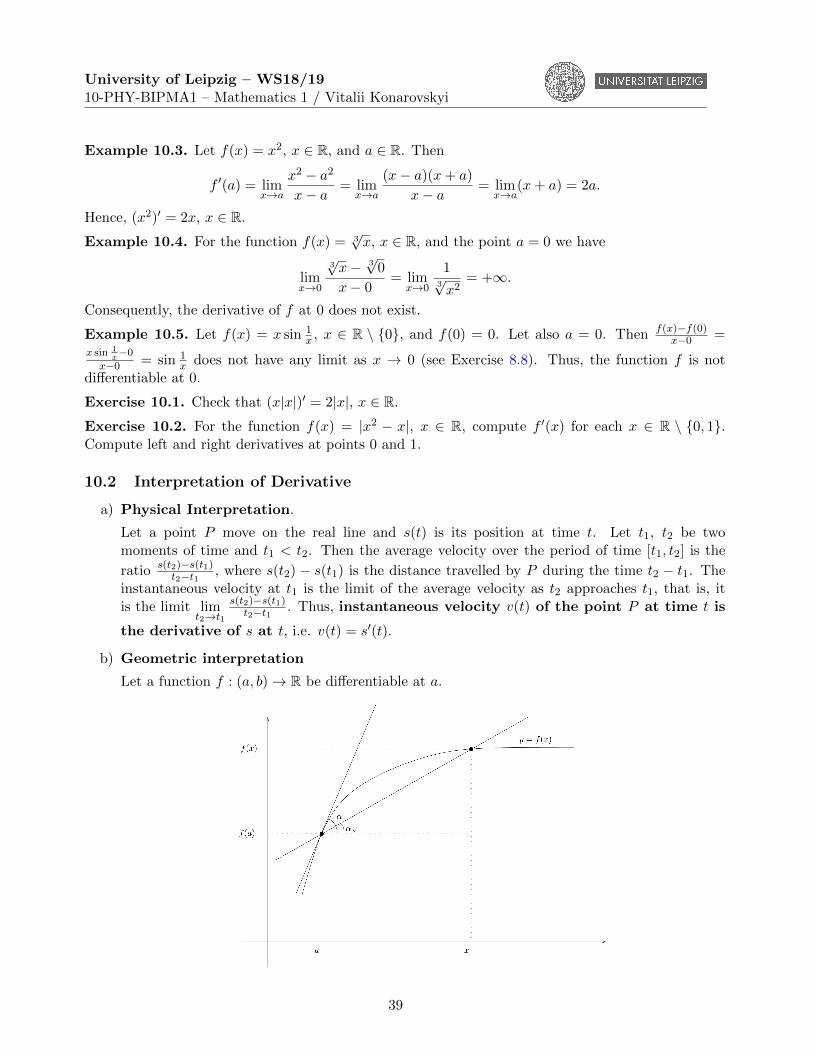
University of Leipzig – WS18/1910-PHY-BIPMA1 – Mathematics 1 / Vitalii Konarovskyi
Example 10.3. Let f(x) = x2, x ∈ R, and a ∈ R. Then
f ′(a) = limx→a
x2 − a2x− a = lim
x→a
(x− a)(x+ a)
x− a = limx→a
(x+ a) = 2a.
Hence, (x2)′ = 2x, x ∈ R.
Example 10.4. For the function f(x) = 3√x, x ∈ R, and the point a = 0 we have
limx→0
3√x− 3√
0
x− 0= lim
x→0
13√x2
= +∞.
Consequently, the derivative of f at 0 does not exist.
Example 10.5. Let f(x) = x sin 1x , x ∈ R \ {0}, and f(0) = 0. Let also a = 0. Then f(x)−f(0)
x−0 =x sin 1
x−0
x−0 = sin 1x does not have any limit as x → 0 (see Exercise 8.8). Thus, the function f is not
differentiable at 0.
Exercise 10.1. Check that (x|x|)′ = 2|x|, x ∈ R.
Exercise 10.2. For the function f(x) = |x2 − x|, x ∈ R, compute f ′(x) for each x ∈ R \ {0, 1}.Compute left and right derivatives at points 0 and 1.
10.2 Interpretation of Derivative
a) Physical Interpretation.
Let a point P move on the real line and s(t) is its position at time t. Let t1, t2 be twomoments of time and t1 < t2. Then the average velocity over the period of time [t1, t2] is the
ratio s(t2)−s(t1)t2−t1 , where s(t2) − s(t1) is the distance travelled by P during the time t2 − t1. The
instantaneous velocity at t1 is the limit of the average velocity as t2 approaches t1, that is, itis the limit lim
t2→t1s(t2)−s(t1)t2−t1 . Thus, instantaneous velocity v(t) of the point P at time t is
the derivative of s at t, i.e. v(t) = s′(t).
b) Geometric interpretation
Let a function f : (a, b)→ R be differentiable at a.
39
University of Leipzig – WS18/1910-PHY-BIPMA1 – Mathematics 1 / Vitalii Konarovskyi
The slope of the secant line through (a, f(a)) and (x, f(x)) is
tanαx =f(x)− f(a)
x− a .
If x approaches a, the secant line through (a, f(a)) and (x, f(x)) approaches the tangent linethrough (a, f(a)). Hence, the derivative f ′(a) is the slope of the tangent line throughthe point (a, f(a)), that is,
tanα = limx→a
f(x)− f(a)
x− a = f ′(a).
So, the linear function whose graph is the tangent line through (a, f(a)) can be given by theequation
f ′(a) = tanα =y − f(a)
x− a , x ∈ R,
that is,y = f(a) + f ′(a)(x− a), x ∈ R.
10.3 Properties of Derivatives
Theorem 10.1. If a function f : A→ R is differentiable at a, then there exists a function ϕ : A→ Rsuch that
f(x) = f(a) + f ′(a)(x− a) + ϕ(x)(x− a), x ∈ Aand ϕ(x)→ 0, x→ a.
Proof. We take ϕ(x) := f(x)−f(a)x−a −f ′(a), x ∈ A\{a} and ϕ(a) = 0. Then the statement easily follows
from Definition 10.1.
Exercise 10.3. If there exists L ∈ R such that f(x) = f(a) +L(x−a) +ϕ(x)(x−a), x ∈ A, for somefunction ϕ : A → R satisfying ϕ(x) → 0, x → a, then f is differentiable at a and f ′(a) = L. Provethis statement.
Theorem 10.2. If f is differentiable at a point a, then f is continuous at a.
Proof. Using theorems 10.1 and 8.1, we obtain
limx→a
f(x) = limx→a
(f(a) + f ′(a)(x− a) + ϕ(x)(x− a)
)= f(a).
Exercise 10.4. Let f has a derivative f ′(a) at a point a. Express through f(a) and f ′(a) the followinglimits:a) lim
h→0
f(a−h)−f(a)h ; b) lim
h→0
f(a+2h)−f(a)h ; c) lim
h→0
f(a+h)−f(a−h)h ; d) lim
n→∞n(f(a+ 1
n
)− f(a)
);
e) limn→∞
n(f(n+1n a
)− f(a)
); f) lim
x→1
f(xa)−f(a)x−1 ; g) lim
n→∞
(f(a+ 1
n)f(a)
)n, f(a) 6= 0.
Exercise 10.5. Prove that f is continuous at a point a if f ′−(a) and f ′+(a) exist.
40
University of Leipzig – WS18/1910-PHY-BIPMA1 – Mathematics 1 / Vitalii Konarovskyi
Theorem 10.3 (Differentiation rules). Let functions f, g : A→ R have derivatives f ′(a) and g′(a) ata point a. Then
1) for each c ∈ R the function cf has a derivative at a and (cf)′(a) = cf ′(a);
2) the function f + g has a derivative at a and (f + g)′(a) = f ′(a) + g′(a);
3) the function f · g has a derivative at a and (f · g)′(a) = f ′(a)g(a) + f(a)g′(a);
4) if additionally g(a) 6= 0, then the function fg has a derivative at a and
(fg
)′(a) = f ′(a)g(a)−f(a)g′(a)
g2.
Proof. Proof of 2). By the definition of derivative and Theorem 8.1 b), we have
(f + g)′(a)Def. 10.1
= limx→a
f(x) + g(x)− (f(a) + g(a))
x− a = limx→a
(f(x)− f(a)
x− a +g(x)− g(a)
x− a
)Th. 8.1
= limx→a
f(x)− f(a)
x− a + limx→a
g(x)− g(a)
x− aDef. 10.1
= f ′(a) + g′(a).
Proof of 3). We compute
(f · g)′(a)Def. 10.1
= limx→a
f(x)g(x)− f(a)g(a)
x− a = limx→a
f(x)g(x)− f(a)g(x) + f(a)g(x)− f(a)g(a)
x− a= lim
x→a
(f(x)− f(a)
x− a g(x) + f(a)g(x)− g(a)
x− a
)Th. 8.1
= limx→a
f(x)− f(a)
x− a limx→a
g(x)
+ f(a) limx→a
g(x)− g(a)
x− a(Def. 10.1+Th. 10.2)
= f ′(a)g(a) + f(a)g′(a).
Proof of 4). Since g(a) 6= 0, we have that g(x) 6= 0 in some neighbourhood of the point a, bytheorems 10.2 and 8.2. Thus,
1
x− a
(f(x)
g(x)− f(a)
g(a)
)=f(x)g(a)− f(a)g(a) + f(a)g(a)− f(a)g(x)
g(x)g(a)(x− a)
=1
g(x)g(a)
(f(x)− f(a)
x− a g(a)− f(a)g(x)− g(a)
x− a
).
Thus, the needed equality follows from the latter relation and theorems 10.2 and 8.1.
Theorem 10.4 (Chain rule). Let a function f : A → R have a derivative f ′(a) at a point a ∈ A.Let f(A) ⊂ B and a function g : B → R have a derivative g′(b) at the point b = f(a). Then thecomposition g ◦ f = g(f) has a derivative at the point a and
(g ◦ f)′(a) = (g(f))′(a) = g′(f(a))f ′(a).
Proof. By Theorem 10.1,g(y)− g(b) = g′(b)(y − b) + ϕ(y)(y − b),
for some function ϕ : B → R satisfying ϕ(y) → 0, y → b. Taking y := f(x) and dividing the latterequality by x− a, we obtain
g(f(x))− g(f(a))
x− a = g′(b)f(x)− f(a)
x− a + ϕ(f(x))f(x)− f(a)
x− a
41
University of Leipzig – WS18/1910-PHY-BIPMA1 – Mathematics 1 / Vitalii Konarovskyi
By Theorem 10.2, f(x)→ f(a) = b, x→ a, and, consequently, ϕ(f(x))→ 0, x→ a. So,
(g ◦ f)′(a) = limx→a
g(f(x))− g(f(a))
x− a = g′(b)f ′(a) + 0f ′(a) = g′(f(a))f ′(a).
Example 10.6. Let α ∈ R. Then (xα)′ = αxα−1, x > 0.Indeed, using Remark 10.1 and Theorem 8.8, we obtain for x > 0
(x+ h)α − xαh
= xα−1(1 + h
x
)α − 1hx
→ xα−1 · α, h→ 0.
Exercise 10.6. a) Let n ∈ N. Show that (xn)′ = nxn−1 for all x ∈ R.b) Let m ∈ Z. Show that (xm)′ = mxm−1 for all x ∈ R \ {0}.
Example 10.7. Let a > 0. Then (ax)′ = ax ln a for all x ∈ R. In particular, if a = e, then (ex)′ = ex
for all x ∈ R.Indeed, using Remark 10.1 and Theorem 8.7, we have for x ∈ R
ax+h − axh
= axah − 1
h→ ax · ln a, h→ 0.
Example 10.8. a) (sinx)′ = cosx and (cosx)′ = − sinx for all x ∈ R;b) (tanx)′ = 1
cos2 xfor all x ∈ R \
{π2 + πk : k ∈ Z
};
c) (cotx)′ = − 1sin2 x
for all x ∈ R \ {πk : k ∈ Z}.Let us check the equalities in a). For every x ∈ R we have
sin(x+ h)− sinx
h=
2
hsin
h
2cos
(x+
h
2
)=
sin h2
h2
cos
(x+
h
2
)→ cosx, h→ 0.
Thus, (sinx)′ = cosx, x ∈ R.Similarly,
cos(x+ h)− cosx
h= −2
hsin
h
2sin
(x+
h
2
)= −sin h
2h2
sin
(x+
h
2
)→ − sinx, h→ 0.
Hence, (cosx)′ = − sinx, x ∈ R.In order to compute (tanx)′, we will use Theorem 10.3 4). So, for every x ∈ R such that cosx 6= 0
we have
(tanx)′ =
(sinx
cosx
)′=
(sinx)′ · cosx− sinx · (cosx)′
cos2 x=
cos2 x+ sin2 x
cos2 x=
1
cos2 x.
and for every x ∈ R such that sinx 6= 0
(cotx)′ =(cosx
sinx
)′=
(cosx)′ · sinx− cosx · (sinx)′
sin2 x= −sin2 x+ cos2 x
sin2 x= − 1
sin2 x.
Exercise 10.7. Compute derivatives of the following functions:
a) y = 2x1−x2 ; b) y = 3
√1+x2
1−x2 ; c) y = e−x2 sinx; d) y = sin2 x
sinx2; e) y = ex
(1 + cot x2
).
42
University of Leipzig – WS18/1910-PHY-BIPMA1 – Mathematics 1 / Vitalii Konarovskyi
Exercise 10.8. Let f(x) = x2, x ≤ 1, and f(x) = ax+ b, x > 1. For which a, b ∈ R the function f :a) is continuous on R; b) is differentiable on R? Compute f ′.
Exercise 10.9. Show thata) (sinhx)′ = coshx, x ∈ R; b) (coshx)′ = sinhx, x ∈ R;c) (tanhx)′ = 1
cosh2 x, x ∈ R; d) (cothx)′ = − 1
sinh2 x, x ∈ R \ {0}.
Exercise 10.10. Let f(x) = 1x3e−
1x2 for x 6= 0 and f(0) = 0. Prove that f ′(0) = 0.
43
University of Leipzig – WS18/1910-PHY-BIPMA1 – Mathematics 1 / Vitalii Konarovskyi
11 Lecture 11 – Derivatives of Inverse Functions and some Theo-rems
11.1 Derivative of Inverse Function
Theorem 11.1 (Differentiation of inverse function). Let −∞ ≤ a < b ≤ +∞ and a function f :(a, b)→ R satisfy the following properties
1) f is continuous on (a, b);
2) f strictly increases on (a, b).
Let (c, d) := f((a, b)) = {f(x) : x ∈ (a, b)}, where −∞ ≤ c < d ≤ +∞. Let also g : (c, d) → (a, b) bethe inverse function to f .
If there exists a derivative f ′(x0) 6= 0 at a point x0 ∈ (a, b), then the function g has a derivativeg′(y0) at the point y0 = f(x0). Moreover,
g′(y0) =1
f ′(x0)=
1
f ′(g(y0)).
Remark 11.1. If a function f : (a, b)→ R is continuous and strictly increasing, then, by Theorem 8.5,the range f((a, b)) of f is an interval and there exists the inverse function g to f which is also continuousand strictly increasing.
Proof of Theorem 11.1. Since the function g is strictly increasing (see Remark 11.1), we have thatg(y) 6= g(y0) for y 6= y0. Using the definition of inverse function and Theorem 10.1, we obtain
y − y0 = f(g(y))− f(g(y0)) = f ′(g(y0))(g(y)− g(y0)) + ϕ(g(y))(g(y)− g(y0)),
where ϕ(g(y)) → 0 as g(y) → g(y0). Since g is continuous on (c, d), one has g(y) → g(y0), y → y0.Thus, ϕ(g(y))→ 0, y → y0. Consequently,
g(y)− g(y0)
y − y0=
g(y)− g(y0)
f ′(g(y0))(g(y)− g(y0)) + ϕ(g(y))(g(y)− g(y0))
=1
f ′(g(y0)) + ϕ(g(y))→ 1
f ′(g(y0)), y → y0.
Remark 11.2. Let us assume that, in Theorem 11.1, the function f has a derivative f ′(x) 6= 0 ateach point x ∈ (a, b). Then for each y ∈ (c, d) there exists the derivative g′(y) and one can get arelationship between f ′ and g′ using the equalities g(f(x)) = x, x ∈ (a, b), and f(g(y)) = y, y ∈ (c, d).Indeed, by the chain rule (see Theorem 10.4), g′(f(x))f ′(x) = 1, x ∈ (a, b), and f ′(g(y))g′(y) = 1,y ∈ (c, d).
Example 11.1. Let α > 0, α 6= 1. Then (logα x)′ = 1x lnα for all x > 0. In particular, (lnx)′ = 1
x forall x > 0.
We will consider the case α > 1. To compute the derivative (logα x)′, we are going to use The-orem 11.1. So, we set f(x) := αx, x ∈ (a, b) := R and (c, d) := (0,+∞). Then f is continuousand strictly increasing on R. Moreover, f ′(x) = αx lnα 6= 0, x ∈ R, by Example 10.7. So, applying
44
University of Leipzig – WS18/1910-PHY-BIPMA1 – Mathematics 1 / Vitalii Konarovskyi
Theorem 11.1, to the function g(y) = logα y, y ∈ (c, d) = (0,+∞), which is inverse to f , we get fory0 ∈ (0,+∞)
g′(y0) = (logα y0)′ =
1
f ′(x0)=
1
αx0 lnα=
1
y0 lnα,
where y0 = f(x0) = αx0 .
Exercise 11.1. Show that (logα x)′ = 1x lnα , x > 0, for 0 < α < 1.
Example 11.2. For all x ∈ R (arctanx)′ = 11+x2
.
Again we are going to use Theorem 11.1. We set f(x) := tanx, x ∈ (a, b) :=(−π
2 ,π2
)and
(c, d) := R. By Example 8.5, f is continuous on(−π
2 ,π2
). Moreover, it is strictly increasing and
f ′(x) = 1cos2 x
6= 0, x ∈(−π
2 ,π2
). Thus, applying Theorem 11.1 to g(y) = arctan y, y ∈ R, we have for
each y0 ∈ Rg′(y0) = (arctan y0)
′ =1
f ′(x0)= cos2 x0 =
1
1 + tan2 x0=
1
1 + y20,
where y0 = f(x0) = tanx0.
Exercise 11.2. For all x ∈ R (arccotx)′ = − 11+x2
.
Example 11.3. For each x ∈ (−1, 1) (arcsinx)′ = 1√1−x2 .
We set f(x) := sinx, x ∈ (a, b) :=(−π
2 ,π2
)and (c, d) := (−1, 1). By Example 8.5, f is continuous on(
−π2 ,
π2
). Moreover, f is strictly increasing and f ′(x) = cosx 6= 0 for all x ∈
(−π
2 ,π2
), by Example 10.8.
Thus, applying Theorem 11.1 to the function g(x) = arcsin y, y ∈ (−1, 1), we obtain for y0 ∈ (−1, 1)
g′(y0) = (arcsin y0)′ =
1
f ′(x0)=
1
cosx0=
1√1− sin2 x0
=1√
1− y20,
where y0 = f(x0) = sinx0.
Exercise 11.3. Show that for each x ∈ (−1, 1) (arccosx)′ = − 1√1−x2 .
Example 11.4. Compute the derivative of the function f(x) = xx, x > 0.Solution. For x > 0 we have (xx)′ =
(elnx
x)′=(ex lnx
)′= ex lnx(x lnx)′ = xx ((x)′ lnx+ x(lnx)′) =
xx(lnx+ x 1
x
)= xx (lnx+ 1).
11.2 Some Theorems
Theorem 11.2 (Fermat theorem). Let f : (a, b) → R, x0 ∈ (a, b) and f(x0) = maxx∈(a,b)
f(x) or
f(x0) = minx∈(a,b)
f(x). If f has a derivative at the point x0, then f ′(x0) = 0.
Proof. We assume that f(x0) = maxx∈(a,b)
f(x). Then for each x ∈ (a, b) f(x) ≤ f(x0). Thus, by
Remark 10.2, we have
f ′(x0) = f ′−(x0) = limx→x0−
f(x)− f(x0)
x− x0≥ 0
and, similarly,
f ′(x0) = f ′+(x0) = limx→x0+
f(x)− f(x0)
x− x0≤ 0.
This implies that f ′(x0) = 0.The case f(x0) = min
x∈(a,b)f(x) is similar.
45
University of Leipzig – WS18/1910-PHY-BIPMA1 – Mathematics 1 / Vitalii Konarovskyi
Remark 11.3. In the Fermat theorem, the assumption a < x0 < b is essential. Indeed, the statementis not valid for the function f(x) = x, x ∈ [0, 1]. In that case, x0 = 1, but f ′(x0) = 1.
Theorem 11.3 (Rolle’s theorem). Let f : [a, b]→ R satisfies the following properties
1) f is continuous on [a, b];
2) for each x ∈ (a, b) the derivative f ′(x) exists;
3) f(a) = f(b).
Then there exists c ∈ (a, b) such that f ′(c) = 0.
Proof. If for every x ∈ [a, b] f(x) = f(a), then f is a constant function. Consequently, f ′(c) = 0 forall c ∈ (a, b).
We now assume that∃x ∈ [a, b] such that f(x) 6= f(a). (9)
According to the assumption 1) and the 2nd Weierstrass theorem (see Theorem 9.2), there existx∗, x
∗ ∈ [a, b] such that f(x∗) = minx∈[a,b]
f(x) and f(x∗) = maxx∈[a,b]
f(x). Using assumptions (9) and 3),
we have that f(x∗) 6= f(a) or f(x∗) 6= f(a). We consider the case f(x∗) 6= f(a). In this case, wehave x∗ 6= a and x∗ 6= b, which implies that x∗ ∈ (a, b). Hence, the function f and the point x0 = x∗
satisfy all assumptions of the Fermat theorem (see Theorem 11.2). Consequently, f ′(x∗) = 0. We takec := x∗.
The case f(x∗) 6= f(a) can be considered similarly.
Exercise 11.4. Let a function f ∈ C([a, b]) have the derivative f ′(x) 6= 0 for all x ∈ (a, b). Thenf(a) 6= f(b).
Theorem 11.4 (Lagrange (mean value) theorem). We assume that a function f : [a, b]→ R satisfiesthe following properties
1) f is continuous on [a, b];
2) f is differentiable on (a, b), that is, f has a derivative f ′(x) for all x ∈ (a, b).
Then there exists c ∈ (a, b) such that f(b)− f(a) = f ′(c)(b− a).
Proof. We take
g(x) := f(x)− f(a)− f(b)− f(a)
b− a (x− a), x ∈ [a, b],
and note that g satisfies the assumptions of Rolle’s theorem (see Theorem 11.3). Moreover,
g′(x) = f ′(x)− f(b)− f(a)
b− a , x ∈ (a, b).
By Rolle’s theorem, there exists c ∈ (a, b) such that g′(c) = 0. It implies that f ′(c) − f(b)−f(a)b−a = 0.
Consequently, f(b)− f(a) = f ′(c)(b− a).
Exercise 11.5. Let a function f : (a, b) → R be differentiable on (a, b) and there exists L ∈ R suchthat |f ′(x)| ≤ L for all x ∈ (a, b). Show that f is uniformly continuous on (a, b).
46
University of Leipzig – WS18/1910-PHY-BIPMA1 – Mathematics 1 / Vitalii Konarovskyi
Theorem 11.5 (Cauchy theorem). Let functions f, g : [a, b]→ R satisfy the following conditions
1) f, g are continuous on [a, b];
2) f, g are differentiable on (a, b);
3) for every x ∈ (a, b) g′(x) 6= 0.
Then there exists c ∈ (a, b) such that f(b)−f(a)g(b)−g(a) = f ′(c)
g′(c) .
Proof. We first note that g(a) 6= g(b). Otherwise, if g(a) = g(b), then there exists c ∈ (a, b) such thatg′(c) = 0, by Rolle’s theorem. But this contradicts assumption 3).
So, we can set
h(x) := f(x)− f(a)− f(b)− f(a)
g(b)− g(a)(g(x)− g(a)), x ∈ [a, b].
Then the function h satisfies the assumptions of Rolle’s theorem. Consequently, there exists c ∈ (a, b)
such that h′(c) = 0. Thus, f ′(c)− f(b)−f(a)g(b)−g(a) g
′(c) = 0.
47

University of Leipzig – WS18/1910-PHY-BIPMA1 – Mathematics 1 / Vitalii Konarovskyi
12 Lecture 12 – Application of Derivatives
12.1 Applications of Lagrange Theorem
Corollary 12.1. Let a function f : (a, b)→ R have the derivative f ′ on (a, b) and for each x ∈ (a, b)f ′(x) = 0. Then there exists L ∈ R such that f(x) = L for all x ∈ (a, b).
Proof. Let x0 ∈ (a, b) be an arbitrary fixed point and x 6= x0. Applying the Lagrange theorem to theinterval with the ends x0 and x, we obtain
f(x)− f(x0) = f ′(c)(x− x0) = 0.
Thus, we can set L := f(x0).
Corollary 12.2. Let functions f, g : (a, b) → R have the derivatives f ′, g′ on (a, b) and for eachx ∈ (a, b) f ′(x) = g′(x). Then there exists L ∈ R such that f(x) = g(x) + L for all x ∈ (a, b).
Proof. Applying Corollary 12.1 to the function f − g, we obtain that there exists a constant L suchthat f(x)− g(x) = L, x ∈ (a, b).
Corollary 12.3. Let a function f : (a, b)→ R have the derivative f ′ on (a, b) and for each x ∈ (a, b)f ′(x) = M , where M is some real number. Then there exists L ∈ R such that f(x) = Mx+ L for allx ∈ (a, b).
Proof. Applying Corollary 12.2 to the functions f and g(x) = Mx, x ∈ (a, b), we obtain the statement.
Exercise 12.1. Let a, b be a fixed numbers. Identify all functions f : R→ R such that f ′(x) = ax+b,x ∈ R.
Exercise 12.2. Identify all functions f : R→ R such that f ′(x) = f(x), x ∈ R.(Hint: Note that (f(x)e−x)′ = (f ′(x)− f(x))e−x, x ∈ R)
Exercise 12.3. Let functions f, g : (a, b)→ (0,+∞) be differentiable on (a, b) and for every x ∈ (a, b)f ′(x)f(x) = g′(x)
g(x) . Prove that there exists L > 0 such that f(x) = Lg(x) for all x ∈ (a, b).(Hint: Consider the functions ln f and ln g)
12.2 Proofs of Inequalities
In this section, we are going to prove a couple of inequalities which are often used in mathematics.
Example 12.1. We prove that for all x1, x2 ∈ Ra) | sinx1− sinx2| ≤ |x1− x2|; b) | cosx1− cosx2| ≤ |x1− x2|; c) | arctanx1− arctanx2| ≤ |x1− x2|.
The proof of these inequalities are similar. So, we will prove only a). We assume that x1 < x2.Then applying the Lagrange theorem to the function f(x) = sinx, x ∈ [x1, x2], we have that thereexists c ∈ (x1, x2) such that
| sinx2 − sinx1| = | cos c| · |x2 − x1| ≤ |x2 − x1|,
since | cos c| ≤ 1.
Exercise 12.4. Prove b) and c) in Example 12.1.
48
University of Leipzig – WS18/1910-PHY-BIPMA1 – Mathematics 1 / Vitalii Konarovskyi
Exercise 12.5. Prove thata) |√x1 −
√x2| ≤ 1
2 |x1 − x2| for all x1, x2 ∈ [1,+∞);
b) |√u2 + v2 −
√u2 + w2| ≤ |v − w| for all u, v, w ∈ R. (Hint: Consider the function f(t) =
√u2 + t2, t ∈ R)
Example 12.2. We prove thata) ex ≥ 1 + x for all x ∈ R, where ex = 1 + x only if x = 0; b) ex > 1 + x+ x2
2 for all x > 0.We prove a). We first assume that x > 0. Then applying the Lagrange theorem to the function
f(u) = eu, u ∈ [0, x], we obtain that there exists c ∈ (0, x) such that ex − e0 = ec · (x − 0). Sinceec > 1 for c > 0, we obtain ex − 1 > x for all x > 0. Next let x < 0. Then we can apply the Lagrangetheorem to the function f(u) = eu, u ∈ [x, 0]. So, we obtain that there exists c ∈ (x, 0) such thate0 − ex = ec · (0− x). Since ec < 1 for c < 0, we get 1− ex < −x.
In order to prove b), we apply the Cauchy theorem to the functions f(u) = eu, g(u) = 1 + u+ u2
2 ,u ∈ [0, x]. Hence, there exists c ∈ (0, x) such that
ex − e01 + x+ x2
2 − 1=
ec
1 + c,
Using a), we have ex − 1 > x+ x2
2 .
Exercise 12.6. Prove that ex > 1 + x+ x2
2! + x3
3! + . . .+ xn
n! for all x > 0 and n ∈ N.(Hint: Use Example 12.2 and mathematical induction)
Exercise 12.7. Prove that x1+x ≤ ln(1 + x) ≤ x for all x > −1.
Exercise 12.8 (Generalised Bernoulli inequality). For each α > 1, prove that (1 + x)α ≥ 1 + αx forall x > −1. Moreover, (1 + x)α = 1 + αx iff x = 0.
Exercise 12.9. Prove thata) x− x3
3! ≤ sinx ≤ x for all x ≥ 0;
b) 1− x2
2 ≤ cosx ≤ 1 for all x ≥ 0.
12.3 Investigation of Monotonicity of Functions
Theorem 12.1. Let −∞ ≤ a < b ≤ +∞ and a function f : (a, b)→ R be differentiable on (a, b).
(i) The function f increases on (a, b) iff f ′(x) ≥ 0 for all x ∈ (a, b).
(ii) The function f decreases on (a, b) iff f ′(x) ≤ 0 for all x ∈ (a, b).
Proof. We prove (i). Let first f ′(x) ≥ 0 for all x ∈ (a, b). We take x1, x2 ∈ (a, b) and x1 < x2. Thenapplying the Lagrange theorem to the function f on the interval [x1, x2], we have that there existsc ∈ (x1, x2) such that
f(x2)− f(x1) = f ′(c)(x2 − x1) ≥ 0. (10)
Next, let f increases on (a, b). Then for each x0 ∈ (a, b)
f ′(x0) = limx→x0
f(x)− f(x0)
x− x0= lim
x→x0+
f(x)− f(x0)
x− x0≥ 0.
Here we used the definition of derivative, Remark 10.2 and the fact that f(x) ≥ f(x0) for x > x0.In order to prove (ii), apply (i) of the theorem to the function g(x) = −f(x), x ∈ (a, b).
49
University of Leipzig – WS18/1910-PHY-BIPMA1 – Mathematics 1 / Vitalii Konarovskyi
Remark 12.1. a) If f ′(x) > 0 for all x ∈ (a, b), then the function f is strictly increasing.
b) If f ′(x) < 0 for all x ∈ (a, b), then the function f is strictly decreasing.Indeed, a) immediately follows from (10), where we have the strict inequality.
We note that the inverse statements of Remark 12.1 is not valid. Indeed, the function f(x) = x3,x ∈ R, strictly increases but its derivative f ′(x) = 3x2, x ∈ R, equals 0 at x = 0.
We formulate more general statement about strictly monotone functions.
Theorem 12.2. Let −∞ ≤ a < b ≤ +∞ and a function f : (a, b)→ R be differentiable on (a, b).
(i) The function f strictly increases on (a, b) iff f ′(x) ≥ 0 for all x ∈ (a, b) and there exists nointerval (α, β) ⊂ (a, b) such that f ′(x) = 0 for all x ∈ (α, β).
(ii) The function f strictly decreases on (a, b) iff f ′(x) ≤ 0 for all x ∈ (a, b) and there exists nointerval (α, β) ⊂ (a, b) such that f ′(x) = 0 for all x ∈ (α, β).
Example 12.3. By Theorem 12.2, the function f(x) = x2 + bx + c, x ∈ R, strictly decreases on(−∞,− b
2
]and strictly increases on
[− b
2 ,+∞), since f ′(x) = 2x + b < 0 for x < − b
2 and f ′(x) =
2x+ b > 0 for x > − b2
Example 12.4. By Theorem 12.2, the function f(x) = ex, x ∈ R, is strictly increasing on R, sincef ′(x) = ex > 0, x ∈ R.
Example 12.5. By Theorem 12.2, the function f(x) = x + sinx, x ∈ R, is strictly increasing on R,since f ′(x) = 1 + cosx > 0 for all x ∈ R \ {x : cosx = −1} = R \ {(2k + 1)π : k ∈ Z}.
Example 12.6. The function f(x) = lnxx , x > 0, strictly increases on (0, e] and strictly decreases on
[e,+∞) according to Theorem 12.2. Indeed, its derivative f ′(x) = 1−lnxx2
, x > 0, is strictly positive on(0, e) and strictly negative on (e,+∞).
Example 12.7. The function f(x) = xx, x > 0, is strictly increasing on[1e ,+∞
)and strictly
decreasing on(−∞, 1e
]according to Theorem 12.2. Indeed, its derivative f ′(x) = xx(1 + lnx), x > 0,
is strictly positive on(1e ,+∞
)and strictly negative on
(−∞, 1e
). For the computation of the derivative
see Example 11.4.
Exercise 12.10. Identify intervals on which the following functions are monotone.a) f(x) = x2 − x, x ∈ R; b) f(x) = x
1+x2, x ∈ R; c) f(x) = 1
x3− 1
x , x ∈ R \ {0};d) f(x) = x+
√|1− x2|, x ∈ R.
Exercise 12.11. Identify a ∈ R for which the function f(x) = x+ a sinx, x ∈ R, is increasing on R.
50
University of Leipzig – WS18/1910-PHY-BIPMA1 – Mathematics 1 / Vitalii Konarovskyi
13 Lecture 13 – L’Hospital’s Rule and Taylor’s Theorem
13.1 L’Hospital’s Rule
Theorem 13.1 (L’Hospital’s Rule). Let a ∈ R or a = −∞ and functions f, g : (a, b)→ R satisfy thefollowing properties
1) f, g are differentiable on (a, b);
2) limx→a+
f(x) = limx→a+
g(x) = 0 or limx→a+
|g(x)| = +∞;
3) g′(x) 6= 0 for all x ∈ (a, b);
4) there exists limx→a+
f ′(x)g′(x) =: L ∈ R.
Then there exists limx→a+
f(x)g(x) = L.
Proof. We will only give a proof for the case a ∈ R and limx→a+
f(x) = limx→a+
g(x) = 0. For the general
case see e.g. [1, p.242-244].We first extend the functions f and g to the interval [a, b), setting f(a) = g(a) := 0. According to
assumption 2), f and g are continuous at the point a. Since f, g are differentiable on (a, b), they arecontinuous also at each point of (a, b), by Theorem 10.2. Thus, f, g are continuous on [a, b). Next, wenote that g(x) 6= 0 for all x ∈ (a, b). Indeed, if g(x0) = 0 for some x0 ∈ (a, b), then applying Rolle’stheorem (see Theorem 11.3) to the function g : [a, x0] → R, we obtain that there exists c ∈ (a, x0)such that g′(c) = 0, that is impossible by assumption 3).
Next, to show that limx→a+
f(x)g(x) = L, we are going to use Theorem 7.7. Let ε > 0 be fixed. By
Theorem 7.7 and assumption 4),
∃δ > 0 ∀x ∈ (a, a+ δ) :
∣∣∣∣f ′(x)
g′(x)− L
∣∣∣∣ < ε.
Applying the Cauchy theorem (see Theorem 11.5) to the functions f, g : [a, x] → R, we have for allx ∈ (a, a+ δ) ∣∣∣∣f(x)
g(x)− L
∣∣∣∣ =
∣∣∣∣f(x)− f(a)
g(x)− g(a)− L
∣∣∣∣ =
∣∣∣∣f ′(c)g′(c)− L
∣∣∣∣ < ε,
where c ∈ (a, x) ⊂ (a, a+ δ).
Remark 13.1. A similar statement is true for the left-sided limit as x goes to b.
Example 13.1. Using L’Hospital’s Rule, we compute the following limits:
a) limx→0
sinxx
00= limx→0
(sinx)′
(x)′ = limx→0
cosx1 = 1;
b) limx→0+
x lnx0·∞= lim
x→0+
lnx1x
∞∞= lim
x→0+
(lnx)′
( 1x)′ = lim
x→0+
1x(− 1x2
) = − limx→0+
x = 0;
c) limx→0
(cosx)1x2
1∞= lim
x→0e
1x2
ln cosx.
We compute
limx→0
1x2
ln cosx = limx→0
ln cosxx2
00= limx→0
(ln cosx)′
(x2)′ = limx→0
− sin xcos x2x = −1
2 limx→0
sinxx cosx = −1
2 limx→0
sinxx · limx→0
1cosx = −1
2 .
51
University of Leipzig – WS18/1910-PHY-BIPMA1 – Mathematics 1 / Vitalii Konarovskyi
Thus, by the continuity of the function f(x) = ex, x ∈ R, we have
limx→0
e1x2
ln cosx = elimx→0
1x2
ln cosx= e−
12 = 1√
e.
See [1, p.245-248] for more examples of the application of L’Hospital’s Rule.
Exercise 13.1. Using L’Hospital’s Rule, show that
a) limx→0
1−cosxx2
= 1; b) limx→0
ln(1+x)sinx = 1; c) lim
x→e(lnx)α−(xe )
β
x−e = α−βe , where α, β are some real numbers;
d) limx→1
( 4πarctanx)
α−1lnx = 2α
π , α ∈ R; e) limx→0+
(ln(1+x)
x
) 1x
= e−12 ; f) lim
x→+∞x2x = 0;
g) limx→+∞
lnxxε = 0 for all ε > 0; h) lim
x→+0xε lnx = 0 for all ε > 0; i) lim
x→+0(ln(1 + x))x = 1.
Exercise 13.2. Compute the following limits:a) lim
x→0
ln(1+x)−xx2
; b) limx→0
ex−esin xx−sinx ; c) lim
x→+∞
(x(π2 − arctanx
)); d) lim
x→+∞ln(x+1)−ln(x−1)√x2+1−
√x2−1 ;
e) limx→+∞
(x sin 1
x + 1x
)x; f) lim
x→+∞
(x sin 1
x + 1x2
)x; g) lim
x→0
(1+x)1x−e
x ; h) limx→+∞
xln x
(lnx)x .
13.2 Higher Order Derivatives
We assume that a function f : (a, b)→ R is differentiable on (a, b). We denote its derivative f ′ by g,that is g(x) = f ′(x), x ∈ (a, b).
Definition 13.1. If there exists a derivative g′(x0) of the function g at a point x0, then this derivative
is called the second derivative of f at the point x0 and is denoted by f ′′(x0) or d2fdx2
(x0).
Let the n-th derivative f (n) be defined on (a, b). Then the (n+1)-th derivative of f at x0 ∈ (a, b)
is defined as f (n+1)(x0) = d(f (n))dx (x0), if it exists.
Example 13.2. Let a > 0. Then for each x ∈ R we obtain (ax)′ = ax ln a, (ax)′′ = ax ln2 a,(ax)′′′ = ax ln3 a, ..., (ax)(n) = ax lnn a. In particular, (ex)(n) = ex, x ∈ R.
Exercise 13.3. Let α ∈ R. Show that (xα)n = α(α− 1)(α− 2) . . . (α− n+ 1)xα−n for all x > 0 andn ∈ N.
Example 13.3. Let α ∈ R. Then ((1 + x)α)(n) = α(α − 1)(α − 2) . . . (α − n + 1)(1 + x)α−n for allx > −1 and n ∈ N.
Indeed, ((1 + x)α)′ = α(1 + x)α−1, ((1 + x)α)′′ =(α(1 + x)α−1
)′= α(α− 1)(1 + x)α−2 and so on.
Exercise 13.4. Show that (ln(1 + x))(n) = (−1)n−1(n−1)!(1+x)n for all x > −1 and n ∈ N.
Example 13.4. For each x ∈ R (sinx)(n) = sin(x+ nπ2
)and (cosx)(n) = cos
(x+ nπ2
).
Indeed, (sinx)′ = cosx = sin(x+ π
2
), (sinx)′′ = (cosx)′ = − sinx = sin
(x+ 2π2
), (sinx)′′′ =
(− sinx)′ = − cosx = sin(x+ 3π2
)and so on. The same computation for (cosx)(n).
Exercise 13.5. Compute the n-th derivative of the following functions:a) f(x) = 2x−1, x ∈ R; b) f(x) =
√1 + x, x > −1; c) f(x) = arctanx, x ∈ R.
Theorem 13.2. Let functions f, g : (a, b) → R have n-th derivatives on (a, b). Then the followingequalities are true.
52
University of Leipzig – WS18/1910-PHY-BIPMA1 – Mathematics 1 / Vitalii Konarovskyi
1) for all k ∈ {1, . . . , n} (f (n−k))(k) = (f (k))(n−k) = f (n), where f (0) = f ;
2) for all c ∈ R (cf)(n) = cf (n);
3) (f + g)(n) = f (n) + g(n).
Theorem 13.3 (Leibniz Formula). For a number n ∈ N let g, f : (a, b)→ R have n-th derivatives on(a, b). Then f · g has the n-th derivative on (a, b) and
(f · g)(n) =
n∑k=0
Cknf(k)g(n−k),
where Ckn = n!k!(n−k)! .
Exercise 13.6. Compute the following derivatives:a) (x2ex)(n), x ∈ R; b) (x3 sinx)(n), x ∈ R; c) (xn lnx)(n), x > 0.
13.3 Taylor’s Formula
13.3.1 Taylor’s Formula for a Polynomial
Let n ∈ N and {a0, a1, a2, . . . , an} ⊂ R. For any point x0 ∈ R a polynomial
P (x) = a0 + a1x+ a2x2 + . . .+ anx
n, x ∈ R,
can be written in the form
P (x) = b0 + b1(x− x0) + b2(x− x0)2 + . . .+ bn(x− x0)n, x ∈ R, (11)
where {b0, b1, b2, . . . , bn} are some real numbers, which can be computed by the following way. Insertingx = x0 into (11), we obtain b0 = P (x0). Next we compute P ′. So,
P ′(x) = b1 + 2b2(x− x0) + 3b3(x− x0)2 + . . .+ nbn(x− x0)n−1, x ∈ R. (12)
Inserting x = x0 into (12), we get b1 = P ′(x0). Next, we compute the second derivative of P
P ′′(x) = 2b2 + 3 · 2 · b3(x− x0) + . . .+ n(n− 1)bn(x− x0)n−2, x ∈ R. (13)
Inserting x = x0 into (13), we obtain b2 = P ′′(x0)2 . Similarly, we obtain
bk =P (k)(x0)
k!, k ≥ 0.
Thus, for each x ∈ R
P (x) = P (x0) +P ′(x0)
1!(x− x0) +
P ′′(x0)
2!(x− x0)2 + . . .+
P (n)(x0)
n!(x− x0)n. (14)
We see that any polynomial can be completely defined only by its value and values of its derivativesat a point x0. Formula (14) does not hold if P is not a polynomial, but it turns out that values of afunction are close to the right hand side of (14) if x is close to x0.
53
University of Leipzig – WS18/1910-PHY-BIPMA1 – Mathematics 1 / Vitalii Konarovskyi
13.3.2 Taylor’s Formula with Peano Remainder Term
Let f, g : A → R be some functions and x0 be a limit point of A. If f(x)g(x) → 0, x → x0, then we will
write f(x) = o(g(x)), x→ 0, or f = o(g), x→ x0.
Exercise 13.7. Show thata) x = o(1), x→ 0; b) x3 = o(2x), x→ +∞; c) lnx = o(
√x), x→ +∞; d) x− sinx = o(x), x→ 0.
Theorem 13.4. Let n ∈ N and let a function f : (a, b) → R and a point x0 ∈ (a, b) satisfy thefollowing conditions:
1) there exists f (n−1)(x) for all x ∈ (a, b);
2) there exists f (n)(x0).
Then
f(x) =
n∑k=0
f (k)(x0)
k!(x− x0)k + o((x− x0)n), x→ x0. (15)
The term o((x− x0)n) is called the Peano remainder term.
Proof. We recall that 0! = 1 and set
Rn(x) := f(x)−n∑k=0
f (k)(x0)
k!(x− x0)k, x ∈ (a, b).
According to assumptions 1) and 2), there exists R(n−1)(x) for all x ∈ (a, b) and R(n)(x0). Moreoverit is easy to see that
Rn(x0) = R′n(x0) = R′′n(x0) = . . . = R(n)n (x0) = 0.
Assuming x > x0 and applying the Lagrange theorem (see Theorem 11.4), we have∣∣∣∣ Rn(x)
(x− x0)n∣∣∣∣ =
∣∣∣∣Rn(x)−Rn(x0)
(x− x0)n∣∣∣∣ =
∣∣∣∣R′n(c1)(x− x0)(x− x0)n
∣∣∣∣ =
∣∣∣∣R′n(c1)−R′n(x0)
(x− x0)n−1∣∣∣∣
=
∣∣∣∣R′′n(c2)(c1 − x0)(x− x0)n−1
∣∣∣∣ ≤ ∣∣∣∣ R′′n(c2)
(x− x0)n−2∣∣∣∣ =
∣∣∣∣R′′n(c2)−R′′n(x0)
(x− x0)n−2∣∣∣∣ =
∣∣∣∣R′′′n (c3)(c2 − x0)(x− x0)n−2
∣∣∣∣ ≤ . . .≤∣∣∣∣∣R(n−1)
n (cn−1)−R(n−1)n (x0)
x− x0
∣∣∣∣∣→ ∣∣∣R(n)n (x0)
∣∣∣ = 0, x→ x0+,
where x0 < cn−1 < cn−2 < . . . < c2 < c1 < x. Moreover cn−1 → x0 as x→ x0+.
One can similarly obtain that∣∣∣ Rn(x)(x−x0)n
∣∣∣→ 0, x→ x0−. Consequently,
Rn(x) = o((x− x0)n), x→ x0,
by Theorem 7.8.
Example 13.5. For every n ∈ N
ex = 1 + x+x2
2!+ . . .+
xn
n!+ o(xn), x→ 0.
The formula follows from Theorem 13.4 applying to f(x) = ex, x ∈ R, and the fact that f (k)(0) =e0 = 1 (see Example 13.2).
54
University of Leipzig – WS18/1910-PHY-BIPMA1 – Mathematics 1 / Vitalii Konarovskyi
Example 13.6. For all n ∈ N
ln(1 + x) = x− x2
2+x3
3− . . .+ (−1)n−1
xn
n+ o(xn), x→ 0.
The formula follows from Theorem 13.4 applying to f(x) = ln(1 + x), x > −1, and the fact that
f (k)(0) = (−1)k−1(k−1)!(1+0)k
= (−1)k−1(k − 1)! (see Example 13.4).
Example 13.7. For each α ∈ R and n ∈ N
(1 + x)α = 1 + αx+α(α− 1)x2
2!+ . . .+
α(α− 1) . . . (α− n+ 1)xn
n!+ o(xn), x→ 0.
The formula follows from Theorem 13.4 applying to f(x) = (1 + x)α, x > −1, and the fact thatf (k)(0) = α(α−1)(α−2) . . . (α−k+1)(1+0)α−k = α(α−1)(α−2) . . . (α−k+1) (see Example 13.3).
Exercise 13.8. Show that for every n ∈ N ∪ {0}
sinx = x− x3
3!+x5
5!− . . .+ (−1)n
x2n+1
(2n+ 1)!+ o(x2n+2), x→ 0,
cosx = 1− x2
2!+x4
4!− . . .+ (−1)n
x2n
(2n)!+ o(x2n+1), x→ 0.
Exercise 13.9. Show that for every n ∈ N ∪ {0}
sinhx =ex − e−x
2= x+
x3
3!+x5
5!+ . . .+
x2n+1
(2n+ 1)!+ o(x2n+2), x→ 0,
coshx =ex + e−x
2= 1 +
x2
2!+x4
4!+ . . .+
x2n
(2n)!+ o(x2n+1), x→ 0.
Exercise 13.10. Use Taylor’s formula to compute the limits:
a) limx→0
ex−1−xx2
; b) limx→0
x−sinxex−1−x−x2
2
; c) limx→0
ln(1+x+x2)+ln(1−x−x2)x sinx ; d) lim
x→0
cos(xex)−cos(xe−x)x3
.
55
University of Leipzig – WS18/1910-PHY-BIPMA1 – Mathematics 1 / Vitalii Konarovskyi
14 Lecture 14 – Local Extrema of Function
14.1 Taylor’s Formula with Lagrangian Remainder Term
Theorem 14.1. Let n ∈ N ∪ {0} and f : (a, b) → R. We assume that there exists f (n+1)(x) for allx ∈ (a, b). Then for each x, x0 ∈ (a, b) there exists a point ξ between x and x0 such that
f(x) =
n∑k=0
f (k)(x0)
k!(x− x0)k +
f (n+1)(ξ)
(n+ 1)!(x− x0)n+1. (16)
The term f (n+1)(ξ)(n+1)! (x− x0)n+1 is called the Lagrangian remainder term.
Proof. If x = x0, then formula (16) holds. We assume that x0 < x and consider a new function
g(z) := f(x)−n∑k=0
f (k)(z)
k!(x− z)k − L
(n+ 1)!(x− z)n+1, z ∈ [x0, x],
where the number L is chosen such that g(x0) = 0. We note that the function g is continuous on[x0, x] and has a derivative
g′(z) = −f(n+1)(z)
n!(x− z)n +
L
n!(x− z)n
Moreover, g(x) = 0. By Rolle’s theorem (see Theorem 11.3), there exists ξ ∈ (x0, x) such thatg′(ξ) = 0, that is,
g′(ξ) = −f(n+1)(ξ)
n!(x− ξ)n +
L
n!(x− ξ)n = 0.
Consequently, we have L = f (n+1)(ξ).The case x < x0 is similar.
Remark 14.1. Formula (16) is a generalisation of the Lagrange theorem, which can be obtainedtaking n = 0.
Example 14.1. Let f(x) = ex, x ∈ R, and x0 = 0. Then for all n ∈ N and x ∈ R there exists ξbetween 0 and x such that
ex = 1 + x+x2
2!+ . . .+
xn
n!+
eξ
(n+ 1)!xn+1. (17)
This formula follows from Theorem 14.1 and Example 13.2, since f (k)(0) = e0 = 1.
Remark 14.2. Formula (17) allows to obtain an approximate value of ex, computing the value of the
polynomial 1 + x+ x2
2! + . . .+ xn
n! . Moreover, the error is equal eξ
(n+1)!xn+1. For instance, for x ∈ [0, 3]
and n = 12 we have ∣∣∣∣ eξ
(n+ 1)!xn+1
∣∣∣∣ < e3313
13!<
1
1000.
56
University of Leipzig – WS18/1910-PHY-BIPMA1 – Mathematics 1 / Vitalii Konarovskyi
14.2 Local Extrema of Function
Let f : (a, b)→ R be a given function.
Definition 14.1. • A point x0 is called a point of local maximum (local minimum) of f ,if there exists δ > 0 such that B(x0, δ) = (x0 − δ, x0 + δ) ⊂ (a, b) and f(x) ≤ f(x0) (resp.f(x) ≥ f(x0)) for all x ∈ B(x0, δ).
If x0 is a point of local minimum or local maximum of f , then it is called a point of localextrema of f .
• A point x0 is called a point of strict local maximum (strict local minimum) of f , ifthere exists δ > 0 such that B(x0, δ) ⊂ (a, b) and f(x) < f(x0) (resp. f(x) > f(x0)) for allx ∈ B(x0, δ) \ {x0}.If x0 is a point of strict local minimum or strict local maximum of f , then it is called a pointof strict local extrema of f .
Example 14.2. For the function f(x) = x2, x ∈ R, the point x0 = 0 is a point of strict local minimumof f and f takes the smallest value at this point.
Example 14.3. For the function f(x) = x, x ∈ [0, 1], the points x∗ = 0 and x∗ = 1 are points atwhich the function takes the smallest and the largest values, respectively. But they are not points oflocal extrema.
Theorem 14.2. If x0 is a point of local extrema of f and f has a derivative at x0, then f ′(x0) = 0.
Proof. Let x0 be a point of local maximum. Then by Definition 14.1, there exists δ > 0 such thatB(x0, δ) ⊂ (a, b) and f(x) ≤ f(x0) for all x ∈ B(x0, δ). In particular, f(x0) = max
x∈B(x0,δ)f(x). Applying
the Fermat theorem (see Theorem 11.2) to the function f defined on (x0 − δ, x0 + δ), we obtainf ′(x0) = 0.
Remark 14.3. Theorem 14.2 gives only a necessary condition of local extrema. If f ′(x0) = 0 at somepoint x0 ∈ (a, b), then it does not imply that x0 is a point of local extrema. For instance, for thefunction f(x) = x3, x ∈ R, the point x0 = 0 is not a point of a local extrema while f ′(0) = 0.
Remark 14.4. A point at which derivative does not exist can also be a point of local extrema. Forexample, for the function f(x) = |x|, x ∈ R, the point x0 = 0 is a point of local minimum but thederivative at x0 = 0 does not exist (see Example 10.2).
Definition 14.2. A point x0 ∈ (a, b) is said to be a critical point or stationary point of f , iff ′(x0) = 0.
Remark 14.5. Point of local extrema of f belong to the set of all critical points of f and pointswhere the derivative of f does not exist.
Theorem 14.3. Let x0 be a critical point of f and the function f be differentiable on some neigh-bourhood of the point x0.
a) If for some δ > 0 f ′(x) > 0 for all x ∈ (x0 − δ, x0) and f ′(x) < 0 for all x ∈ (x0, x0 + δ), thenx0 is a point of strict local maximum of f .
b) If for some δ > 0 f ′(x) < 0 for all x ∈ (x0 − δ, x0) and f ′(x) > 0 for all x ∈ (x0, x0 + δ), thenx0 is a point of strict local minimum of f .
57
University of Leipzig – WS18/1910-PHY-BIPMA1 – Mathematics 1 / Vitalii Konarovskyi
Proof. We will only prove a). Since f ′(x) > 0 for all x ∈ (x0 − δ, x0), the function f strictly increaseson (x0 − δ, x0], by Remark 12.1. Hence, f(x) < f(x0) for all x ∈ (x0 − δ, x0). Similarly, f(x0) > f(x)for all x ∈ (x0, x0 + δ), since the function f strictly decreases on [x0, x0 + δ) due to f ′(x) < 0,x ∈ (x0, x0 + δ). Thus, x0 is a point of strict local maximum.
Example 14.4. For the function f(x) = x3 − 3x, x ∈ R, the points 1 and −1 are critical points off , since the derivative f(x) = 3x2 − 3, x ∈ R, equals zero at those points. The point −1 is a point ofstrict local maximum because the derivative changes its sign from “+” to “−”, passing through −1.The point 1 is a point of strict local minimum because the derivative changes its sign from “−” to“+”, passing through 1.
Exercise 14.1. Find points of local extrema of the following functions:a) f(x) = x2ex, x ∈ R; b) f(x) = x+ 1
x , x > 0; c) f(x) = xx, x > 0; d) f(x) = |x|e−x2 , x ∈ R.
Theorem 14.4. Let a function f : (a, b)→ R and a point x0 ∈ (a, b) satisfy the following properties:
1) there exists δ > 0 such that f is differentiable on (x0 − δ, x0 + δ);
2) f ′(x0) = 0;
3) there exists f ′′(x0) and f ′′(x0) 6= 0.
If f ′′(x0) < 0, then x0 is a point of strict local maximum. If f ′′(x0) > 0, then x0 is a point of strictlocal minimum.
Proof. We write for the function f and the point x0 the Taylor formula (see Theorem 13.4). So,
f(x) = f(x0) + f ′(x0)(x− x0) +f ′′(x0)
2!(x− x0)2 + o((x− x0)2), x→ x0.
Hence, for x 6= x0 we have
f(x)− f(x0) = (x− x0)2(f ′′(x0)
2!+o((x− x0)2)
(x− x0)2)
and, hence, f(x)−f(x0) has the same sign as f ′′(x0) on some neighbourhood of x0, since o((x−x0)2)(x−x0)2 → 0,
x→ x0.
Example 14.5. For the function f(x) = x2−x, x ∈ R, the point 12 is a point of strict local minimum,
since f ′(12
)= 0 and f ′′
(12
)= 2 < 0.
Theorem 14.5. Let f : (a, b) → R, a point x0 belong to (a, b) and m ∈ N, m ≥ 2. We also assumethat the following conditions hold:
1) there exists δ > 0 such that f (m−1)(x) exists for all x ∈ (x0 − δ, x0 + δ);
2) f ′(x0) = f ′′(x0) = . . . = f (m−1)(x0) = 0;
3) there exists f (m)(x0) and f (m)(x0) 6= 0.
If m is even and f (m)(x0) < 0, then x0 is a point of local maximum.If m is even and f (m)(x0) > 0, then x0 is a point of local minimum.If m is odd, then x0 is not a point of local extrema.
58
University of Leipzig – WS18/1910-PHY-BIPMA1 – Mathematics 1 / Vitalii Konarovskyi
Proof. The proof of Theorem 14.5 is similar to the proof of Theorem 14.4.
Exercise 14.2. Prove Theorem 14.5.
Exercise 14.3. Find points of local extrema of the following functions:
a) f(x) = x4(1− x)3, x ∈ R; b) f(x) = x2
2 − 14 + 9
4(2x2+1), x ∈ R; c) f(x) =
{e−
1x2 , x 6= 0,
0, x = 0,, x ∈ R.
14.3 Convex and Concave Functions
Let −∞ ≤ a < b ≤ +∞.
Definition 14.3. • A function f : (a, b) → R is said to be a convex function on (a, b), if foreach x1, x2 ∈ (a, b) and α ∈ (0, 1)
f(αx1 + (1− α)x2) ≤ αf(x1) + (1− α)f(x2).
• A function f : (a, b)→ R is said to be a concave function on (a, b), if for each x1, x2 ∈ (a, b)and α ∈ (0, 1)
f(αx1 + (1− α)x2) ≥ αf(x1) + (1− α)f(x2).
Definition 14.4. • A function f : (a, b)→ R is said to be a strictly convex function on (a, b),if for each x1, x2 ∈ (a, b), x1 6= x2, and α ∈ (0, 1)
f(αx1 + (1− α)x2) < αf(x1) + (1− α)f(x2).
• A function f : (a, b) → R is said to be a strictly concave function on (a, b), if for eachx1, x2 ∈ (a, b), x1 6= x2, and α ∈ (0, 1)
f(αx1 + (1− α)x2) > αf(x1) + (1− α)f(x2).
Example 14.6. Let M,L ∈ R. The function f(x) = Mx+ L, x ∈ R, is both convex and concave onR. Indeed, for each x1, x2 ∈ R and α ∈ (0, 1) we have
f(αx1+(1−α)x2) = M(αx1+(1−α)x2)+L = α(Mx1+L)+(1−α)(Mx2+L) = αf(x1)+(1−α)f(x2).
Example 14.7. The function f(x) = |x|, x ∈ R, is convex on R. Indeed, for each x1, x2 ∈ (a, b) andα ∈ (0, 1)
f(αx1 + (1− α)x2) = |αx1 + (1− α)x2| ≤ α|x1|+ (1− α)|x2| = αf(x1) + (1− α)f(x2),
by the triangular inequality (see Theorem 2.5).
Example 14.8. The function f(x) = x2, x ∈ R, is strictly convex on R. To prove this, we fixx1, x2 ∈ R, x1 6= x2, α ∈ (0, 1) and use the inequality 2x1x2 < x21 + x22 which trivially follows from(x1 − x2)2 > 0. Thus,
f(αx1 + (1− α)x2) = (αx1 + (1− α)x2)2 = α2x21 + 2α(1− α)x1x2 + (1− α)2x22
< α2x21 + α(1− α)(x21 + x22) + (1− α)2x22 = αx21 + (1− α)x22 = αf(x1) + (1− α)f(x2).
59
University of Leipzig – WS18/1910-PHY-BIPMA1 – Mathematics 1 / Vitalii Konarovskyi
Theorem 14.6. Let a function f : (a, b)→ R has the derivative f ′(x) for all x ∈ (a, b).
(i) The function f is convex (strictly convex) on (a, b), if f ′ increases (strictly increases) on (a, b).
(ii) The function f is concave (strictly concave) on (a, b), if f ′ decreases (strictly decreases) on (a, b).
Combining theorems 14.6, 12.1 and 12.2 we obtain the following statement.
Theorem 14.7. Let a function f : (a, b)→ R have the second derivative f ′′(x) for all x ∈ (a, b).
(i) The function f is convex (concave) on (a, b) iff f ′′(x) ≥ 0 (resp. f ′′(x) ≤ 0) for all x ∈ (a, b).
(ii) The function f is strictly convex (strictly concave) on (a, b) iff f ′′(x) ≥ 0 (resp. f ′′(x) ≤ 0) forall x ∈ (a, b) and there is no interval (α, β) ⊂ (a, b) such that f ′′(x) = 0 for all x ∈ (α, β).
Exercise 14.4. Identify intervals on which the following functions are convex or concave:a) f(x) = ex, x ∈ R; b) f(x) = lnx, x > 0; c) f(x) = sinx, x ∈ R; d) f(x) = arctanx, x ∈ R;e) f(x) = xα, x > 0, α ∈ R.
Theorem 14.8 (Jensen’s inequality). Let f : (a, b)→ R be a convex function. Then for each n ≥ 2,x1, . . . , xn ∈ (a, b) and α1, . . . , αn ∈ [0, 1], α1 + . . .+ αn = 1, the inequality
f(α1x1 + . . .+ αnxn) ≤ α1f(x1) + . . .+ αnf(xn) (18)
holds.
Proof. We are going to use the mathematical induction to prove the theorem. For n = 2 inequality (18)is true due to the convexity of f .
Next, we assume that inequality (18) holds for some n ≥ 2 and each x1, . . . , xn ∈ (a, b) andeach α1, . . . , αn ∈ [0, 1], α1 + . . . + αn = 1, and prove (18) for n + 1 and x1, . . . , xn+1 ∈ (a, b),α1, . . . , αn+1 ∈ [0, 1], α1 + . . . + αn+1 = 1. We remark that there exists k such that αk < 1. So, letαn+1 < 1. Then, by Definition 14.3 and the induction assumption,
f
(n+1∑k=1
αkxk
)= f
(αn+1xn+1 +
n∑k=1
αkxk
)≤ αn+1f(xn+1) + (1− αn+1)f
(n∑k=1
αk1− αn+1
xk
)
≤ αn+1f(xn+1) + (1− αn+1)
n∑k=1
αk1− αn+1
f(xk) =
n+1∑k=1
αkf(xk).
Example 14.9. The function f(x) = − lnx, x > 0, is convex on (0,+∞), since f ′′(x) = 1x2
> 0,x > 0 (see Theorem 14.7 (i)). Applying (18) to f , for each n ≥ 2, x1, . . . , xn ∈ (0,+∞) andα1, . . . , αn ∈ [0, 1], α1 + . . .+ αn = 1, we have
ln
(n∑k=1
αkxk
)≥
n∑k=1
αk lnxk.
This impliesn∏k=1
xαkk ≤n∑k=1
αkxk (19)
60
University of Leipzig – WS18/1910-PHY-BIPMA1 – Mathematics 1 / Vitalii Konarovskyi
for all n ≥ 2, x1, . . . , xn ∈ (0,+∞) and α1, . . . , αn ∈ [0, 1], α1 + . . . + αn = 1. In particular, takingα1 = . . . = αn = 1
n , we get
n
√√√√ n∏k=1
xk ≤1
n
n∑k=1
xk
for all n ≥ 2, x1, . . . , xn ∈ (0,+∞), which is the inequality of arithmetic and geometric means.
Exercise 14.5 (Young’s inequality). Let p > 1, q > 1 and 1p + 1
q = 1. Prove that xy ≤ xp
p + yq
q for allx, y ∈ (0,+∞).
(Hint: Use inequality (19))
61
University of Leipzig – WS18/1910-PHY-BIPMA1 – Mathematics 1 / Vitalii Konarovskyi
15 Lecture 15 – Antiderivative and Indefinite Integral
15.1 Definitions and Elementary Properties
In this section, J denotes one of the following intervals [a, b], [a, b), (a, b], (a, b), (−∞, a], (−∞, a),[b,+∞), (b,+∞) or (−∞,+∞). Moreover, for a function f : [a, b] → R, we set f ′(a) := f ′+(a) andf ′(b) := f ′−(b).
Definition 15.1. A function F : J → R is said to be an antiderivative or a primitive function ofa function f : J → R, if for each x ∈ J there exists F ′(x) and F ′(x) = f(x).
Example 15.1. An antiderivative of the function f(x) = x, x ∈ R, is the function F (x) = 12x
2, x ∈ R,
since(12x
2)′
= x for all x ∈ R.
The function G(x) = 12x
2 + 1 is also an antiderivative of f because(12x
2 + 1)′
= x for all x ∈ R.
Example 15.2. An antiderivative of the function f(x) =
{0, x < 0,
x, x ≥ 0,is the function F (x) =
{0, x < 0,x2
2 , x ≥ 0.
Indeed, for each x < 0, F ′(x) = 0 and for each x > 0 F ′(x) = x. Moreover, F ′−(0) = 0, F ′+(0) = 0and, thus, F ′(0) = 0, by Remark 10.2.
Remark 15.1. We note if f has an antiderivative, then it is not unique. Indeed, if F is an antideriva-tive of f , then for any constant C ∈ R the function F + C is also an andiderivative of f because foreach x ∈ J (F (x) + C)′ = F ′(x) = f(x). Moreover, if F and G are antiderivatives of f , then thereexists a constant C ∈ R such that F = G+ C, by Corollary 12.2.
Definition 15.2. The indefinite integral of a function f : J → R is the expression F (x) + C,x ∈ J , where F is an antiderivative of f and C denotes an arbitrary constant. The indefinite integralof a function f is denoted by
∫f(x)dx, x ∈ J .
Exercise 15.1. Find antiderivatives of the following functions:a) f(x) = |x|, x ∈ R; b) f(x) = max{1, x2}, x ∈ R; c) f(x) = | sinx|, x ∈ R;d) f(x) = sinx+ | sinx|, x ∈ R.
Exercise 15.2. Let a function f : R→ R has an antiderivative F : R→ R. Find f , if for each x ∈ R:a) F (x) = f(x); b) F (x) = 1
2f(x); c) F (x) = f(x) + 1; d) 2xF (x) = f(x).
Theorem 15.1 (Properties of indefinite integral). Indefinite integral satisfies the following properties:
1) ddx
∫f(x)dx = f(x), x ∈ J ;
2)∫f ′(x)dx = f(x) + C, x ∈ J ;
3)∫
(af(x))dx = a∫f(x)dx, x ∈ J , for all a ∈ R, a 6= 0;
4)∫
(f(x) + g(x))dx =∫f(x)dx+
∫g(x)dx, x ∈ J .
From definitions 15.2 and 15.1 we have that F ′(x) = f(x), x ∈ J , provided∫f(x)dx = F (x) + C,
x ∈ J . Using this relationship, we can get the following list of important indefinite integrals.
•∫xαdx = xα+1
α+1 + C, x ∈ (0,+∞), for all α ∈ R \ {−1};∫xndx = xn
n+1 + C, x ∈ R, for all n ∈ N ∪ {0};
62
University of Leipzig – WS18/1910-PHY-BIPMA1 – Mathematics 1 / Vitalii Konarovskyi
•∫
1xdx = ln |x|+ C on each interval (−∞, 0) and (0,+∞);
•∫axdx = ax
ln a + C, x ∈ R for all a > 0, a 6= 1;
•∫exdx = ex + C, x ∈ R;
•∫
cosxdx = sinx+ C, x ∈ R;
•∫
sinxdx = − cosx+ C, x ∈ R;
•∫
dxcos2 x
= tanx+ C on each interval(−π
2 + nπ, π2 + nπ), n ∈ Z;
•∫
dxsin2 x
= − cotx+ C on each interval (nπ, π + nπ), n ∈ Z;
•∫
dx1+x2
= arctanx+ C, x ∈ R;
•∫
dx√1−x2 = arcsinx+ C, x ∈ (−1, 1).
15.2 Computation of Indefinite Integrals
An elementary function is the compositions of rational, exponential, trigonometric functions and theirinverse functions. A function is called elementary integrable if it has an elementary antiderivative.“Most” functions are not elementary integrable. For example, antiderivatives of f1(x) = e−x
2, x ∈ R;
f2(x) = ex
x , x > 0; f3(x) = sinxx , x > 0; f4(x) = sinx2, x ∈ R; f5(x) = cosx2, x ∈ R, cannot be
expressed as elementary functions.In the following subsections, we will consider some approaches which allow to compute antideriva-
tives of some classes of functions.
15.2.1 Substitution rule
Definition 15.3. The differential df(x) of a differentiable function f is defined by df(x) =f ′(x)dx.
According to Definition 15.3, we set∫f(x)dϕ(x) :=
∫f(x)ϕ′(x)dx.
Theorem 15.2. Let a function f : J1 → R be continuous on J1, g : J → J1 be continuouslydifferentiable on J (i.e. g has the continuous derivative on J) and let
∫f(t)dx = F (t) + C, t ∈ J1.
Then∫f(g(x))g′(x)dx =
∫f(g(x))dg(x) = F (g(x)) + C, x ∈ J .
Proof. Indeed, (F (g(x)))′ = F ′(g(x))g′(x) = f(g(x))g′(x), x ∈ J , by the chain rule.
Example 15.3. Compute∫
sin 5xdx, x ∈ R.Solution. According to Theorem 15.2, we have∫
sin 5xdx =1
5
∫sin 5xd(5x) = |5x = t| = 1
5
∫sin tdt = −1
5cos t+ C = −1
5cos 5x+ C, x ∈ R.
Example 15.4. Compute∫
2xex2dx, x ∈ R.
Solution. By Theorem 15.2, we obtain∫2xex
2dx =
∫ex
2dx2 =
∣∣x2 = t∣∣ =
∫etdt = et + C = ex
2+ C, x ∈ R.
63
University of Leipzig – WS18/1910-PHY-BIPMA1 – Mathematics 1 / Vitalii Konarovskyi
Exercise 15.3. Compute the following indefinite integrals:a)∫
sin2 xdx, x ∈ R; b)∫
sin 2x sin 3xdx, x ∈ R; c)∫
sin3 xdx, x ∈ R; d)∫
dxsinx cos2 x
, x ∈(0, π2
);
e)∫x cosx2dx, x ∈ R; f)
∫dx1−x on (−∞, 1) and (1,+∞).
Theorem 15.3. Let a function f : J → R be continuous, ϕ : J0 → J be continuously differentiableon J0 and let ϕ have an inverse function ϕ−1. Let also G be an antiderivative for the functiong(t) = f(ϕ(t))ϕ′(t), t ∈ J0. Then∫
f(x)dx =
∫f(ϕ(t))dϕ(t) =
∫f(ϕ(t))ϕ′(t)dt = G(t) + C = G(ϕ−1(x)) + C, x ∈ J.
Proof. Let F be an antiderivative of f on J . Then according to the chain rule, we have
(F (ϕ(t)))′ = F ′(ϕ(t))ϕ′(t) = f(ϕ(t))ϕ(t) t ∈ J0.
Thus, there exists a constant C such that G(t) = F (ϕ(t)) + C, t ∈ J0, or G(ϕ−1(x)) = F (x) + C,x ∈ J .
Example 15.5. Compute∫ √
1− x2dx, x ∈ [−1, 1].Solution. Using Theorem 15.3, we have∫ √
1− x2dx =
∣∣∣∣ x = sin tdx = d sin t = cos tdt
∣∣∣∣ =
∫cos2 tdt =
∫1 + cos 2t
2dt
=1
2t+
1
4sin 2t+ C =
1
2arcsinx+
1
2x√
1− x2 + C.
Here, we have used that t = arcsinx and sin 2t = 2 sin t cos t = 2 sin t√
1− cos2 t = x√
1− x2, forx = sin t, t ∈
(−π
2 ,π2
).
Exercise 15.4. Compute the following indefinite integrals:
a)∫
dxcosx , x ∈
(−π
2 ,π2
); b)
∫1√x2+1
, x ∈ R; c)∫e1x dxx2
, x > 0; d)∫ (2x+1)dx
3√1+x+x2, x ∈ R;
e)∫ √
1− 3xdx, x < 13 ; f)
∫ √tanx
cos2 xdx, x ∈
(0, π2
); g)
∫dxx lnx , x > 0; h)
∫cos2 x sin3 xdx, x ∈ R;
i)∫
dxx2+x+1
, x ∈ R; j)∫
dx1−x2 on (−∞,−1), (−1, 1) and (1,+∞).
15.2.2 Integration by Parts Formula
Theorem 15.4. Let u, v : J → R be differentiable on J and the function uv′ has an antiderivative onJ . Then the function u′v also has an antiderivative on J and the following equality∫
u′(x)v(x)dx = u(x)v(x)−∫u(x)v′(x)dx, x ∈ J, (20)
holds.
Proof. The function uv is antiderivative of the function u′v + uv′ on J , by Theorem 10.3 3). Thus,∫(u′(x)v(x) + u(x)v′(x))dx = u(x)v(x) + C,
which implies equality (20).
64
University of Leipzig – WS18/1910-PHY-BIPMA1 – Mathematics 1 / Vitalii Konarovskyi
Remark 15.2. According to Definition 15.3, the integration by parts formula (20) can be written asfollows ∫
v(x)du(x) = u(x)v(x)−∫u(x)dv(x), x ∈ J.
Example 15.6. Compute∫x sinxdx, x ∈ R.
Solution. Using Theorem 15.4 and Remark 15.2, we have∫x sinxdx = −
∫xd cosx = −x cosx+
∫cosxdx = −x cosx+ sinx+ C, x ∈ R.
Example 15.7. Compute∫
lnxdx, x > 0.Solution. Using Theorem 15.4 and Remark 15.2, we get∫
lnxdx = x lnx−∫xd lnx = x lnx−
∫dx = x lnx− x+ C, x > 0.
Exercise 15.5. Compute∫ex sinxdx, x ∈ R.
Solution. Applying Theorem 15.4 and Remark 15.2, we obtain∫ex sinxdx =
∫sinxdex = ex sinx−
∫exd sinx = ex sinx−
∫ex cosxdx
= ex sinx−∫
cosxdex = ex sinx− ex cosx+
∫exd cosx
= ex(sinx− cosx)−∫ex sinxdx x ∈ R.
Thus,∫ex sinxdx = 1
2ex(sinx− cosx) + C, x ∈ R.
Exercise 15.6. Compute the following indefinite integrals:a)∫x sinxdx, x ∈ R; b)
∫x2 sinxdx, x ∈ R; c)
∫(lnx)2dx, x > 0; d)
∫ln(x2 + x+ 1)dx, x ∈ R.
Exercise 15.7. Find a mistake in the following reasoning.Using Theorem 15.4 and Remark 15.2, we have∫
dx
x= x · 1
x−∫xd
1
x= 1−
∫x ·(− 1
x2
)dx = 1 +
∫dx
x, x > 0.
Thus, 0 = 1!
65
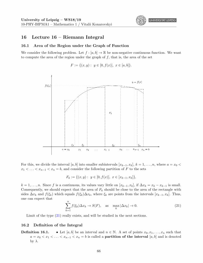
University of Leipzig – WS18/1910-PHY-BIPMA1 – Mathematics 1 / Vitalii Konarovskyi
16 Lecture 16 – Riemann Integral
16.1 Area of the Region under the Graph of Function
We consider the following problem. Let f : [a, b]→ R be non-negative continuous function. We wantto compute the area of the region under the graph of f , that is, the area of the set
F := {(x, y) : y ∈ [0, f(x)], x ∈ [a, b]}.
For this, we divide the interval [a, b] into smaller subintervals [xk−1, xk], k = 1, . . . , n, where a = x0 <x1 < . . . < xn−1 < xn = b, and consider the following partition of F to the sets
Fk := {(x, y) : y ∈ [0, f(x)], x ∈ [xk−1, xk]},
k = 1, . . . , n. Since f is a continuous, its values vary little on [xk−1, xk], if ∆xk = xk − xk−1 is small.Consequently, we should expect that the area of Fk should be close to the area of the rectangle withsides ∆xk and f(ξk) which equals f(ξk)∆xk, where ξk are points from the intervals [xk−1, xk]. Thus,one can expect that
n∑k=1
f(ξk)∆xk → S(F ), as maxk|∆xk| → 0. (21)
Limit of the type (21) really exists, and will be studied in the next sections.
16.2 Definition of the Integral
Definition 16.1. • Let [a, b] be an interval and n ∈ N. A set of points x0, x1, . . . , xn such thata = x0 < x1 < . . . < xn−1 < xn = b is called a partition of the interval [a, b] and is denotedby λ.
66
University of Leipzig – WS18/1910-PHY-BIPMA1 – Mathematics 1 / Vitalii Konarovskyi
• The number |λ| = max{∆xk : 1 ≤ k ≤ n}, where ∆xk = xk − xk−1, is called the mesh of apartition λ.
Let f : [a, b] → R be a function, λ = {x0, x1, . . . , xn} be a partition of the interval [a, b] andξk ∈ [xk−1, xk], k = 1, . . . , n. The sum
n∑k=1
f(ξk)∆xk (22)
is called the Riemann sum.
Definition 16.2. A function f is said to be integrable on [a, b], if there exists a limit J of Riemannsums (22) as |λ| → 0 and this limit does not depend on the choice of partitions λ and points ξk. Moreprecisely, if for all ε > 0 there exists δ > 0 such that for each partition λ = {x0, x1, . . . , xn} with|λ| < δ and points ξk ∈ [xk−1, xk], k = 1, . . . , n,∣∣∣∣∣J −
n∑k=1
f(ξk)∆xk
∣∣∣∣∣ < ε.
The number J is called the Riemann integral of f over [a, b] and is denoted by∫ ba f(x)dx.
Shortly, we will write ∫ b
af(x)dx = lim
|λ|→0
n∑k=1
f(ξk)∆xk. (23)
If f : [a, b]→ R is integrable on [a, b], then we will write f ∈ R([a, b]).
Exercise 16.1. Show that a constant function f(x) = c, x ∈ [a, b], is integrable on [a, b] and compute∫ ba cdx.
Exercise 16.2. Show that the Dirichlet function f(x) = 1, x ∈ Q, and f(x) = 0, x ∈ R \ Q, is notintegrable on any interval [a, b], a < b.
Exercise 16.3. Let f, g : [a, b]→ R be integrable on [a, b]. Show that f + g is also integrable on [a, b].
Theorem 16.1. If a function f : [a, b]→ R is integrable on [a, b], then f is bounded on [a, b].
Exercise 16.4. Prove Theorem 16.1.
Let f : [a, b]→ R be a bounded function on [a, b].
Definition 16.3. • The upper Darboux sum of f with respect to a partition λ is the sum
U(f, λ) =
n∑k=1
Mk∆xk,
where Mk := supx∈[xk−1,xk]
f(x).
• The lower Darboux sum of f with respect to a partition λ is the sum
L(f, λ) =
n∑k=1
mk∆xk,
where mk := infx∈[xk−1,xk]
f(x).
67
University of Leipzig – WS18/1910-PHY-BIPMA1 – Mathematics 1 / Vitalii Konarovskyi
Theorem 16.2 (Integrability criterion). A function f : [a, b] → R is integrable on [a, b] iff for everyε > 0 there exists λ = λ([a, b]) such that
U(f, λ)− L(f, λ) < ε.
Exercise 16.5. Let f ∈ R([a, b]). Show thata) |f | ∈ R([a, b]); b) sin f ∈ R([a, b]); c) f2 ∈ R([a, b]); d) max{0, f} ∈ R([a, b]).
Exercise 16.6. Let f, g ∈ R([a, b]). Show that fg ∈ R([a, b]).
16.3 Classes of Integrable Functions
16.3.1 Integrability of Monotone Functions
Theorem 16.3. Let f : [a, b]→ R be a monotone function on [a, b]. Then f is integrable on [a, b].
Proof. We assume that f is increasing on [a, b] and f(a) < f(b). To prove the theorem, we are going touse the integrability criterion (see Theorem 16.2). For any ε > 0 we take a partition λ of the interval[a, b] such that |λ| < ε
f(b)−f(a) . For such a partition we have
U(f, λ)− L(f, λ) =n∑k=1
(Mk −mk)∆xk =n∑k=1
(f(xk)− f(xk−1))∆xk
≤ |λ|n∑k=1
(f(xk)− f(xk−1)) = |λ|(f(xn)− f(x0)) = |λ|(f(b)− f(a)) < ε.
Exercise 16.7. For any bounded function f : [a, b]→ R we set g(x) = supu∈[a,x]
f(u) and h(x) = infu∈[a,x]
f(u),
x ∈ [a, b]. Show that g, h ∈ R([a, b]).
16.3.2 Integrability of Continuous Functions
Theorem 16.4. Let f : [a, b]→ R be continuous on [a, b]. Then f is integrable on [a, b].
Proof. We will use the integrability criterion again, to prove the theorem. By the Cantor theorem (seeTheorem 9.4), f is uniformly continuous on [a, b]. Thus, for a number ε
b−a > 0 there exists δ > 0 suchthat for each x′, x′′ ∈ [a, b], |x′−x′′| < δ it follows |f(x′)−f(x′′)| < ε
b−a . Next, we choose a partition λof [a, b] with |λ| < δ. Thus, by the 2nd Weierstrass theorem (see Theorem 9.2), for each k = 1, . . . , n
Mk −mk = supx∈[xk−1,xk]
f(x)− infx∈[xk−1,xk]
f(x) = f(x∗)− f(x∗) <ε
b− a,
where x∗ and x∗ are points where f takes its maximum and minimum value on [xk−1, xk], respectively.Consequently,
U(f, λ)− L(f, λ) =n∑k=1
(Mk −mk)∆xk <ε
b− an∑k=1
∆xk = ε.
68
University of Leipzig – WS18/1910-PHY-BIPMA1 – Mathematics 1 / Vitalii Konarovskyi
16.4 Properties of Riemann Integral
Theorem 16.5 (Linearity and addidivity). (i) Let f ∈ R([a, b]) and c ∈ R. Then cf ∈ R([a, b])and ∫ b
acf(x)dx = c
∫ b
af(x)dx.
(ii) Let f, g ∈ R([a, b]). Then f + g ∈ R([a, b]) and∫ b
a(f(x) + g(x))dx =
∫ b
af(x)dx+
∫ b
ag(x)dx.
(iii) Let f ∈ R([a, b]) and c ∈ (a, b). Then f ∈ R([a, c]) and f ∈ R([c, b]). Moreover,∫ b
af(x)dx =
∫ c
af(x)dx+
∫ b
cf(x)dx.
Exercise 16.8. Prove (i) and (ii) of Theorem 16.5.
Exercise 16.9. Let c ∈ (a, b). Show that f ∈ R([a, b]), if f ∈ R([a, c]) and f ∈ R([c, b]).
Theorem 16.6. Let f, g ∈ R([a, b]) and f(x) ≤ g(x), x ∈ [a, b]. Then∫ ba f(x)dx ≤
∫ ba g(x)dx.
Proof. The statement immediately follows from the definition of the integral.
Exercise 16.10. Prove Theorem 16.6.
Corollary 16.1. Let f ∈ R([a, b]) and m := infx∈[a,b]
f(x), M := supx∈[a,b]
f(x). Then
m(b− a) ≤∫ b
af(x)dx ≤M(b− a). (24)
Proof. We first note that m and M exists, since f is bounded (see Theorem 16.1). Inequality (24)follows from the inequality m ≤ f(x) ≤M , x ∈ [a, b], and Theorem 16.6.
Corollary 16.2. Let f ∈ R([a, b]). Then |f | ∈ R([a, b]) and∣∣∣∣∫ b
af(x)dx
∣∣∣∣ ≤ ∫ b
a|f(x)|dx.
Exercise 16.11. Prove Corollary 16.2.
Theorem 16.7 (Mean value theorem for integrals). Let f : [a, b] → R be a continuous function on
[a, b]. Then there exists θ ∈ [a, b] such that∫ ba f(x)dx = f(θ)(b− a).
Proof. By Corollary 16.1,
m ≤ L :=1
b− a
∫ b
af(x)dx ≤M.
Since f is continuous, we can apply the 2nd Weierstrass theorem (see Theorem 9.2) to f . Thus,there exist x∗, x
∗ ∈ [a, b] such that m = f(x∗) and M = f(x∗). Consequently, f(x∗) ≤ L ≤ f(x∗).By the intermediate value theorem (see Theorem 9.3), there exists θ between x∗ and x∗ such thatf(θ) = L.
69
University of Leipzig – WS18/1910-PHY-BIPMA1 – Mathematics 1 / Vitalii Konarovskyi
Exercise 16.12. Let f : [a, b]→ R be a non-negative continuous function on [a, b] such that f(x0) > 0
for some x0 ∈ [a, b]. Show that∫ ba f(x)dx > 0.
Exercise 16.13. Let f ∈ C([a, b]), g ∈ R([a, b]) and g(x) ≥ 0, x ∈ [a, b]. Show that there exists
θ ∈ [a, b] such that∫ ba f(x)g(x)dx = f(θ)
∫ ba g(x)dx.
Exercise 16.14. For functions f, g ∈ R([a, b]) compute the limit
lim|λ|→0
n∑k=1
f(ξk)
∫ xk
xk−1
g(x)dx.
Exercise 16.15. For a function f ∈ R([0, 1]) prove the equality
limn→∞
∫ 1
1n
f(x)dx =
∫ 1
0f(x)dx.
Exercise 16.16 (Cauchy inequality). For f, g ∈ R([a, b]) prove the following inequality(∫ b
af(x)g(x)dx
)2
≤∫ b
af2(x)dx
∫ b
ag2(x)dx.
70
University of Leipzig – WS18/1910-PHY-BIPMA1 – Mathematics 1 / Vitalii Konarovskyi
17 Lecture 17 – Fundamental Theorem of Calculus and Applicationof Riemann Integral
17.1 Fundamental Theorem of Calculus
We set faa f(x)dx := 0 and∫ ab f(x)dx := −
∫ ba f(x)dx for a < b.
Theorem 17.1. Let f : [a, b] → R be integrable on [a, b]. Then the function ϕ(x) :=∫ xa f(u)du,
x ∈ [a, b], is continuous on [a, b].
Proof. For every x′, x′′ ∈ [a, b] we have
|ϕ(x′)− ϕ(x′′)| =∣∣∣∣∣∫ x′
af(x)dx−
∫ x′′
af(x)dx
∣∣∣∣∣ =
∣∣∣∣∣∫ x′′
x′f(x)dx
∣∣∣∣∣ ≤∫ x′′
x′|f(x)|dx ≤ sup
x∈[a,b]|f(x)||x′ − x′′|,
by Theorem 16.5 (iii) and corollaries 16.1, 16.2. Consequently, ϕ is uniformly continuous on [a, b].
Theorem 17.2. Let f : [a, b] → R be continuous on [a, b]. Then the function ϕ(x) :=∫ xa f(u)du,
x ∈ [a, b], is differentiable on [a, b] and ϕ′(x) = f(x), x ∈ [a, b], that is, ϕ is an antiderivative of f on[a, b].
Proof. Let x0 ∈ [a, b] and h 6= 0. By the mean value theorem (see Theorem 16.7), there exists θhbetween x0 and x0 + h such that
ϕ(x0 + h)− ϕ(x0)
h=
1
h
∫ x0+h
x0
f(x)dx = f(θh).
Since θh → x0, h→ 0, and f is continuous, we obtain
limh→0
ϕ(x0 + h)− ϕ(x0)
h= lim
h→0f(θh) = f(x0).
Theorem 17.3 (Fundamental Theorem of Calculus). We assume that f : [a, b] → R satisfies thefollowing properties:
1) f is integrable on [a, b];
2) f has an antiderivative F on [a, b].
Then ∫ b
af(x)dx = F (b)− F (a).
We will also denote F (x)∣∣∣ba
:= F (b)− F (a).
Proof. We first prove the theorem in the case f ∈ C([a, b]). The function ϕ(x) :=∫ xa f(u)du, x ∈ [a, b],
is an antiderivative of f on [a, b], by Theorem 17.2. Thus, using Remark 15.1, there exists C ∈ Rsuch that ϕ(x) = F (x) + C, x ∈ [a, b]. In particular, ϕ(a) = F (a) + C = 0. Thus, C = −F (a).
Consequently,∫ ba f(x)dx = ϕ(b) = F (b) + C = F (b)− F (a).
71
University of Leipzig – WS18/1910-PHY-BIPMA1 – Mathematics 1 / Vitalii Konarovskyi
Next, we give the second proof of the theorem in the general case. Let λ = {x0, x1, . . . , xn} be apartition of [a, b]. We first note that
F (b)−F (a) = (F (x1)−F (x0)) + (F (x2)−F (x1)) + . . .+ (F (xn)−F (xn−1)) =n∑k=1
(F (xk)−F (xk−1)).
We apply the Lagrange theorem (see Theorem 11.4) to the function F on [xk−1, xk] for each k =1, . . . , n. So, there exists ξk ∈ [xk−1, xk], k = 1, . . . , n, such that
F (b)− F (a) =
n∑k=1
(F (xk)− F (xk−1)) =
n∑k=1
F ′(ξk)∆xk =
n∑k=1
f(ξk)∆xk.
Making |λ| → 0, we have
F (b)− F (a) =n∑k=1
f(ξk)∆xk →∫ b
af(x)dx,
since f is integrable on [a, b].
Exercise 17.1. Compute the following integrals:
a)∫ 8−1
3√xdx; b)
∫ π0 sinxdx; c)
∫ √31√3
dx1+x2
; d)∫ 20 |1− x|dx; e)
∫ 1−1
dxx2−2x cosα+1
for α ∈ (0, π).
Example 17.1 (Leibniz’s rule). Let a function f : R → R have an antiderivative on R and beintegrable on each finite interval. Let functions a, bR→ R be differentiable on R. Then
d
dx
∫ b(x)
a(x)f(u)du = f(b(x))b′(x)− f(a(x))a′(x), x ∈ R.
Indeed, let F be an antiderivative of f on R. By the fundamental theorem of calculus,∫ b(x)
a(x)f(u)du = F (b(x))− F (a(x)), x ∈ R. (25)
Moreover, the right hand side of (25) is differentiable and
d
dx(F (b(x))− F (a(x))) = F ′(b(x))b′(x)− F ′(a(x))a′(x) = f(b(x))b′(x)− f(a(x))a′(x), x ∈ R,
by the chain rule.
Exercise 17.2. Compute the following derivatives:
a) ddx
∫ ba sinx2dx; b) d
da
∫ ba sinx2dx; c) d
dx
∫ x20
√1 + t2dt; d) d
dx
∫ x3x2
dt1+t4
.
Exercise 17.3. Compute the following limits:
a) limx→0
∫ x0 cos t2dt
x ; b) limx→+∞
∫ x0 (arctan t)2dt√
x2+1; c) lim
x→+∞
(∫ x0 et
2dt)2∫ x
0 e2t2dt.
72
University of Leipzig – WS18/1910-PHY-BIPMA1 – Mathematics 1 / Vitalii Konarovskyi
17.2 Some Corollaries
Theorem 17.4 (Substitution rule). We assume that f : [a, b] → R is continuous on [a, b] and u :[α, β]→ [a, b] is continuously differentiable on [α, β]. Then the following equality∫ β
αf(u(t))u′(t)dt =
∫ β
αf(u(t))du(t) =
∫ u(β)
u(α)f(x)dx
holds.
Proof. Since the function f is continuous on [u(α), u(β)], it has an antiderivative F on [u(α), u(β)],by Theorem 17.2. Using the fundamental theorem of calculus,∫ u(β)
u(α)f(x)dx = F (u(β))− F (u(α)).
Moreover, the function F (u) is an antiderivative of f(u)u′ on [α, β]. Thus, by the fundamental theoremof calculus, ∫ β
αf(u(t))u′(t)dt = F (u(β))− F (u(α)).
This proves the theorem.
Exercise 17.4. Using the substitution rule, compute the following integrals:
a)∫ √π0 x sinx2dx; b)
∫ 10 e
2x−1dx; c)∫ 1−1
xdx√5−4x ; d)
∫ ln 20
√ex − 1dx; e)
∫ π60
dxcosx .
Theorem 17.5 (Integration by parts). Let u, v : [a, b] → R be continuously differentiable functionson [a, b]. Then ∫ b
au(x)dv(x) = u(x)v(x)
∣∣∣ba−∫ b
av(x)du(x),
i.e. ∫ b
au(x)v′(x)dx = u(b)v(b)− u(a)v(a)−
∫ b
au′(x)v(x)dx.
Proof. Since the function uv is an antiderivative of uv′ + u′v on [a, b],∫ b
a(u(x)v′(x) + u′(x)v(x))dx = u(b)v(b)− u(a)v(a),
by the fundamental theorem of calculus. Using Theorem 16.5 (ii), we obtain the integration by partsformula.
Exercise 17.5. Using the integration by parts formula, compute the following integrals:a)∫ ln 20 xe−xdx; b)
∫ π0 x sinxdx; c)
∫ 2π0 x2 cosxdx; d)
∫ e1e| lnx|dx; e)
∫ 10 arccosxdx.
73
University of Leipzig – WS18/1910-PHY-BIPMA1 – Mathematics 1 / Vitalii Konarovskyi
17.3 Application of the Integral
17.3.1 Area of the Region under the Graph of Function
Theorem 17.6. Let f : [a, b] → R be a continuous function on [a, b] and f(x) ≥ 0, x ∈ [a, b]. Thenthe area of the region
F = {(x, y) : 0 ≤ y ≤ f(x), a ≤ x ≤ b}under the graph of f is equal to
S(F ) =
∫ b
af(x)dx.
Proof. We first note that f is integrable on [a, b] because it is continuous (see Theorem 16.4). Thus,the formula for the area follows from the discussion in Section 16.1 and definition of the integral(see (23)).
Example 17.2. The area of the region under the graph of the function f(x) = x2, x ∈ [0, 1], is equal∫ 1
0x2dx =
x3
3
∣∣∣10
=1
3.
Example 17.3. Compute the area of the region G enclosed by the ellipse x2
a2+ y2
b2= 1, a > 0, b > 0.
In order to compute the area of G, it is enough to compute the area of
F =
{(x, y) : 0 ≤ y ≤ b
√1− x2
a2, 0 ≤ x ≤ a
}.
By Theorem 17.6,
S(G) = 4S(F ) = 4
∫ a
0b
√1− x2
a2dx =
∣∣∣∣ x = a sin tdx = a cos tdt
∣∣∣∣ = 4ab
∫ π2
0cos2 tdt
= 4ab
∫ π2
0
1 + cos 2t
2dt = 2abt
∣∣∣π20
+ ab sin 2t∣∣∣π20
= πab.
Exercise 17.6. Compute the area of regions bounded by the graphs of the following functions:a) 2x = y2 and 2y = x2; b) y = x2 and x+ y = 2; c) y = 2x, y = 2 and x = 0;
d) y = a3
a2+x2and y = 0, where a > 0.
17.3.2 Length of a Curve
Definition 17.1. Let ϕ,ψ : [a, b]→ R be continuous functions on [a, b]. The set of points
Γ := {(x, y) ∈ R2 : x = ϕ(t), y = ψ(t), t ∈ [a, b]} (26)
is called a continuous (plane) curve.
We first give a definition of the length of the continuous curve Γ. Let λ = {t0, t1, . . . , tn} be apartition of [a, b]. We consider the polygonal curve Γλ with vertices (ϕ(tk), ψ(tk)), k = 0, . . . , n. Itslength equals
l(Γλ) =
n∑k=1
√(ϕ(tk)− ϕ(tk−1))2 + (ψ(tk)− ψ(tk−1))2.
74
University of Leipzig – WS18/1910-PHY-BIPMA1 – Mathematics 1 / Vitalii Konarovskyi
Definition 17.2. The curve Γ is said to be a rectifiable curve, if there exists a finite limit
lim|λ|→0
l(Γλ) =: l(Γ),
that is, if there exists a real number l(Γ) such that
∀ε > 0 ∃δ > 0 ∀λ |λ| < δ : |l(Γλ)− l(Γ)| < ε.
The limit l(Γ) is called the length of rectifiable curve Γ.
Theorem 17.7. Let ϕ,ψ : [a, b]→ R be continuously differentiable on [a, b]. Then Γ, defined by (26),is a rectifiable curve and its length equals
l(Γ) =
∫ b
a
√(ϕ′(t))2 + (ψ′(t))2dt.
Proof. Using the Lagrange theorem (see Theorem 11.4), we have
l(Γλ) =n∑k=1
√(ϕ′(ξk))2 + (ψ′(ηk))2∆tk =
n∑k=1
√(ϕ′(ξk))2 + (ψ′(ξk))2∆tk + rλ,
where ξk, ηk ∈ [tk−1, tk], k = 1, . . . , n, and
rλ :=
n∑k=1
√(ϕ′(ξk))2 + (ψ′(ηk))2∆tk −
n∑k=1
√(ϕ′(ξk))2 + (ψ′(ξk))2∆tk.
Since the function f(t) =√
(ϕ′(t))2 + (ψ′(t))2, t ∈ [a, b], is continuous on [a, b], it is integrable on[a, b], by Theorem 16.4. Thus,
lim|λ|→0
n∑k=1
√(ϕ′(ξk))2 + (ψ′(ξk))2∆tk =
∫ b
a
√(ϕ′(t))2 + (ψ′(t))2dt.
Moreover, using the inequality
|√u2 + v2 −
√u2 + w2| ≤ |v − w|, u, v, w ∈ R,
(see Exercise 12.5 b)), we have
|rλ| ≤n∑k=1
|ψ′(ξk)− ψ′(ηk)|∆tk ≤n∑k=1
(Mk −mk)∆tk,
where Mk := supt∈[tk−1,tk]
ψ′(t) and mk := inft∈[tk−1,tk]
ψ′(t), k = 1, . . . , n. Using theorems 16.2 and 16.4, we
obtain
|rλ| ≤n∑k=1
(Mk −mk)∆tk → 0, |λ| → 0.
75
University of Leipzig – WS18/1910-PHY-BIPMA1 – Mathematics 1 / Vitalii Konarovskyi
Remark 17.1. If a curve Γ is given by the graph of a continuously differentiable function f : [a, b]→ R,that is,
Γ = {(x, y) : y = f(x), x ∈ [a, b]},then its length equals
l(Γ) =
∫ b
a
√1 + (f ′(x))2dx.
Example 17.4. We compute the length of the circle x2 + y2 = r2, r > 0, that is, the length of thecurve
Γ ={
(x, y) : x2 + y2 = r2}
= {(x, y) : x = r cos t, y = r sin t, t ∈ [0, 2π)} .By Theorem 17.7,
l(Γ) =
∫ 2π
0
√r2 sin2 t+ r2 cos2 tdt =
∫ 2π
0rdt = 2πr.
Exercise 17.7. Compute the length of continuous curves defined by the following functions:a) y = x
32 , x ∈ [0, 4]; b) y = ex, 0 ≤ x ≤ b; c) x = a(t − sin t), y = a(1 − cos t), t ∈ [0, 2π], where
a > 0.
17.3.3 Volume of Solid of Revolution
Definition 17.3. Let f : [a, b]→ R be a positive continuous function. A solid of revolution G is aset of points in R3 obtained by rotating of the region under the graph of f around the x-axis, that is,
G ={
(x, y, z) : y2 + z2 ≤ f2(x), x ∈ [a, b]}.
Theorem 17.8. Let f : [a, b] → R be a positive continuous function. Then the volume of solid ofrevolution G is equal to
V (G) = π
∫ b
af2(x)dx.
Idea of Proof. We consider a partition λ = {x0, x1, . . . , xn} of the interval [a, b] and split G into smallersets
Gk ={
(x, y, z) : y2 + z2 ≤ f2(x), x ∈ [xk−1, xk]}, k = 1, . . . , n.
Then the volume of Gk is approximately equal the volume of the cylinder{(x, y, z) : y2 + z2 ≤ f2(ξk), x ∈ [xk−1, xk]
},
where ξk ∈ [xk−1, xk]. Thus,
V (G) =
n∑k=1
V (Gk) ≈n∑k=1
πf2(ξk)∆xk.
Passing to the limit as |λ| → 0, we obtain
V (G) = π
∫ b
af2(x)dx.
76
University of Leipzig – WS18/1910-PHY-BIPMA1 – Mathematics 1 / Vitalii Konarovskyi
Example 17.5. The volume of the cone
G = {(x, y, z) : y2 + z2 ≤ x2, x ∈ [0, 1]}.
equals
V (G) = π
∫ 1
0x2dx = π
x3
3
∣∣∣10
=π
3,
since G can be obtained by rotating of the region under the graph of the function f(x) = x, x ∈ [0, 1],around the x-axis.
Exercise 17.8. Compute the volume of the paraboloid of revolution
G = {(x, y, z) : y2 + z2 ≤ x, x ∈ [0, 1]}.
(Hint: G can be obtained by rotating of the region under the graph of the function f(x) =√x, x ∈ [0, 1], around
the x-axis)
77
University of Leipzig – WS18/1910-PHY-BIPMA1 – Mathematics 1 / Vitalii Konarovskyi
18 Lecture 18 – Improper Integrals
18.1 Integrals over Unbounded Intervals
18.1.1 Definition and Elementary Properties
In this section, we assume that a function f : [a,+∞)→ R is integrable on [a, z] for all z > a and set
ϕ(z) :=
∫ z
af(x)dx, z ≥ a.
Definition 18.1. The finite limit
limz→+∞
ϕ(z) = limz→+∞
∫ z
af(x)dx (27)
is called the improper integral of f over [a,+∞) and is denoted by∫ +∞
af(x)dx. (28)
In this case, we will say that improper integral (28) converges. If limit (27) does not exist or isinfinite, then improper integral (28) is said to be divergent.
Remark 18.1. If integral (28) converges, then for each b > a the improper integral∫ +∞
bf(x)dx (29)
also converges. If for some b > a improper integral (29) converges, then improper integral (28) alsoconverges. These both statements follow from the equality∫ z
af(x)dx =
∫ b
af(x)dx+
∫ z
bf(x)dx, a < b ≤ z,
and the definition of the improper integral.
Example 18.1. The improper integral∫ +∞0 e−xdx converges and equals 1. Indeed,∫ +∞
0e−xdx = lim
z→+∞
∫ z
0e−xdx = lim
z→+∞
(−e−x
∣∣∣z0
)= lim
z→+∞(1− e−z) = 1.
Example 18.2. The equality∫ +∞0
dx1+x2
= π2 is true, since∫ +∞
0
dx
1 + x2= lim
z→+∞
∫ z
0
dx
1 + x2= lim
z→+∞
(arctanx
∣∣∣z0
)= lim
z→+∞(arctan z − 0) =
π
2.
Example 18.3. Let p > 0. The improper integral∫ +∞1
dxxp converges for p > 1 and diverges for p ≤ 1.
Indeed, for each z ≥ 1
ϕ(z) =
∫ z
1
dx
xp=
{ln z − ln 1, p = 1,z−p+1
−p+1 − 1−p+1 , p 6= 1.
Thus,
ϕ(z)→{
+∞, p ≤ 1,1p−1 , p > 1,
z → +∞.
78
University of Leipzig – WS18/1910-PHY-BIPMA1 – Mathematics 1 / Vitalii Konarovskyi
Example 18.4. The integral∫ +∞0 cosxdx diverges, since for the function ϕ(z) =
∫ z0 cosxdx = sin z,
z ≥ 0, there is no limit as z → +∞.
Theorem 18.1 (Elementary properties of improper integrals). The following properties of improperintegrals are true.
1) Let integrals∫ +∞a f(x)dx and
∫ +∞a g(x)dx converge. Then the integrals
∫ +∞a cf(x)dx, c ∈ R,∫ +∞
a (f(x) + g(x))dx converge and∫ +∞
acf(x)dx = c
∫ +∞
af(x)dx,∫ +∞
a(f(x) + g(x))dx =
∫ +∞
af(x)dx+
∫ +∞
ag(x)dx.
2) Let f have an antiderivative F on [a,+∞). If the limit
F (+∞) := limz→+∞
F (z) (30)
exists, then∫ +∞a f(x)dx = F (+∞) − F (a). If limit (30) does not exists or is infinite, then the
integral∫ +∞a f(x)dx diverges.
3) (Integration by parts) We assume that functions u, v are continuously differentiable on [a,+∞).If the integral
∫ +∞a u(x)v′(x)dx =
∫ +∞a u(x)dv(x) converges and the limit u(+∞)v(+∞) :=
limz→+∞
u(z)v(z) exists, then the integral∫ +∞a u′(x)v(x)dx =
∫ +∞a v(x)du(x) converges and
∫ +∞
av(x)du(x) = u(x)v(x)
∣∣∣+∞a−∫ +∞
au(x)dv(x).
Example 18.5. The integral∫ +∞0 xe−xdx converges and equals 1, since∫ +∞
0xe−xdx = −
∫ +∞
0xde−x = −xe−x
∣∣∣+∞0
+
∫ +∞
0e−xdx = 1,
according to examples 7.3 and 18.1.
18.1.2 Convergence of Improper Integrals of Non-Negative Functions
Theorem 18.2. The improper integral∫ +∞a f(x)dx of a non-negative function f converges iff there
exists C ∈ R such that ϕ(z) =∫ za f(x)dx ≤ C for all z ≥ a.
Proof. Since f is non-negative function, the function ϕ non-decreases. Consequently, the upper bound-edness of ϕ is equivalent to the existence of the limit lim
z→+∞ϕ(z), by Theorem 7.9 (i).
Theorem 18.3. Let f : [a,+∞) → R and g : [a,+∞) → R satisfy 0 ≤ f(x) ≤ g(x) for all x ≥ a.Then the convergence of the improper integral
∫ +∞a g(x)dx implies the convergence of
∫ +∞a f(x)dx.
79
University of Leipzig – WS18/1910-PHY-BIPMA1 – Mathematics 1 / Vitalii Konarovskyi
Proof. The statement follows from Theorem 18.2 and the estimate
ϕ(z) =
∫ z
af(x)dx ≤
∫ z
ag(x)dx ≤ lim
z→+∞
∫ z
ag(x)dx =
∫ +∞
ag(x)dx =: C, z ≥ a.
Here the inequality for integrals follows from Theorem 16.6.
Example 18.6. The integral∫ +∞0
cos2 x1+x2
dx converges because we can apply Theorem 18.3 with a = 0,
f(x) = cos2 x1+x2
, x ≥ 0, and g(x) = 11+x2
, x ≥ 0. For the convergence of the integral∫ +∞0 g(x)dx =∫ +∞
0dx
1+x2see Example 18.2.
Exercise 18.1. Show that the following improper integrals converge:a)∫ +∞1 e−x
2dx; b)
∫ +∞1 e−x lnxdx; c)
∫ +∞1
lnx1+x2
dx.
Corollary 18.1. We assume that for some numbers 0 < C < +∞ and p > 0 f(x) ∼ Cxp , x → +∞,
i.e. limx→+∞
xpf(x) = C. Then the integral∫ +∞a f(x)dx converges for p > 1 and diverges for p ≤ 1.
Proof. Let p > 1. By Theorem 7.1 (iii), there exists D ≥ a such that xpf(x) ≤ 2C for all x ≥ D.Thus, f(x) ≤ 2C
xp , x ≥ D. Now applying Theorem 18.3 with a = D, g(x) = 2Cxp , x ≥ D, and
using Example 18.3, we obtain that∫ +∞D f(x)dx converges. Hence,
∫ +∞a f(x)dx also converges, by
Remark 18.1.Let p ≤ 1. Similarly, there exists D ≥ a such that f(x) ≥ C
2xp for all x ≥ D. Since the integral∫ +∞D
Cdx2xp diverges (see Example 18.3), the integral
∫ +∞D f(x)dx also diverges.
18.1.3 Absolute and conditional convergence
Definition 18.2. An improper integral ∫ +∞
af(x)dx (31)
is said to be absolutely convergent, if the integral∫ +∞
a|f(x)|dx (32)
converges. If integral (31) converges but integral (32) diverges, then (31) is called conditionallyconvergent.
Theorem 18.4. If an improper integral absolutely converges, then it converges.
Proof. Let integral (32) converge. We consider the following functions
f−(x) :=|f(x)| − f(x)
2, x ≥ a,
f+(x) :=|f(x)|+ f(x)
2, x ≥ a,
and note that 0 ≤ f−(x) ≤ |f(x)|, 0 ≤ f+(x) ≤ |f(x)| and f(x) = f+(x)− f−(x) for all x ≥ a.By Theorem 18.3, the integrals
∫ +∞a f−(x)dx and
∫ +∞a f+(x)dx converge. Thus, using Theo-
rem 18.1 1), we have that the improper integral∫ +∞a f(x)dx =
∫ +∞a (f+(x) − f−(x))dx also con-
verges.
80
University of Leipzig – WS18/1910-PHY-BIPMA1 – Mathematics 1 / Vitalii Konarovskyi
Example 18.7. The integral∫ +∞1
sinxx dx is conditionally convergent. Indeed, according to the inte-
gration by parts formula, we have∫ +∞
1
sinx
xdx = lim
z→+∞
∫ z
1
sinx
xdx = − lim
z→+∞
∫ z
1
1
xd cosx = − lim
z→+∞
[cosx
x
∣∣∣z1−∫ z
1cosxd
1
x
]= − lim
z→+∞
[cos z
z− cos 1 +
∫ z
1
cosx
x2dx
]= cos 1−
∫ +∞
1
cosx
x2dx.
The integral∫ +∞1
cosxx2
dx absolutely converges because | cosx|x2≤ 1
x2, x ≥ 1, and the integral
∫ +∞1
dxx2
converges (see Example 18.3). Thus,∫ +∞1
cosxx2
dx converges, by Theorem 18.4. This implies the
convergence of the integral∫ +∞1
sinxx dx.
Next, we show that∫ +∞1
| sinx|x dx diverges. We estimate∫ nπ
π
| sinx|x
dx =
n∑k=2
∫ kπ
(k−1)π
| sinx|x
dx ≥n∑k=2
1
kπ
∫ kπ
(k−1)π| sinx|dx =
2
π
n∑k=2
1
k.
In the next lecture, we will show that∑n
k=21k → +∞, n → ∞. Thus,
∫ +∞π
| sinx|x dx diverges and,
consequently,∫ +∞1
| sinx|x dx also diverges.
Theorem 18.5 (Dirichlet’s test). Let functions f and g satisfy the following properties:
1) there exists C ∈ R such that∣∣∫ za f(x)dx
∣∣ ≤ C for all z ≥ a;
2) the function g is monotone on [a,+∞);
3) g(x)→ 0, x→ +∞.
Then the integral∫ +∞a f(x)g(x)dx converges.
Example 18.8. The integral∫ +∞1
sinxx dx converges, since the functions f(x) = sinx, x ≥ 1, and
g(x) = 1x , x ≥ 1, satisfy conditions 1)-3) of Theorem 18.5 with C = 2.
Example 18.9. The integral∫ +∞1 sinx3dx converges, since the functions f(x) = x2 sinx3, x ≥ 1, and
g(x) = 1x2
, x ≥ 1, satisfy conditions 1)-3) of Theorem 18.5 with C = 23 .
Theorem 18.6 (Abel’s test). Let functions f and g satisfy the following properties:
1) the integral∫ +∞a f(x)dx converges;
2) the function g is monotone on [a,+∞);
3) the function g is bounded on [a,+∞).
Then the integral∫ +∞a f(x)g(x)dx converges.
Exercise 18.2. Prove the convergence of the following integrals:a)∫ +∞1
cosx√xdx; b)
∫ +∞1 cosx2dx; c)
∫ +∞0 sinx2dx; d)
∫ +∞1
sin 2x·sinxx dx.
Remark 18.2. The definition and properties of the improper integral∫ a−∞ f(x)dx are similar to ones
of∫ +∞a f(x)dx. The integral
∫ +∞−∞ f(x)dx is defined as
∫ a−∞ f(x)dx+
∫ +∞a f(x)dx for any a ∈ R.
81
University of Leipzig – WS18/1910-PHY-BIPMA1 – Mathematics 1 / Vitalii Konarovskyi
18.2 Improper Integrals of Unbounded Functions
In this section, we will consider a function f [a, b) → R such that for all c ∈ (a, b) it is integrable on[a, c] and unbounded on (c, b). The case of a function f(a, b]→ R, which is unbounded near a can beconsidered similarly. We set
ϕ(z) =
∫ z
af(x)dx, z ∈ (a, b).
Definition 18.3. The finite limit
limz→b−
ϕ(z)dz = limz→b−
∫ z
af(x)dx (33)
is called the improper integral of f over [a, b) and is denoted by∫ b
af(x)dx. (34)
In this case, we will say that the improper integral (34) converges. If limit (33) does not exist or isinfinite, then the improper integral (34) is said to be divergent.
Exercise 18.3. The improper integral∫ 10
dx√1−x converges, since∫ z
0
dx√1− x = −
∫ z
0
d(1− x)√1− x = −
∫ z
0(1−x)−
12d(1−x) = −2(1−x)
12
∣∣∣z0
= −2(1−z) 12 +2→ 2, z → 1−.
Example 18.10. The improper integral∫ 10 lnxdx converges, since∫ 1
zlnxdx = (x lnx− x)
∣∣∣1z
= −1− z ln z + z → −1, z → 0+,
by Exeample 13.1 b). For the computation of an antiderivative of lnx see Example 15.7.
Exercise 18.4. Prove that the improper integral∫ ba
dx(b−x)p , p > 0, converges for p < 1 and diverges
for p ≥ 1.
The following properties of improper integrals of unbounded functions can be proved similarly asproperties of improper integrals over unbounded intervals.
1. Let f(x) ≥ 0, x ∈ [a, b). The improper integral∫ ba f(x)dx converges iff there exists C ∈ R such
that∫ za f(x)dx ≤ C for all z ∈ [a, b).
2. Let 0 ≤ f(x) ≤ g(x), x ∈ [a, b). If the improper integral∫ ba g(x)dx converges, then
∫ ba f(x)dx
also converges.
3. If for some p > 0 and 0 < C < +∞ f(x) ∼ C(b−x)p , x→ b−, that is, lim
x→b−(b− x)pf(x) = C, then
the integral∫ ba f(x)dx converges for p < 1 and diverges for p ≥ 1.
4. If a function f has an antiderivative F on [a, b) and there exists a limit F (b−) := limx→b−
F (x),
then∫ ba f(x)dx = F (b−)− F (a).
Exercise 18.5. Prove the convergence of the integral∫ 10
dx3√1−x2
.
82
University of Leipzig – WS18/1910-PHY-BIPMA1 – Mathematics 1 / Vitalii Konarovskyi
19 Lecture 19 – Series
19.1 Definition and Elementary Properties of Series
Let (an)n≥1 be a sequence of the real numbers. For each n ∈ N we set
sn := a1 + a2 + . . .+ an.
Definition 19.1. The sequence (sn)n≥1 is called a series and is denoted by
a1 + a2 + . . .+ an + . . . =∞∑n=1
an. (35)
Elements of the sequence (sn)n≥1 are called the partial sums of series (35). If the sequence (sn)n≥1converges to a real number s, then series (35) is said to be convergent, and the number s is calledthe sum of series (35) and is denoted by
s =∞∑n=1
an.
If the sequence (sn)n≥1 has no a finite limit, then series (35) is said to be divergent.
Theorem 19.1. If a series∞∑n=1
an converges, then an → 0, n→∞.
Proof. Indeed, since an = sn − sn−1 for all n ≥ 2, we have an = sn − sn−1 → s− s = 0, n→∞.
Exercise 19.1. Prove that the convergence of a series∞∑n=1
an implies that an + an+1 + . . .+ a2n → 0,
n→∞.
Example 19.1. The series1 + 1 + . . .+ 1 + . . .
and1− 1 + 1− 1 + . . .+ (−1)n+1 + . . .
diverge, since their terms an = 1, n ≥ 1, for the first series and an = (−1)n+1, n ≥ 1, for the secondone do not converge to 0.
Example 19.2 (Geometric series). For q ∈ R the series
1 + q + q2 + . . .+ qn + . . . =∞∑n=1
qn−1 =∞∑n=0
qn (36)
is called the geometric series. Its partial sums sn = 1 + q+ q2 + . . .+ qn−1 are equal to 1−qn1−q for all
n ≥ 1. Thus, series (36) converges and∞∑n=0
qn =1
1− q
for |q| < 1. If |q| ≥ 1, then the geometric series diverges.
83
University of Leipzig – WS18/1910-PHY-BIPMA1 – Mathematics 1 / Vitalii Konarovskyi
Example 19.3 (Harmonic series). The series
∞∑n=1
1
n= 1 +
1
2+
1
3+ . . .+
1
n+ . . .
diverges. In order to prove this, we assume that the series converges and its sum equal s. Thens2n − sn → s− s = 0, n→∞. But for each n ≥ 1
s2n − sn =1
n+ 1+
1
n+ 2+ . . .+
1
n≥ n 1
2n=
1
2
that contradicts the convergence of (s2n − sn)n≥1 to 0.
Exercise 19.2. Show that 11·2 + 1
2·3 + 13·4 + . . .+ 1
n(n+1) + . . . = 1.
Theorem 19.2. Let series∞∑n=1
an,∞∑n=1
bn converge and c ∈ R. Then the series∞∑n=1
can,∞∑n=1
(an + bn)
also converge and∞∑n=1
can = c∞∑n=1
an,∞∑n=1
(an + bn) =∞∑n=1
an +∞∑n=1
bn.
Proof. The proof of the statement immediately follows from Definition 19.1 and Theorem 3.8. Indeed,
∞∑n=1
can = limn→∞
n∑k=1
can = c limn→∞
n∑k=1
an = c∞∑n=1
an
and∞∑n=1
(an + bn) = limn→∞
n∑k=1
(ak + bk) = limn→∞
n∑k=1
ak + limn→∞
n∑k=1
bk =∞∑n=1
an +∞∑n=1
bn.
Theorem 19.3 (Cauchy criterion). A series∞∑n=1
an converges iff
∀ε > 0 ∃N ∈ N ∀n ≥ N ∀p ∈ N : |an+1 + an+2 + . . .+ an+p| < ε.
Proof. We remark that∞∑n=1
an converges if and only if the sequence of partial sums (sn)n≥1 converges.
Thus, using Theorem 5.3, we have that the convergence of (sn)n≥1 is equivalent to
∀ε > 0 ∃N ∈ N ∀n ≥ N ∀p ∈ N : |sn+p − sn| < ε.
Hence, the statement follows from the equality sn+p − sn = an+1 + an+2 + . . .+ an+p.
19.2 Series with Positive Terms
Theorem 19.4. Let terms of a series∞∑n=1
an are non-negative, that is, an ≥ 0 for all n ≥ 1. The
series∞∑n=1
an converges iff the sequence of its partial sums (sn)n≥1 is bounded.
84
University of Leipzig – WS18/1910-PHY-BIPMA1 – Mathematics 1 / Vitalii Konarovskyi
Proof. We note that the sequence (sn)n≥1 increases. Hence, the statement follows from theorems 4.1and 3.5.
Theorem 19.5 (Integral criterion for convergence). Let f : [1,+∞)→ R be a non-negative decreasing
function and f(n) = an for all n ≥ 1. Then the convergence of the series∞∑n=1
an =∞∑n=1
f(n) is
equivalent to the convergence of the improper integral∫ +∞1 f(x)dx.
Proof. Using the monotonicity of the function f and Corollary 16.1, we can estimate for each n ≥ 2
an = f(n) ≤∫ n
n−1f(x)dx ≤ f(n− 1) = an−1.
So, if the improper integral∫ +∞1 f(x)dx converges, then for every n ≥ 1
sn =n∑k=1
ak = a1 +n∑k=2
ak = a1 +n∑k=2
∫ k
k−1f(x)dx = a1 +
∫ n
1f(x)dx ≤ a1 +
∫ +∞
1f(x)dx.
Hence, the sequence (sn)n≥1 is bounded and, consequently, the series∞∑n=1
an converges, by Theo-
rem 19.4.
Next, if the series∞∑n=1
an converges, then for each z > 1
ϕ(z) =
∫ z
1f(x)dx ≤
∫ n
1f(x)dx =
n∑k=2
∫ k
k−1f(x)dx ≤
n∑k=2
ak−1 =n−1∑k=1
ak ≤∞∑k=1
ak =: C,
where n := bzc+ 1. Thus, the integral∫ +∞1 f(x)dx converges, by Theorem 18.2.
Example 19.4. The series∞∑n=1
1np , p > 0, converges for p > 1 and diverges for p ≤ 1. This follows
from Theorem 19.5 and the fact that the integral∫ +∞1
dxxp converges for p > 1 and diverges for p ≤ 1
(see Example 18.3).
Exercise 19.3. Show that the series∞∑n=2
1n(lnn)p converges for p > 1 and diverges for p ≤ 1.
Theorem 19.6 (Comparison criterion). Let∞∑n=1
an and∞∑n=1
bn be series.
(i) If 0 ≤ an ≤ bn, n ≥ 1, then the convergence of∞∑n=1
bn implies the convergence of∞∑n=1
an.
(ii) Let an > 0, bn > 0, n ≥ 1, and there exists a limit
limn→∞
anbn
= C, 0 ≤ C ≤ +∞.
If C < +∞, then the convergence of∞∑n=1
bn implies the convergence of∞∑n=1
an. If C > 0, then
the divergence of∞∑n=1
bn implies the divergence of∞∑n=1
an. Consequently, the convergences of both
series are equivalent in the case 0 < C < +∞.
85
University of Leipzig – WS18/1910-PHY-BIPMA1 – Mathematics 1 / Vitalii Konarovskyi
(iii) If an > 0, bn > 0 and an+1
an≤ bn+1
bnfor all n ≥ 1, then the convergence of
∞∑n=1
bn implies the
convergence of∞∑n=1
an.
Proof. We prove only (i). We estimate for each n ≥ 1
0 ≤ sn =n∑k=1
ak ≤n∑k=1
bk ≤ limn→∞
n∑k=1
bk =+∞∑k=1
bk.
Thus, the sequence (sn)n≥1 is bounded that implies the convergence of the series∞∑n=1
an, according to
Theorem 19.4.
Exercise 19.4. Prove Theorem 19.6 (ii), (iii). (Hint: To prove (iii), note thatan+1
bn+1≤ an
bn≤ . . . a1
b1)
Remark 19.1. We will write, an ∼ bn, n → ∞, if anbn→ 1, n → ∞. So, Theorem 19.6 (ii) implies
that the convergence of∞∑n=1
an is equivalent to the convergence of∞∑n=1
bn, if an ∼ bn, n→∞.
Example 19.5. The series∞∑n=1
n sin 1n3 converges, since n sin 1
n3 ∼ nn3 = 1
n2 , n → ∞, and the series
∞∑n=1
1n2 converges (see Example 19.4).
Exercise 19.5. Prove the convergence of the following series:
a)∞∑n=1
n+1n3 ; b)
∞∑n=1
n√nn2 ; c)
∞∑n=1
(1− cos 1
n
); d)
∞∑n=1
(nn+1
)n(n+1); e)
∞∑n=1
(√n2 + 1− n
)2; f)
∞∑n=1
n2
3n ;
g)∞∑n=1
nn−2
enn! ; h)∞∑n=2
(ln n
n−1 − 1n
).
86
University of Leipzig – WS18/1910-PHY-BIPMA1 – Mathematics 1 / Vitalii Konarovskyi
20 Lecture 20 – Series with Arbitrary Terms
20.1 Root and Ratio Tests for Series with Positive Terms
Theorem 20.1 (Ratio Test). Let∞∑n=1
an be a series with an > 0, n ≥ 1, and let there exist a limit
r := limn→∞
an+1
an. Then the series
∞∑n=1
an converges if r < 1 and diverges if r > 1.
Proof. Let limn→∞
an+1
an= r < 1. We take q ∈ (r, 1). Then there exists N ∈ N such that an+1
an< q = qn+1
qn
for all n ≥ N . Thus, using Theorem 19.6 (iii) and the convergence of the geometric series for |q| < 1
(see Example 19.2), we have that the series aN + aN+1 + . . . =∞∑n=N
an converges and, hence,∞∑n=1
an
also converges.If lim
n→∞an+1
an= r > 1, then there exists N ∈ N such that an+1
an> 1 for all n ≥ N . Consequently,
an < an+1 for all n ≥ N . So, we obtain that 0 < aN < aN+1 < aN+2 < . . .. This implies that an 6→ 0,
n→∞. Hence, the series∞∑n=1
an diverges, according to Theorem 19.1.
Example 20.1. The series∞∑n=1
xn
n! converges for all x > 0. Indeed,
r = limn→∞
xn+1
(n+ 1)!· n!
xn= lim
n→∞
x
n+ 1= 0 < 1.
Exercise 20.1. Prove that the following series converge:
a)∞∑n=1
3n(n!)2
(2n)! ; b)∞∑n=1
7n(n!)2
n2n .
Theorem 20.2 (Root Test). Let∞∑n=1
an be a series with an ≥ 0, n ≥ 1, and let r := limn→∞
n√an. Then
the series∞∑n=1
an converges if r < 1 and diverges if r > 1.
Proof. Let limn→∞
n√an = r < 1 and let q be a number from (r, 1). Then there exists N ∈ N such that
n√an < q for all n ≥ N . So, an < qn for all n ≥ N . By Theorem 19.6 (i), the series
∞∑n=N
an converges
due to the convergence of the geometric series∞∑n=1
qn for |q| < 1.
If limn→∞
n√an = r > 1, then there exists a subsequence ( nk
√ank)k≥1 such that nk
√ank → r, k → ∞,
since the upper limit is also a subsequential limit (see Theorem 5.1). Hence, there exists K ∈ N suchthat nk
√ank > 1 for all k ≥ K. Consequently, ank > 1 for all k ≥ K. This implies that an 6→ 0,
n→∞, since the sequence (an)n≥1 has an subsequence which does not converge to 0.
Example 20.2. The series∞∑n=1
n3
2n converges, since r = limn→∞
n
√n3
2n = limn→∞
( n√n)3
2 = 12 < 1.
Exercise 20.2. Prove that the following series converge:
a)∞∑n=1
3n
(lnn)n ; b)∞∑n=1
nn22n
(n+1)n2.
87
University of Leipzig – WS18/1910-PHY-BIPMA1 – Mathematics 1 / Vitalii Konarovskyi
20.2 Series with Arbitrary Terms
20.2.1 Absolute and Conditional Convergence
Definition 20.1. A series
a1 + a2 + . . .+ an + . . . =∞∑n=1
an (37)
is said to be absolutely convergent, if the series
|a1|+ |a2|+ . . .+ |an|+ . . . =∞∑n=1
|an| (38)
converges. If series (38) diverges but (37) converges, then series (37) is called conditionally conver-gent.
Theorem 20.3. If a series∞∑n=1
an absolutely converges, then it converges and
∣∣∣∣∣∞∑n=1
an
∣∣∣∣∣ ≤∞∑n=1
|an|.
Proof. We note that terms of the series
∞∑n=1
(an + |an|) (39)
satisfy the property 0 ≤ an + |an| ≤ 2|an|, n ≥ 1. Thus, series (39) converges due to the convergence
of the series∑∞
n=1 2|an| and Theorem 19.6 (i). Summing series (39) with the series∞∑n=1
(−|an|), which
also converges, we have that the series∞∑n=1
(an + |an| − |an|) =∞∑n=1
an converges, by Theorem 19.2.
We set a+n := max{an, 0} and a−n := −min{an, 0}, n ≥ 1. Then an = a+n − a−n and |an| = a+n + a−nfor all n ≥ 1.
Theorem 20.4. A series∞∑n=1
an absolutely converges iff the series∞∑n=1
a+n and∞∑n=1
a−n converge. More-
over,∞∑n=1
an =∞∑n=1
a+n −∞∑n=1
a−n ,∞∑n=1
|an| =∞∑n=1
a+n +∞∑n=1
a−n .
Exercise 20.3. Prove Theorem 20.4. (Hint: Use the equalities 0 ≤ a+n ≤ |an| and 0 ≤ a−n ≤ |an|)
Corollary 20.1. Let a series∞∑n=1
an conditionally converge. Then the series∞∑n=1
a+n and∞∑n=1
a−n diverge.
Proof. We assume that∞∑n=1
a+n converges. Using Theorem 19.2, we obtain that the series∞∑n=1
a+n −∞∑n=1
an =∞∑n=1
(a+n−an) =∞∑n=1
a−n also converges. But then, by Theorem 20.4, the series∞∑n=1
an absolutely
converges that contradicts the assumption of the corollary.
88
University of Leipzig – WS18/1910-PHY-BIPMA1 – Mathematics 1 / Vitalii Konarovskyi
Exercise 20.4. Show that the following series absolutely converge:
a)∞∑n=1
sinnn2 ; b)
∞∑n=1
(−1)nn!(2n)! .
20.2.2 Dirichlet’s and Abel’s Tests
Theorem 20.5 (Dirichlet’s test). Let sequences (an)n≥1 and (bn)n≥1 satisfy the following properties:
1) (an)n≥1 is a monotone sequence;
2) an → 0, n→∞;
3) there exists C > 0 such that
∣∣∣∣ n∑k=1
bn
∣∣∣∣ ≤ C for all n ≥ 1.
Then the series∞∑n=1
anbn converges.
Proof. For proof of the theorem see Theorem 3.42 [2].
Example 20.3. The series
1− 1
2+
1
3− 1
4+ . . . =
∞∑n=1
(−1)n+1
n
conditionally converges. Indeed, taking an := 1n and bn := (−1)n+1, n ≥ 1, we can see that the
sequences (an)n≥1 and (bn)n≥1 satisfy the conditions of Dirichlet’s test (condition 3) is satisfied with
C = 1). Thus, the series∞∑n=1
anbn =∞∑n=1
(−1)n+1
n converges. But the series∞∑n=1
∣∣∣ (−1)n+1
n
∣∣∣ =∞∑n=1
1n
diverges (see Example 19.3).
Example 20.4. The series∞∑n=1
sinnn converges. To prove this, we take an := 1
n , bn := sinn, n ≥ 1.
The sequence (an)n≥1 is monotone and converges to 0. Next, we compute for n ≥ 1
n∑k=1
sin k =1
sin 12
n∑k=1
sin k · sin 1
2=
1
2 sin 12
n∑k=1
(cos
(k − 1
2
)− cos
(k +
1
2
))=
1
2 sin 12
(cos
1
2− cos
(n+
1
2
)).
Hence, ∣∣∣∣∣n∑k=1
sin k
∣∣∣∣∣ =
∣∣∣∣∣ 1
2 sin 12
(cos
1
2− cos
(n+
1
2
))∣∣∣∣∣ ≤ 1
sin 12
, n ≥ 1,
and, consequently, condition 3) of Dirichlet’s test is satisfied. Hence, the series∞∑n=1
sinnn converges.
Exercise 20.5. Show that the series∞∑n=1
| sinn|n diverges. (Hint: Use the equality | sin a| ≥ sin2 a = 1−cos 2a
2
and then show that the series∞∑n=1
12n
diverges and∞∑n=1
cos 2n2n
converges).
89
University of Leipzig – WS18/1910-PHY-BIPMA1 – Mathematics 1 / Vitalii Konarovskyi
Exercise 20.6. Prove the convergence of the following sequences:
a)∞∑n=1
(−1)n(n+1)
21√n
; b)∞∑n=1
sin 3n√n
; c)∞∑n=1
cosnn .
Corollary 20.2 (Leibniz’s test). Let a sequence (an)n≥1 satisfy the following properties:
1) 0 ≤ an+1 ≤ an for n ≥ 1;
2) an → 0, n→∞.
Then the series
a1 − a2 + a3 − a4 + . . . =∞∑n=1
(−1)n+1an
converges.
Proof. The corollary follows from Dirichlet’s test taking bn := (−1)n+1, n ≥ 1.
Example 20.5. The series∞∑n=1
(−1)n ln n+1n converges due to Leibniz’s test, since the sequence (an)n≥1 =(
ln n+1n
)n≥1 decreases to 0. Indeed, an = ln n+1
n = ln(1 + 1
n
)> ln
(1 + 1
n+1
)= an+1 > 0 because
1 + 1n > 1 + 1
n+1 and ln is an increasing function.
Theorem 20.6 (Abel’s test). Let sequences (an)n≥1 and (bn)n≥1 satisfy the following properties:
1) (an)n≥1 is monotone;
2) (an)n≥1 is bounded;
3) the series∞∑n=1
bn converges.
Then the series∞∑n=1
anbn converges.
Proof. In order to prove Abel’s test, we are going to use Dirichlet’s test. Since the sequence (an)n≥1is monotone and bounded, it has a limit a ∈ R, by Theorem 4.1. Applying Dirichlet’s test to the
sequences (an− a)n≥1 and (bn)n≥1, we get that the series∞∑n=1
(an− a)bn convergence. Thus, the series
∞∑n=1
(an−a)bn+a∞∑n=1
bn =∞∑n=1
anbn is convergent due to the convergence of∞∑n=1
bn and Theorem 19.2.
Exercise 20.7. Prove the convergence of the series∞∑n=1
(−1)n arctann√n
.
20.2.3 Permutation of Terms of a Series
Definition 20.2. A bijection σ : N→ N is called a permutation.
90
University of Leipzig – WS18/1910-PHY-BIPMA1 – Mathematics 1 / Vitalii Konarovskyi
In this section, we will study series obtained from permutation of their terms, i.e.
aσ(1) + aσ(2) + . . .+ aσ(n) + . . . =∞∑n=1
aσ(n). (40)
According to Example 20.3, the series∞∑n=1
(−1)n+1
n converges. Moreover, one can show that
1− 1
2+
1
3− 1
4+ . . . =
∞∑n=1
(−1)n+1
n= ln 2.
But it turns out that a rearrangement of the series gives other finite sum, e.g.
1 +1
3− 1
2+
1
5+
1
7− 1
4+ . . . =
3
2ln 2.
So, we see that there exist series whose sums depend on order of their terms.
Theorem 20.7. Let∞∑n=1
an be an absolutely convergent series. Then for every permutation σ the
permuted series (40) converges to the same sum, i.e.
∞∑n=1
aσ(n) =∞∑n=1
an.
Proof. For proof of the theorem see Theorem 3.55 [2].
Theorem 20.8 (Riemann rearrangement theorem). Let∞∑n=1
an be conditionally convergent and s ∈R ∪ {−∞,+∞}. Then there exists a permutation σ such that
∞∑n=1
aσ(n) = s.
Proof. For proof of the theorem in more general setting see Theorem 3.54 [2].
91
University of Leipzig – WS18/1910-PHY-BIPMA1 – Mathematics 1 / Vitalii Konarovskyi
21 Lecture 21 – Complex Numbers
21.1 Definition and Basic Properties
We recall that the equation az2 + bz + c = 0, a, b, c ∈ R, a 6= 0, has solutions if and only if D :=
b2 − 4ac ≥ 0 which can be computed by the formula z1,2 = −b±√D
2a . Thus, e.g. the equation
z2 − 2z + 2 = 0 (41)
has no solutions, since D = 4 − 4 · 1 · 2 = −4 < 0. However, we can formally take z1 := 2+√−4
2 and
z2 := 2−√−4
2 . If√−4 was a number such that (
√−4)2 = −4, then a simple computation would show
that z1 and z2 are solutions to (41). We are going to give this idea the rigorous meaning, namely,we extend the set of real numbers and later show that any polynomial equation has solutions in thatclass of numbers.
We consider a new symbol i and postulate that i =√−1, that is, i2 = −1.
Definition 21.1. A number z = x+ yi, where x, y ∈ R and i2 = −1, is called a complex number.The number x is called the real part of z and is denoted by x = Re z. The number y is called theimaginary part of z and is denoted by y = Im z.
The set of all complex numbers is denoted by C, i.e C = {z = x+ yi : x, y ∈ R}.
Remark 21.1. If Im z = 0, that is, z = x + 0i, then we will identify z with the real number x andwrite z ∈ R.
Next, we introduce operations on complex numbers.Addition and subtraction of complex numbers: For z1 = x1 + y1i, z2 = x2 + y2i from C we
definez1 ± z2 = (x1 ± x2) + (y1 ± y2)i. (42)
Example 21.1. a) (1−2i)+(2+4i) = (1+2)+(−2+4)i = 3+2i; b) i+(2−2i) = (0+2)+(1−2)i = 2−i.
Exercise 21.1. Prove that z1 + z2 = z2 + z1 and (z1 + z2) + z3 = z1 + (z2 + z3) for all z1, z2, z3 ∈ C.
Multiplication and division of complex numbers: For z1 = x1 + y1i, z2 = x2 + y2i from Cwe define
z1 · z2 = (x1x2 − y1y2) + (y1x2 + x1y2)i, (43)
z1/z2 =z1z2
=x1x2 + y1y2x22 + y22
+y1x2 − x1y2x22 + y22
i, z2 6= 0. (44)
Remark 21.2. The multiplication rule is motivated by the multiplication rule of polynomials and theequality i2 = −1. Indeed, multiplying z1 = x1 + y1i and z2 = x2 + y2i as two polynomials, we have
z1 · z2 = (x1 + y1i) · (x2 + y2i) = x1x2 + x1y2i+ y1x2i+ y1y2i2 = (x1x2 − y1y2) + (y1x2 + x1y2)i.
Remark 21.3. The division of two complex numbers is motivated by the following observation:(x2 + y2i)(x2 − y2i) = x22 + y22. Thus, for z2 6= 0
z1z2
=x1 + y1i
x2 + y2i=
(x1 + y1i) · (x2 − y2i)(x2 + y2i) · (x2 − y2i)
=(x1x2 + y1y2) + (y1x2 − x1y2)i
x22 + y22.
92
University of Leipzig – WS18/1910-PHY-BIPMA1 – Mathematics 1 / Vitalii Konarovskyi
Example 21.2. a) (2− i)(1 + 3i) = 2 + 6i− i− 3i2 = 2 + 5i− 3 · (−1) = 5 + 5i;
b) 1−i1−2i = (1−i)(1+2i)
(1−2i)(1+2i) = 1+2−i+2i12+22
= 3+i5 = 3
5 + 15 i; c) 1
i = 1·(−i)i·(−i) = −i.
Exercise 21.2. Express the following complex numbers in the form x+ yi for x, y ∈ R:a) (−2 + 3i)(1 + i); b) (
√2− i)2; c) 3−i
2+2i ; d) i(1−i)2 .
Exercise 21.3. Show that for zk = xk + yki ∈ C, k = 1, 2, 3,a) z1 · z2 = z2 · z1; b) (z1 · z2) · z3 = z1 · (z2 · z3); c) z1 · (z2 + z3) = z1 · z2 + z1 · z3;d) z1 · z2 ∈ R if z1, z2 ∈ R.
21.2 Complex Conjugate and Absolute Value of Complex Numbers
Definition 21.2. The number z := x − yi is sad to be the conjugate of a complex numberz = x+ yi ∈ C.
Theorem 21.1. Let z1, z2, z ∈ C. Then the following equalities hold:
a) z1 + z2 = z1 + z2;
b) z1 · z2 = z1 · z2;
c) z + z = 2 Re z and z − z = 2i Im z;
d) z · z = Re2 z + Im2 z = |z|2 (for the definition of |z| see Definition 21.3 below);
e) 1z = z
Re2 z+Im2 z= z|z|2 , z 6= 0;
f)(z1z2
)= z1/z2, z2 6= 0;
g) z = z.
Proof. Equalities a), b), c), d), f) and g) immediately follow from the definition of complex conjugateand (42), (43), (44). Equality e) follows from d). Indeed, multiplying the nominator and denominatorof 1
z by z and using d), we have
1
z=
z
z · z =z
Re2 z + Im2 z=
z
|z|2 .
Exercise 21.4. Prove equalities a)-d), f) and g).
Definition 21.3. The number |z| =√x2 + y2 =
√Re2 z + Im2 z is called the absolute value of a
complex number z = x+ yi ∈ C.
Theorem 21.2. Let z1, z2, z ∈ C. Then the absolute value satisfies the following properties:
a) |z| =√z · z;
b) |z| > 0 unless z = 0;
c) |z| = |z|;
93
University of Leipzig – WS18/1910-PHY-BIPMA1 – Mathematics 1 / Vitalii Konarovskyi
d) |z1 · z2| = |z1| · |z2|;
e)∣∣∣ z1z2 ∣∣∣ = |z1|
|z2| , z2 6= 0;
f) |Re z| ≤ |z|, | Im z| ≤ |z|;
g) |z1 + z2| ≤ |z1|+ |z2|.Proof. Properties a), b), c) and f) easily follow from Definition 21.3. To show d), we compute forz1 = x1 + y1i and z2 = x2 + y2i
|z1 · z2|2 = Re2(z1 · z2) + Im2(z1 · z2)(43)= (x1x2 − y1y2)2 + (y1x2 + x1y2)
2
= x21x22 − 2x1x2y1y2 + y21y
22 + y21x
22 + 2x1x2y1y2 + x21y
22
= x21x22 + y21y
22 + y21x
22 + x21y
22 = (x21 + y21)(x22 + y22) = |z1|2 · |z2|2.
Thus, d) holds. Next, we prove e). So, for z2 6= 0 we have∣∣∣∣z1z2∣∣∣∣ Thm 21.1 e)
=
∣∣∣∣z1 · z2|z2|2∣∣∣∣ d)=|z1| · |z2||z2|2
c)=|z1||z2|
.
Now, we check triangle inequality g):
|z1 + z2|2a)= (z1 + z2) · (z1 + z2)
Thm 21.1 a)= (z1 + z2) · (z1 + z2) = z1 · z1 + z1 · z2 + z2 · z1 + z2 · z2
a) & Thm 21.1 g)= |z1|2 + z1 · z2 + z2 · z1 + |z2|2
Thm 21.1 b), g)= |z1|2 + z1 · z2 + z2 · z1 + |z2|2
Thm 21.1 c)= |z1|2 + 2 Re(z1 · z2) + |z2|2
f)
≤ |z1|2 + 2|z1 · z2|+ |z2|2c), d)= |z1|2 + 2|z1| · |z2|+ |z2|2 = (|z1|+ |z2|)2.
Exercise 21.5. Let z, w ∈ C. Prove the parallelogram law |z − w|2 + |z + w|2 = 2(|z|2 + |w|2).Exercise 21.6. Let z, w ∈ C with zw 6= 1 such that either |z| = 1 or |w| = 1. Prove that∣∣∣∣ z − w1− zw
∣∣∣∣ = 1.
Exercise 21.7. Let z be a complex number with |z| < 12 . Show that
|(1 + i)z2 + iz| < 3
4.
Exercise 21.8. Solve the following equations:a) |z| − z = 1 + 2i; b) |z|+ z = 2 + i.
21.3 Complex Plane and Polar form of complex numbers
In this section, we will identify complex numbers with points of a plane which we will call the complexplane. So, we will identify a number z = x + iy ∈ C with the point (x, y) of R2. The point (x, y) iscalled the rectangular coordinates of z. We will also identify z with its polar coordinates (r, θ),where r is the length of the vector (0, 0), (x, y) and equals the absolute volume of z, and θ is the angle
94
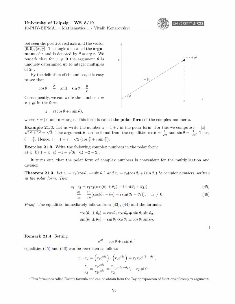
University of Leipzig – WS18/1910-PHY-BIPMA1 – Mathematics 1 / Vitalii Konarovskyi
θ
z = x + yi
r = |z|
y
x
between the positive real axis and the vector(0, 0), (x, y). The angle θ is called the argu-ment of z and is denoted by θ = arg z. Weremark that for z 6= 0 the argument θ isuniquely determined up to integer multiplesof 2π.
By the definition of sin and cos, it is easyto see that
cos θ =x
rand sin θ =
y
r.
Consequently, we can write the number z =x+ yi in the form
z = r(cos θ + i sin θ),
where r = |z| and θ = arg z. This form is called the polar form of the complex number z.
Example 21.3. Let us write the number z = 1 + i in the polar form. For this we compute r = |z| =√12 + 12 =
√2. The argument θ can be found from the equalities cos θ = 1√
2and sin θ = 1√
2. Thus,
θ = π4 . Hence, z = 1 + i =
√2(cos π4 + i sin π
4
).
Exercise 21.9. Write the following complex numbers in the polar form:a) i; b) 1− i; c) −1 +
√3i; d) −2− 2i.
It turns out, that the polar form of complex numbers is convenient for the multiplication anddivision.
Theorem 21.3. Let z1 = r1(cos θ1+ i sin θ1) and z2 = r2(cos θ2+ i sin θ2) be complex numbers, writtenin the polar form. Then
z1 · z2 = r1r2(cos(θ1 + θ2) + i sin(θ1 + θ2)), (45)z1z2
=r1r2
(cos(θ1 − θ2) + i sin(θ1 − θ2)), z2 6= 0. (46)
Proof. The equalities immediately follows from (43), (44) and the formulas
cos(θ1 ± θ2) = cos θ1 cos θ2 ∓ sin θ1 sin θ2,
sin(θ1 ± θ2) = sin θ1 cos θ2 ± cos θ1 sin θ2.
Remark 21.4. Settingeiθ = cos θ + i sin θ, 1
equalities (45) and (46) can be rewritten as follows
z1 · z2 =(r1e
iθ1)·(r2e
iθ2)
= r1r2ei(θ1+θ2),
z1z2
=r1e
iθ1
r2eiθ2=r1r2ei(θ1−θ2), z2 6= 0.
1This formula is called Euler’s formula and can be obtain from the Taylor expansion of functions of complex argument.
95
University of Leipzig – WS18/1910-PHY-BIPMA1 – Mathematics 1 / Vitalii Konarovskyi
Exercise 21.10. Simplify the expression cos θ+i sin θcosϕ−i sinϕ .
Exercise 21.11. Compute (1−√3i)(cos θ+i sin θ)
2(1−i)(cos θ−i sin θ) .
Corollary 21.1 (De Moivre’s formula). Let z = r(cos θ+ i sin θ) 6= 0 be a complex number. Then foreach n ∈ Z
zn = rn(cosnθ + i sinnθ).
Proof. The corollary immediately follows from Theorem 21.3.
Exercise 21.12. Compute: a) (1 + i)25; b) (√
3− 3i)15; c)(1+√3i
1−i
)20; d)
(1−
√3−i2
)24.
21.4 Roots of Complex Numbers
Let n ∈ N be fixed.
Definition 21.4. A complex number w is called an n-th root of z ∈ C if wn = z.
Theorem 21.4. Let z = r(cos θ+ i sin θ) 6= 0 be a complex number. Then z has n different n-th rootsgiven by the formula
wk = n√r
(cos
θ + 2πk
n+ i sin
θ + 2πk
n
), k = 0, 1, . . . , n− 1,
where n√r is the usual n-th root of the positive real number r.
Proof. Let w = ρ(cosϕ + i sinϕ) be a complex number written in the polar form such that wn = z.Then
wn = ρn(cosnϕ+ i sinnϕ) = r(cos θ + i sin θ),
by Corollary 21.1. Thus, ρn = r and nϕ = θ + 2πk, k ∈ Z. This implies that ρ = n√r and ϕ = θ+2πk
n ,k ∈ Z. So, we obtain that the numbers
wk = n√r
(cos
θ + 2πk
n+ i sin
θ + 2πk
n
), k ∈ Z,
are n-th roots of z. By the periodicity of sin and cos, one can see that there are only n different wk,k = 0, . . . , n− 1.
Example 21.4. Let us compute 4-th root of z = −1. First we write −1 in the polar form:−1 = 1(cosπ + i sinπ). Then wk = cos π+2πk
4 + i sin π+2πk4 , k = 0, 1, 2, 3, are 4-th roots of −1, by
Theorem 21.4. Thus, w0 = cos π4 + i sin π4 = 1√
2+ 1√
2i, w1 = cos π+2π
4 + i sin π+2π4 = − 1√
2+ 1√
2i,
w2 = cos π+4π4 + i sin π+4π
4 = − 1√2− 1√
2i, w3 = cos π+6π
4 + i sin π+6π4 = 1√
2− 1√
2i.
Remark 21.5. The n-th roots of z 6= 0 form a regular n-gon in the complex plane with center 0. Thevertices of this n-gon lie on the circle with center 0 and the radius n
√|z|.
Exercise 21.13. Solve the following equations:a) z5 − 2 = 0; b) z4 + i = 0; c) z3 − 4i = 0.
Exercise 21.14. Compute a) 6-th roots of 1−i√3+i
; b) 8-th roots of 1+i√3−i .
96
University of Leipzig – WS18/1910-PHY-BIPMA1 – Mathematics 1 / Vitalii Konarovskyi
22 Lecture 22 – Fundamental Theorem of Algebra and Definitionof Vector Space
22.1 Fundamental Theorem of Algebra
For more details see [3, Chapter 4].Let n ∈ N and a0, a1, . . . , an be a complex numbers. We set
f(z) = anzn + an−1z
n−1 + . . .+ a1z + a0, z ∈ C.
The function f is called a polynomial function. The numbers a0, a1, . . . , an are coefficients of thepolynomial f . If an 6= 0, then the number n is called the degree of f and is denoted by deg f := n.
In this section, we are going to prove that the equation f(z) = 0 as at most n solutions. The nexttheorem is called the fundamental theorem of algebra and we formulate it without prof. The prof willbe given at the course of complex analysis using Liouville’s theorem.
Theorem 22.1 (Fundamental theorem of algebra). For every n ∈ N and a0, a1, . . . , an ∈ C, an 6= 0,the equation
anzn + an−1z
n−1 + . . .+ a1z + a0 = 0
has at least one solution in C.
Theorem 22.2. Let f be a polynomial function of degree n ∈ N. Then
1) for any w ∈ C we have that f(w) = 0 iff there exists a polynomial g of degree n− 1 such that
f(z) = (z − w)g(z), z ∈ C;
2) there exist at most n distinct complex solutions of the polynomial equation f(z) = 0;
3) there exist w1, . . . , wn ∈ C (not necessary distinct) such that
f(z) = an(z − w1) . . . (z − wn), z ∈ C,
where an denotes the coefficient about zn.
Proof. To prove 1), we first recall that for each a, b ∈ R
an − bn = (a− b)(an−1 + an−2b+ . . .+ abn−2 + bn−1) = (a− b)n∑k=1
an−kbk−1.
Let f(w) = 0. Then
f(z) = f(z)− f(w) = an(zn − wn) + an−1(zn−1 − wn−1) + . . .+ a1(z − w)
= an(z − w)n∑k=1
zn−kwk−1 + an−1(z − w)n−1∑k=1
zn−k−1wk−1 + . . .+ a1(z − w)
= (z − w)
(an
n∑k=1
zn−kwk−1 + an−1
n−1∑k=1
zn−k−1wk−1 + . . .+ a1
)= (z − w)g(z),
97
University of Leipzig – WS18/1910-PHY-BIPMA1 – Mathematics 1 / Vitalii Konarovskyi
where g(z) = an∑n
k=1 zn−kwk−1 + an−1
∑n−1k=1 z
n−k−1wk−1 + . . .+ a1, z ∈ C, is a polynomial of degreen− 1.
Now, we prove 3). Let w1 be a complex number such that f(w1) = 0, which exists according toTheorem 22.1. Applying the part 1) of Theorem 22.2, we have that there exists a polynomial g1 suchthat f(z) = (z−w1)g1(z), z ∈ C. Next, using Theorem 22.1 again, we obtain that there exists w2 suchthat f(w2) = 0. By Theorem 22.2 1), there exists a polynomial g2 such that g1(z) = (z − w2)g2(z),z ∈ C. Consequently, f(z) = (z − w1)(z − w2)g2(z), z ∈ C. Applying theorems 22.1 and 22.2 1) ntimes, we get that
f(z) = (z − w1) . . . (z − wn)gn, z ∈ C, (47)
for some w1, w2, . . . , wn ∈ C and a polynomial gn of degree 0 which is a constant function. Since theright hand side of (47) is a polynomial with the coefficient gn about zn, we can conclude that gn = an.
The part 2) of the theorem easily follows from 3).
Exercise 22.1. For a complex number α show that the coefficients of the polynomial
p(z) = (z − α)(z − α)
are real numbers.
Exercise 22.2. Let p(z) be a polynomial with real coefficients and let α be a complex number. Provethat p(α) = 0 if and only if p(α) = 0.
Exercise 22.3. Prove that any polynomial p(z) with real coefficients can be decomposed into aproduct of polynomials of the form az2 + bz + c, where a, b, c ∈ R.
22.2 Definition and some Examples of Vector Spaces
For more details see [3, Chapter 5].Let F denote the set of real numbers R or complex numbers C. We will call F a field. We also
consider a set V , whose elements are called vectors and will be denoted by v,u,w . . . etc. We defineon V two operations:
• vector addition + : V × V → V , that maps two elements u,v of V to u + v ∈ V ;
• scalar multiplication · : F× V → V , that maps a ∈ F and u ∈ V to a · u = au ∈ V .
Definition 22.1. A vector space over F is a set V together with operations of vector addition andscalar multiplication which satisfy the following properties:
1) commutativity: u + v = v + u for all u,v ∈ V ;
2) associativity: (u + v) + w = u + (v + w) and (ab)v = a(bv) for all a, b ∈ F and u,v,w ∈ V ;
3) additive identity: there exists a vector 0 ∈ V such that 0 + v = v for all v ∈ V ;
4) additive inverse: for every v ∈ V there exists a vector w ∈ V (denoted by −v) such thatv + w = 0;
5) multiplicative identity: 1 · v = v for all v ∈ V ;
98
University of Leipzig – WS18/1910-PHY-BIPMA1 – Mathematics 1 / Vitalii Konarovskyi
6) distributivity: a(u + v) = au + av and (a+ b)v = av + bv for all a, b ∈ F, u,v ∈ V .
A vector space over R will be called a real vector space and a vector space over C is similarlycalled a complex vector space.
Example 22.1. The set V = F with the usual operations of addition and multiplication is trivially avector space over F.
Example 22.2. The set
Fn = {x = (x1, x2, . . . , xn) : xk ∈ F, k = 1, . . . , n}
with operationsx + y = (x1 + y1, x2 + y2, . . . , xn + yn)
andax = (ax1, ax2, . . . , axn),
for all a ∈ F, x = (x1, x2, . . . , xn), y = (y1, y2, . . . , yn) ∈ Fn, is a vector space. It is easily tosee that the additive identity is 0 = (0, 0, . . . , 0) and the additive inverse of x = (x1, x2, . . . , xn) is−x = (−x1,−x2, . . . ,−xn).
Example 22.3. Similarly, the set
F∞ = {x = (x1, x2, . . .) : xk ∈ F, k ∈ N}
with operationsx + y = (x1 + y1, x2 + y2, . . .)
andax = (ax1, ax2, . . .),
for all a ∈ F, x = (x1, x2, . . .), y = (y1, y2, . . .) ∈ F∞, is also a vector space, where 0 = (0, 0, . . .) isadditive identity and −x = (−x1,−x2, . . .) is the additive inverse of x = (x1, x2, . . .).
Example 22.4. The set of all polynomials of degree at most n
Fn[z] = {p(z) = anzn + . . .+ a1z + a0, z ∈ F : ak ∈ F, k = 1, . . . , n}
with the addition
(p + q)(z) = (an + bn)zn + . . .+ (a1 + b1)z + a0 + b0, z ∈ F,
and scalar multiplication
(ap)(z) = aanzn + . . .+ aa1z + aa0, z ∈ F,
for all a ∈ F and p(z) = anzn + . . .+ a1z + a0, q(z) = bnz
n + . . .+ b1z + b0, z ∈ F, from Fn[z] is alsoa vector space.
Exercise 22.4. The vector space F[z] of all polynomials of any degree can be defined similarly asFn[z] and is also a vector space.
99
University of Leipzig – WS18/1910-PHY-BIPMA1 – Mathematics 1 / Vitalii Konarovskyi
Example 22.5. The set of (real-valued) continuous functions on an interval [a, b] with the usualaddition of functions and multiplication by a constant is a real vector space.
Exercise 22.5. The set of complex numbers C = {x + iy : x, y ∈ R} can be considered as a realvector space with the usual addition of complex numbers and the multiplication by the real number.
Example 22.6. The set V = {0}, where 0 is any element, with addition 0 + 0 := 0 and scalarmultiplication a · 0 := 0 is a vector space. (Here 0 also plays a role of the additive identity).
Exercise 22.6. Show that the sets from the previous examples are vector spaces under correspondingaddition and scalar multiplication.
Exercise 22.7. For each of the following sets, either show that the set is a vector space over F orexplain why it is not a vector space.
a) The set R of real numbers under the usual operations of addition and multiplication, F = R.
b) The set R of real numbers under the usual operations of addition and multiplication, F = C.
c) The set {f ∈ C[0, 1] : f(0) = 2} under the usual operations of addition and multiplication offunctions, F = R.
d) The set {f ∈ C[0, 1] : f(0) = f(1) = 0} under the usual operations of addition and multiplicationof functions, F = R.
e) The set {(x, y, z) ∈ R3 : x−2y+z = 0} under the usual operations of addition and multiplicationon R3, F = R.
f) The set {(x, y, z) ∈ C3 : 2x+z+i = 0} under the usual operations of addition and multiplicationon C3, F = C.
22.3 Elementary Properties of Vector Spaces
In this section, we prove some important and simple properties of vector spaces. Let V denote a vectorspace over F.
Proposition 22.1. Any vector space has a unique additive identity.
Proof. Let us assume that there exist two additive identities 0 and 0′. Then
0 = 0 + 0′ = 0′,
where the first identity holds since 0′ is an identity and the second equality holds since 0 is anidentity.
Proposition 22.2. Every v ∈ V has a unique inverse.
Proof. We assume that w and w′ are additive inverses of v so that v + w = 0 and v + w′ = 0. Then
w = w + 0 = w + (v + w′) = (w + v) + w′ = 0 + w′ = w′.
100
University of Leipzig – WS18/1910-PHY-BIPMA1 – Mathematics 1 / Vitalii Konarovskyi
Since the additive inverse of v is unique, we will denote it by −v. We also define w−v := w+(−v).
Proposition 22.3. For every v ∈ V 0 · v = 0.
Proof. For v ∈ V we have that
0 · v = (0 + 0) · v = 0 · v + 0 · v.
Adding the additive inverse of 0v to both sides, we obtain
0 = 0v − 0v = (0v + 0v)− 0v = 0v.
Proposition 22.4. For every a ∈ F a · 0 = 0.
Exercise 22.8. Prove Proposition 22.4.
Proposition 22.5. For every v ∈ V (−1) · v = −v.
We recall that the vector −v denotes the additive inverse of v.
Proof. For v ∈ V , we have
v + (−1) · v = 1 · v + (−1) · v = (1 + (−1))v = 0 · v = 0,
by Proposition 22.3.
101
University of Leipzig – WS18/1910-PHY-BIPMA1 – Mathematics 1 / Vitalii Konarovskyi
23 Lecture 23 – Vector Subspaces and Span
23.1 Vector Subspaces
Throughout this section, V denotes a vector space over F.
Definition 23.1. Let V be a vector space over F, and let U ⊂ V be a subset of V . Then U is calleda subspace of V if U is a vector space over F
To check that a subset U ⊂ V is a subspace, it is suffices to check only a few of the conditions ofa vector space.
Lemma 23.1. Let U ⊂ V be a subset of a vector space V over F. Then U is a subspace of V iff thefollowing conditions holds:
(1) closure under addition: u,v ∈ U implies u + v ∈ U ;
(2) closure under scalar multiplication: a ∈ F, u ∈ U implies that au ∈ U .
Exercise 23.1. Prove Lemma 23.1.
Example 23.1. In every vector space V , the subset U = {0} is a vector subspace of V .
Exercise 23.2. Show that the set {(x1, 0) : x1 ∈ R} is a vector subspace of R2.
Exercise 23.3. Show that the set {(x1, x2, x3) ∈ R3 : x1 + 2x2−x3 + 1 = 0} is not a vector subspaceof R3.
Exercise 23.4. Let U1 and U2 be a vector subspaces of V . Prove that the intersection U1 ∩U2 is alsoa vector subspace. Is the union U1 ∪ U2 a vector subspace?
23.2 Sums and Direct Sums of Vector Subspaces
Let U1, U2 be a vector subspaces of V .
Definition 23.2. Let U1, U2 be a vector subspaces of V . The set
U1 + U2 = {u1 + u2 : u1 ∈ U1, u2 ∈ U2}
is said to be a sum of vector subspaces U1 and U2.
Exercise 23.5. Check that a direct sum of two vector subspaces is a vector space.
Example 23.2. Let
U1 = {(x, 0, 0) ∈ F3 : x ∈ F}U2 = {(0, y, 0) ∈ F3 : y ∈ F}U3 = {(y, y, 0) ∈ F3 : y ∈ F}.
ThenU1 + U2 = U1 + U3 = {(x, y, 0) ∈ F3 : x, y ∈ F}.
102
University of Leipzig – WS18/1910-PHY-BIPMA1 – Mathematics 1 / Vitalii Konarovskyi
We remark that u ∈ U = U1 +U2 if and only if there exist vectors u1 ∈ U1 and u2 ∈ U2 such thatu = u1 + u2.
Definition 23.3. If every vector u ∈ U = U1 +U2 can be uniquely written as u = u1 +u2 for u1 ∈ U1
and u2 ∈ U2. Then we call the vector space U the direct sum of U1, U2 and denote by
U = U1 ⊕ U2.
Example 23.3. Let
U1 = {(x, y, 0) ∈ R3 : x, y ∈ R},U2 = {(0, 0, z) ∈ R3 : z ∈ R},U3 = {(0, y, z) ∈ R3 : y, z ∈ R}.
Then R3 = U1 ⊕ U2. But R3 = U1 + U3 and R3 6= U1 ⊕ U3 (the vector (0, 0, 0) can be written as(0, 0, 0) + (0, 0, 0) and (0,−1, 0) + (0, 1, 0)).
Proposition 23.1. Let U1 and U2 be a vector subspaces of V . Then V = U1 ⊕ U2 iff the followingconditions hold:
(1) V = U1 + U2;
(2) If 0 = u1 + u2 with u1 ∈ U1 and u2 ∈ U2, then u1 = u2 = 0.
Proof. We assume that V = U1 ⊕ U2. Then Condition (1) follows from the definition. Since 0 can beuniquely written as 0 + 0, we have that Condition (2) is also true.
Next, let conditions (1) and (2) hold. By Condition (1), for every vector u ∈ V there exist u1 ∈ U1
and u2 ∈ U2 such that u = u1 + u2. We assume that u = v1 + v2 for some v1 ∈ U1 and v2 ∈ U2.Subtracting the two equations, we obtain
0 = (u1 − v1) + (u2 − v2),
where u1 − v1 ∈ U1 and u2 − v2 ∈ U2. By Condition (2), we have that u1 = v1 and u2 = v2. Thisimplies that V = U1 ⊕ U2.
Proposition 23.2. Let U1 and U2 be a vector subspaces of V . Then V = U1 ⊕ U2 iff the followingconditions hold:
(1) V = U1 + U2;
(2) U1 ∩ U2 = {0}.
Proof. We assume that V = U1⊕U2. Then Condition (1) follows from the definition. Next, we supposethat u ∈ U1∩U2. Then by Exercise 23.4, −u also belongs to U1∩U2 because U1∩U2 is a vector space.Thus, 0 = u + (−u), where u ∈ U1 ∩ U2 ⊂ U1 and −u ∈ U1 ∩ U2 ⊂ U2. By Proposition 23.1, u = 0.
Next, we assume that conditions (1) and (2) hold. In order to prove that V = U1 ⊕ U2, we showthat 0 = u1 +u2, where u1 ∈ U1 and u2 ∈ U2, implies u1 = u2 = 0. Since 0 = u1 +u2, u1 = −u2. So,u1 = −u2 ∈ U2 because U2 is a vector space. Thus, u1 ∈ U1 ∩ U2 and, consequently, u1 = −u2 = 0,according to Condition (2). USsing Proposition 23.1, we obtain that V is the direct sum of U1 andU2.
103
University of Leipzig – WS18/1910-PHY-BIPMA1 – Mathematics 1 / Vitalii Konarovskyi
Exercise 23.6. Prove or give a counterexample to the following claim:
1) Let V be a vector space over F and suppose that W1, W2 and W3 are vector subspaces of V suchthat W1 +W3 = W2 +W3. Then W1 = W2.
2) Let V be a vector space over F and suppose that W1, W2 and W3 are vector subspaces of V suchthat W1 ⊕W3 = W2 ⊕W3. Then W1 = W2.
Exercise 23.7. Let F[z] denote the vector space of all polynomials with coefficients in F and let
U = {az2 + bz5 : a, b ∈ F}.Find a subspace W of F[z] such that F [z] = U ⊕W .
23.3 Linear Span
In order to give a definition of one of the main notion of the linear algebra: basis of a vector space,we need to introduce a notion of a linear span of vectors.
Definition 23.4. A vector v ∈ V is a linear combination of vectors v1,v2, . . . ,vn, if there existsscalars a1, a2, . . . , an from F such that
v = a1v1 + a2v2 + . . .+ anvn.
Definition 23.5. The set
span{v1,v2, . . . ,vn} := {a1v1 + a2v2 + . . .+ anvn : a1, a2, . . . , an ∈ F}is called a linear span of vectors v1,v2, . . . ,vn.
The following lemma follows from the definitions of a vector spaces and linear span.
Proposition 23.3. Let V be a vector space and v1,v2, . . . ,vn ∈ V . Then
(i) the vector vi belongs to span{v1,v2, . . . ,vn};
(ii) span{v1,v2, . . . ,vn} is a subspace of V ;
(iii) If U is a subspace of V such that v1,v2, . . . ,vn ∈ U , then span{v1,v2, . . . ,vn} ⊂ U .
Proposition 23.3 implies that span{v1,v2, . . . ,vn} is the smallest vector space of V which containsthe set of vectors v1,v2, . . . ,vn.
Definition 23.6. If span{v1,v2, . . . ,vn} = V , then we say that vectors v1,v2, . . . ,vn span V andwe call V finite-dimensional. If a vector space is not finite dimensional, then we call it infinite-dimensional.
Example 23.4. The vectors e1 = (1, 0, 0, . . . , 0), e2 = (0, 1, 0, . . . , 0), ..., en = (0, . . . , 0, 1) span Fn.According to the previous definition the space Fn is finite-dimensional.
Example 23.5. Let pk(z) = zk, for k = 0, . . . , n. Then the set p0,p1,p2, . . . ,pn span Fn[z]. It iseasy to see that the space F[z] of all polynomials is infinite-dimensional.
Exercise 23.8. Consider the complex vector space V = C3 and the list {v1,v2,v3} of vectors in V ,where v1 = (i, 0, 0), v2 = (i, 1, 0) and v3 = (i, i,−1).a) Prove that span{v1,v2,v3} = V .
104
University of Leipzig – WS18/1910-PHY-BIPMA1 – Mathematics 1 / Vitalii Konarovskyi
24 Lecture 24 – Basis
24.1 Linear Independence
In this section, we are going to define the notion of linear independence of a list of vectors.
Definition 24.1. Vectors v1,v2, . . . ,vn are called linearly independent if the only solution fora1, a2, . . . , an ∈ F to the equation
a1v1 + a2v2 + . . .+ anvn = 0
is a1 = a2 = . . . = an = 0. Otherwise, the vectors v1, v2, . . . , vn are said to be linearly dependent.
Example 24.1. The vectors e1, e2, . . . , en from Example 23.4 are linearly independent, since
a1e1 + a2e2 + . . .+ anen = (a1, a2, . . . , an) = (0, 0, . . . , 0)
provided a1 = a2 = . . . = an = 0.
Example 24.2. The vectors v1 = (1, 1, 3), v2 = (1, 1, 0), v3 = (0, 0, 1) are linearly dependent because
v1 − v2 − 3v3 = (0, 0, 0).
Example 24.3. The vectors (1, z, z2, . . . , zn) in Fn[z] are linearly independent.
Exercise 24.1. Show that the vectors v1 = (1, 1, 1), v2 = (1, 2, 3), and v3 = (2,−1, 1) are linearlyindependent in R3. Write v = (1,−2, 5) as a linear combination of v1, v2 and v3.
Exercise 24.2. Consider the complex vector space V = C3 and the vectors v1 = (i, 0, 0), v2 = (i, 1, 0),v3 = (i, i,−1).a) Prove that span{v1,v2,v3} = V .b) Are v1,v2,v3 a basis of C3?
Exercise 24.3. Determine the value of λ ∈ R for which each vectors (λ,−1,−1), (−1, λ,−1),(−1,−1, λ) are linearly dependent in R3.
Theorem 24.1. Vectors v1,v2, . . . ,vn are linearly independent iff each vector v ∈ span{v1,v2, . . . ,vn}can be unequally written as a linear combination of v1,v2, . . . ,vn.
Proof. Let v1,v2, . . . ,vn be linearly independent. If v ∈ span{v1,v2, . . . ,vn} can be written as
v = a1v1 + a2v2 + . . .+ anvn = a′1v1 + a′2v2 + . . .+ a′nvn,
then 0 = v− v = (a1 − a′1)v1 + (a2 − a′2)v2 + . . .+ (an − a′n)vn, which implies that a1 = a′1, a2 = a′2,..., an = a′n. The sufficiency can be proved trivially, taking v = 0.
Theorem 24.2. Let v1,v2, . . . ,vn be linearly dependent and v1 6= 0. Then there exists j ∈ {2, . . . , n}such that
1) vj ∈ span{v1,v2, . . . ,vj−1};
2) span{v1, . . . ,vj−1,vj+1, . . . ,vn} = span{v1,v2, . . . ,vn}.
105
University of Leipzig – WS18/1910-PHY-BIPMA1 – Mathematics 1 / Vitalii Konarovskyi
Proof. Since v1,v2, . . . ,vn are linearly dependent, there exist a1, a2, . . . , an ∈ F such that a1v1 +a2v2 + . . . + anvn = 0. Since v1 6= 0, not all of a2, . . . , an are 0. Let j ∈ {2, . . . , n} be the largestindex such that aj 6= 0. Then we have
vj = −a1aj
v1 −a2aj
v2 − . . .−aj−1aj
vj−1. (48)
This implies 1).Let v be an arbitrary vector from span{v1,v2, . . . ,vn}. It means that there exist b1, b2, . . . , bn ∈ F
such thatv = b1v1 + b2v2 + . . .+ bnvn.
According to (48), v can be rewritten as linear combination of the vectors v1, . . . ,vj−1,vj+1, . . . ,vn.This proves 2).
Theorem 24.3. Let V be a finite-dimensional vector space, v1,v2, . . . ,vn be linearly independent andspan V , and let w1,w2, . . . ,wm be vectors that span V . Then n ≤ m.
Proof. For the proof of the theorem see the proof of Theorem 5.2.9 [3].
Exercise 24.4. Let V be a vector space over F, and suppose that v1,v2, . . . ,vn ∈ V are linearlyindependent. Let w be a vector from V such that the vectors v1 + w,v2 + w, . . . ,vn + w are linearlydependent. Prove that w ∈ span{v1,v2, . . . ,vn}.
24.2 Bases
Definition 24.2. A set of vectors {v1,v2, . . . ,vn} is a basis of a finite-dimensional vector space V ifv1,v2, . . . ,vn are linearly independent and span V , i.e. V = span{v1,v2, . . . ,vn}.
Remark 24.1. We remark that each vector v ∈ V can be uniquely written as a linear combinationof v1,v2, . . . ,vn iff {v1,v2, . . . ,vn} is a basis of V .
Example 24.4. The set of the vectors {e1, e2, . . . , en} is a basis of Fn.
Exercise 24.5. Prove that the set of vectors (1, 1, 0), (1, 0, 0), (0, 0, 1) is a basis of F3.
Example 24.5. The set 1, z2, . . . , zn is a basis of Fn[z].
Theorem 24.4 (Basis reduction theorem). If V = span{v1,v2, . . . ,vn}, then either the set {v1,v2, . . . ,vn}is a basis of V or some vk can be removed to obtain a basis of V .
Proof. Suppose V = span{v1,v2, . . . ,vn}. We start with the set S = {v1,v2, . . . ,vn} and sequentiallyrun through all vectors vk for k = 1, 2, . . . ,m to determine whether to keep or remove them from S:
Step 1. If v1 = 0, then remove v1 from S. Otherwise, leave S unchanged.Step k. If vk ∈ span{v1,v2, . . . ,vk−1}, then remove vk from S. Otherwise, leave S unchanged.The final set S still spans V since, at each step, a vector was only discarded if it was already in the
span of the previous vectors. The process also ensures that no vector is in the span of the previousvectors. Hence, by Theorem 24.2, the final list S is linearly independent. It follows that S is a basisof V .
106
University of Leipzig – WS18/1910-PHY-BIPMA1 – Mathematics 1 / Vitalii Konarovskyi
Example 24.6. The set of vectors v1 = (1,−1, 0), v2 = (0, 1, 0), v3 = (1, 1, 1), v4 = (0,−1, 2) arelinearly dependent, since
0v1 + 3v2 − 2v3 + v4 = 0.
But the vectors v1,v2,v3 form a basis of R3. Indeed, each element v = (x, y, z) can be uniquelywritten as follows
(x, y, z) = (x− z)v1 + (x+ y − 2z)v2 + zv3.
Corollary 24.1. Every finite-dimensional vector space has a basis.
Proof. The statement immediately follows from Theorem 24.4.
Theorem 24.5 (Basis Extension Theorem). Every linearly independent set of vectors in a finite-dimensional vector space V can be extended to a basis of V .
Proof. Let V be finite-dimensional and v1,v2, . . . ,vn be linearly independent. Since V is finite-dimensional, there exists a set of vectors w1,w2, . . . ,wm that spans V . We are going to adjoin someof the wk to {v1,v2, . . . ,vn} in order to create a basis of V .
Step 1. If w1 ∈ span{v1,v2, . . . ,vn}, then let S := {v1,v2, . . . ,vn}. Otherwise, S := span{v1,v2, . . . ,vn, w1}.Step k. If wk ∈ spanS, then leave S unchanged. Otherwise, adjoin wk to S.After each step, the set S is still linearly independent, since we only adjoined wk if wk was not
in the span of the previous vectors. After m steps, wk ∈ spanS for all k = 1, 2, . . . ,m. Since the set{w1,w2, . . . ,wm} spans V , S also spans V . Consequently, S is a basis of V .
24.3 Dimension
Let {v1,v2, . . . ,vn} and {w1,w2, . . . ,wm} be two bases of a finite-dimensional vector space V , thatis, they both are linearly independent and span V . Then by Theorem 24.3, it follows that n = m.
Definition 24.3. We call the length of any basis of V the dimension of V and denote by dimV .
Example 24.7. According to Example 24.4, the dimension of Fn equals n.
Example 24.8. By Example 24.5, the dimension of Fn[z] equals n+ 1.
Exercise 24.6. Let p0,p1, . . . ,pn ∈ Fn[z] satisfy pj(2) = 0 for all j = 0, 1, . . . , n. Prove thatp0,p1, . . . ,pn must be a linearly dependent in Fn[z].
Remark 24.2. We note that dimCn = n as a complex vector space, whereas dimCn = 2n as a realvector space. This comes from the fact that we can view C itself as a real vector space of dimension2 with basis {1, i}.
Theorem 24.6. Let V be a finite-dimensional vector space with dimV = n. Then
(i) If U ⊂ V is a subspace of V , then dimU ≤ dimV .
(ii) If V = span{v1,v2, . . . ,vn}, then {v1,v2, . . . ,vn} is a basis of V .
(iii) If v1,v2, . . . ,vn are linearly independent in V , then they form a basis of V .
107
University of Leipzig – WS18/1910-PHY-BIPMA1 – Mathematics 1 / Vitalii Konarovskyi
Proof. To prove statement (i), first we note that U is necessarily finite-dimensional (otherwise wecould find a list of linearly independent vectors longer than dimV ). Therefore, by Corollary 24.1, Uhas a basis u1,u2, . . . ,um which are linearly independent in both U and V . By Theorem 24.5, we canextend u1,u2, . . . ,um to a basis of V , which is of length n since dimV = n. This implies that m ≤ n.
In order to prove statement (ii), we suppose that v1,v2, . . . ,vn span V . Then, by the basisreduction theorem (see Theorem 24.4), this set can be reduced to a basis. However, every basisof V has length n. Hence, no vector needs to be removed from {v1,v2, . . . ,vn}. It follows that{v1,v2, . . . ,vn} is a basis of V .
To prove statement (iii), we assume that v1,v2, . . . ,vn are linearly independent. By the basisextension theorem (see Theorem 24.5), this set can be extended to a basis. However, every basis haslength n. Hence, no vector needs to be added to {v1,v2, . . . ,vn}. It follows that {v1,v2, . . . ,vn} is abasis of V .
Theorem 24.7. Let U ⊂ V be a subspace of a finite-dimensional vector space V . Then there exists asubspace W ⊂ V such that V = U ⊕W .
Proof. Let u1,u2, . . . ,um be a basis of U . By Theorem 24.6 (i), we know that m ≤ dimV . Hence, bythe basis extension theorem (see Theorem 24.5), the set {u1,u2, . . . ,um} can be extended to a basis{u1,u2, . . . ,um,w1,w2, . . . ,wk} of V . Let W := span{w1,w2, . . . ,wk}.
We now show that V = U ⊕W . Since the set {u1,u2, . . . ,um,w1,w2, . . . ,wk} is a basis of V , eachelement v of V can be uniquely written as follows
v = a1u1 + a2u2 + . . .+ amum + b1w1 + b2w2 + . . .+ bkwk = u + w
for some a1, a2, . . . , am, b1, b2, . . . , bk ∈ F, where u := a1u1+a2u2+ . . .+amum and w = b1w1+b2w2+. . .+bkwk. Since u ∈ U and w ∈W , V is the direct sum of U and W , according to Definition 23.3.
Exercise 24.7. Let V be a finite-dimensional vector space over F with dimV = n for some n ∈ N.Prove that there exist n one-dimensional subspaces U1, U2, . . . , Un of V such that
V = U1 ⊕ U2 ⊕ . . .⊕ Un.
Theorem 24.8. If U,W ⊂ V are subspaces of a finite-dimensional vector space, then
dim(U +W ) = dimU + dimW − dim(U ∩W ).
Proof. For the proof of the theorem see the proof of Theorem 5.4.6 [3].
Exercise 24.8. Let V be a finite-dimensional vector space over F, and let U be a vector subspace ofV for which dimU = dimV . Prove that U = V .
108
University of Leipzig – WS18/1910-PHY-BIPMA1 – Mathematics 1 / Vitalii Konarovskyi
25 Lecture 25 – Linear Maps
109
University of Leipzig – WS18/1910-PHY-BIPMA1 – Mathematics 1 / Vitalii Konarovskyi
26 Lecture 26 – Matrices
110
University of Leipzig – WS18/1910-PHY-BIPMA1 – Mathematics 1 / Vitalii Konarovskyi
References
[1] K.A. Ross. Elementary Analysis: The Theory of Calculus. Undergraduate Texts in Mathematics.Springer New York, 2013.
[2] Walter Rudin. Principles of mathematical analysis. McGraw-Hill Book Co., New York-Auckland-Dusseldorf, third edition, 1976. International Series in Pure and Applied Mathematics.
[3] I. Lankham, B. Nachtergaele, and A. Schilling. Linear Algebra As An Introduction To AbstractMathematics. WSPC, 2016.
111
University of Leipzig – WS18/1910-PHY-BIPMA1 – Mathematics 1 / Vitalii Konarovskyi
A Selected exercises
1. Show that
a) A ∪ ∅ = A, A ∪A = A, A ∪B = B ∪A, A ∪ (B ∪ C) = (A ∪B) ∪ C =: A ∪B ∪ C;
b) A ∩ ∅ = ∅, A ∩A = A, A ∪B = B ∩A, A ∩ (B ∩ C) = (A ∩B) ∩ C =: A ∩B ∩ C;
c) A4B = (A ∪B) \ (A ∩B) = (A \B) ∪ (B \A), A \B = A ∩Bc;
d) A ∩ (B ∪ C) = (A ∩B) ∪ (A ∩ C), A ∪ (B ∩ C) = (A ∪B) ∩ (A ∪ C).
e) (A ∪B)c = Ac ∩Bc, (A ∩B)c = Ac ∪Bc.
2. Let An = {1, . . . , n} for each n ∈ N. Then
⋃n∈N
An =
∞⋃n=1
An = N,⋂n∈N
An =
∞⋂n=1
An = {1}.
3. Prove thata)√
6 6∈ Q; b)√
2 +√
3 6∈ Q; c) for each n ∈ N either√n ∈ N or
√n 6∈ Q.
4. Using mathematical induction prove that:a) 1 + 2 + · · ·+ n = 1
2n(n+ 1) for positive integers n;b) 13 + 23 + . . .+ n3 = (1 + 2 + . . .+ n)2 for each n ∈ N;c) 11n − 4n is divisible by 7 for each n ∈ N;d) 5n − 4n− 1, n ∈ N, are divisible by 16;e) 1 + 1
22+ . . .+ 1
n2 ≤ 2− 1n for all n ∈ N.
5. Prove that there does not exist a rational number x solving the equation x2 = 2.
6. Prove that the following sets are bounded:
a){
nn+1 : n ∈ N
};
b){
(−1)nn+1n−(−1)n : n ∈ N
}.
7. For each a < b prove that inf[a, b] = inf(a, b] = a and sup[a, b] = sup[a, b) = b.
8. Show thata) 2n ≥ n+ 1, n ∈ N; b) 3n ≥ 2n+ 1, n ∈ N; c) 2n > (
√2− 1)2n2, n ∈ N.
9. Let x1, . . . , xn be a positive real numbers. Prove that
(1 + x1) · . . . · (1 + xn) ≥ 1 + x1 + . . .+ xn.
10. Prove the boundedness of the following sequences:
a)(2n
n!
)n≥1; b)
an =
√2 +
√2 + . . .+
√2 +√
2︸ ︷︷ ︸n square roots
n≥1
.
112
University of Leipzig – WS18/1910-PHY-BIPMA1 – Mathematics 1 / Vitalii Konarovskyi
11. Prove the following statements:
a) an → a, n→∞ ⇔ an − a→ 0, n→∞ ⇔ |an − a| → 0, n→∞;
b) an → 0, n→∞ ⇔ |an| → 0, n→∞;
c) an → a, n→∞ ⇔ ∀ε > 0 ∃N ∈ N : {aN , aN+1, . . .} ⊂ (x− ε, x+ ε);
d) an → 0, n→∞ ⇔ sup{|ak| : k ≥ n} → 0, n→∞;
e) an → a, n→∞ ⇒ |an| → |a|, n→∞.
12. Prove that for a sequence (an)n≥1 with an 6= 0 the equality limn→∞
|an| = +∞ is equivalent to
limn→∞
1an
= 0.
13. Compute the following limits:a) lim
n→∞n3−2n2 cosn+n√
n−3n3+1; b) lim
n→∞(√n2 + n − √n); c) lim
n→∞n√n22n + 3n; d) lim
n→∞sin2 n√
n; e)
limn→∞
n2+sinnn2+n cosn
; f) limn→∞
2n+n3
3n+1 ; g) n+1√n.
14. Let (an)n≥1 be a bounded sequence and bn → 0, n ≥ ∞. Prove that anbn → 0, n→∞.
15. Let (an)n≥1 be a sequence such that ann → 0, n→∞. Prove that max{a1,a2,...,an}
n → 0, n→∞.
16. Let (an)n≥1 be a bounded sequence and bn → +∞, n ≥ ∞. Prove that an + bn → +∞, n→∞.
17. Using the monotonicity compute the following limits:
a) limn→∞
10n
n! = 0; b) limn→∞
n!
2n2; c) lim
n→∞
√2 +
√2 + . . .+
√2 +√
2︸ ︷︷ ︸n square roots
; d) limn→∞
n2√n = 0.
18. Identify the set of subsequential limits of the following sequences:a)(sin 2πn
3
)n≥1; b) (sin 3πn)n≥1; c) (an)n≥1,
where an =
{(−1)
n+12 + n, if n is odd,
(−1)n2 + 1
n , if n is even.
19. Prove that an → a, n→∞ ⇔ limn→∞
an = limn→∞
an = a.
20. For a sequence (an)n≥1 compute limn→∞
an and limn→∞
an, if for all n ≥ 1
a) an = 1− 1n ; b) an = (−1)n
n + 1+(−1)n2 ; c) an = n−1
n+1 cos 2nπ3 ; d) an = 1 + n sin nπ
2 ;
e) an =(1 + 1
n
)n · (−1)n + sin nπ4 ; f) an = (−1)n
n + 1+(−1)n2 .
21. Check whether the following sequences are Cauchy sequences.a)(
12n
)n≥1; b) ((−1)n)n≥1; c)
(an = sin 1
21+ sin 2
22+ . . .+ sinn
2n
)n≥1.
22. Show that (an)n≥1 is a Cauchy sequence iff supm≥N,n≥N
|am − an| → 0, N →∞.
23. Find the domain and the range of the following functions:a) f(x) = 1
(x+1)2; b) f(x) =
√1− x2; c) f(x) = ln(1 + x).
113
University of Leipzig – WS18/1910-PHY-BIPMA1 – Mathematics 1 / Vitalii Konarovskyi
24. Let f : X → Y and A1 ⊂ X, A2 ⊂ X. Check thata) f(A1∪A2) = f(A1)∪f(A2); b) f(A1∩A2) ⊂ (f(A1) ∩ f(A2)); c) (f(A1)\f(A2)) ⊂ f(A1\A2);d) A1 ⊂ A2 ⇒ f(A1) ⊂ f(A2); e) A1 ⊂ f−1(f(A1)); f) (f(X) \ f(A1)) ⊂ f(X \A1).
25. Let f : X → Y and B1 ⊂ Y , B2 ⊂ Y . Show thata) f−1(B1 ∪B2) = f−1(B1) ∪ f−1(B2); b) f−1(B1 ∩B2) = f−1(B1) ∩ f−1(B2);c) f−1(B1 \B2) = f−1(B1) \ f−1(B2); d) B1 ⊂ B2 ⇒ f−1(B1) ⊂ f−1(B2);e) f(f−1(B1)) = B1 ∩ f(X); f) f−1(Bc
1) = (f−1(B1))c.
26. Prove that the set of all limit points of Q equals R ∪ {−∞,+∞}.
27. Prove that 1f(x) → 0, x→ a, if f(x)→ +∞, x→ a.
28. Prove that the limit of the function f(x) = cos 1x , x ∈ R \ {0}, does not exist at the point a = 0.
29. Using ε− δ definition, show thata) lim
x→4
√x = 2; b) lim
x→+∞lnxx = 0.
30. Compute the following limits:a) lim
x→0
tanxx ; b) lim
x→0
1−cosxx2
; c) limx→1
x2−xx2−3x+2
; d) limx→+∞
x3−x sinx+x1−3x3+lnx
; e) limx→+∞
x2+cosx+1√x4+1+x+3
;
f) limx→0
(2
sin2 x− 1
1−cosx
); g) lim
x→0
x2+x3√1+sinx−1 ; h) lim
x→+∞
(x(√x2 + 2x+ 2− x− 1)
);
i) limx→+∞
(√ax+ 1−√x), for some a > 0.
31. Compute the following limits:
a) limx→0−
x√1−cos2 x ; b) lim
x→0+
x√1−cos2 x ; c) lim
x→π2−
x−π2√
1−sinx ; d) limx→π
2+
x−π2√
1−sinx ;
e) limx→0+
e−1x ; f) lim
x→0+
e−1x
x .
32. Let f be an increasing function on an interval [a, b].a) For each c ∈ (a, b) show that the one-sided limits f(a+), f(c−), f(c+), f(b−) exist.b) Check the inequalities
f(a) ≤ f(a+) ≤ f(c−) ≤ f(c) ≤ f(c+) ≤ f(b−) ≤ f(b),
for all c ∈ (a, b).c) Prove that lim
x→c+f(x−) = f(c+) and lim
x→c−f(x+) = f(c−) for all c ∈ (a, b).
33. Let a, b be a real numbers, f(x) = x + 1, x ≤ 0 and f(x) = ax + b, x > 0. For which a, b thefunction f is continuous on R?
34. Compute the following limits:a) lim
x→0(tanx− ex); b) lim
x→2
x2−3x+1x−sinπx ; c) lim
x→3
x cosx+1x3+1
.
35. Prove that the function f(x) = sin 1x , x 6= 0, and f(0) = 0, is discontinuous at 0.
36. Show that the Dirichlet function f(x) = 1, x ∈ Q, and f(x) = 0, x ∈ R \ Q is discontinuous atany point of R.
114
University of Leipzig – WS18/1910-PHY-BIPMA1 – Mathematics 1 / Vitalii Konarovskyi
37. Compute the following limits:
a) limx→0
ln(1+x)+arcsinx2
arccosx+cosx ; b) limx→1
arctanx1+arctanx2
; c) limx→0
arcsinxx ; d) lim
x→0
xsinx+arcsinx ; e) lim
x→0
arctanxx ;
f) limx→0
arccosx−π2
x ; g) limx→0
sin(arctanx)tanx .
38. Compute the following limits:
a) limx→0
(cosx)x; b) limx→+∞
x(ln(1+x)−lnx); c) limx→0
(1+sin 2xcos 2x
) 1x ; d) lim
x→0
1−cosx1−cos 2x ; e) lim
x→0
ln(1+x)+ex−cosxex2−1+sinx
;
f) limx→0
(cosx)1x2 ; g) lim
x→0
arcsin(x−1)xm−1 for m ∈ N; h) lim
x→0
1−(cosmx)mx2
for m ∈ N;
i) limx→0
1−(cosmx)1m
x2for m ∈ N; k) lim
x→0
7√cosx−13√1+x2−1
; l) limx→0
esin 2x−etan xx .
39. Prove that the function P (x) = x3 + 7x2 − 1, x ∈ R, has at least one root, that is, there existsx0 ∈ R such that P (x0) = 0.
40. Let g : [0, 1] → [0, 1] be a continuous function on [0, 1]. Show that there exists x0 ∈ [0, 1] suchthat g(x0) = x0.
41. Let f, g : [0, 1] → [0, 1] be continuous and f be a surjection. Prove that there exists x0 ∈ [0, 1]such that f(x0) = g(x0).
42. Using the definition of derivative, check that (x|x|)′ = 2|x|, x ∈ R.
43. Show that the following functions are not differentiable at 0.a) f(x) = |x|, x ∈ R; b) f(x) = 3
√x, x ∈ R; c) f(x) = x sin 1
x , x ∈ R \ {0}, and f(0) = 0.
44. For the function f(x) = |x2 − x|, x ∈ R, compute f ′(x) for each x ∈ R \ {0, 1}. Compute leftand right derivatives at points 0 and 1.
45. Let
f(x) =
{x2, x ≤ 1,
ax+ b, x > 1.
For which a, b ∈ R the function f :a) is continuous on R; b) is differentiable on R? Compute also f ′.
46. Check whether the following functions are differentiable at 0. Justify your answer.
a) f(x) =
{cosx−1
x , x 6= 0,
0, x = 0;b)f(x) =
5√x2, x ∈ R; c) f(x) = | sinx|, x ∈ R.
47. Prove that f is continuous at a point a if f ′−(a) and f ′+(a) exist.
48. Compute derivatives of the following functions:
a) f(x) = x2 sinx; b) f(x) = e−x2
2 cosx; c) f(x) = x1+x2
; d) f(x) = ex+e−x
ex−e−x ;
e) f(x) = 2tan(x2−1); f) f(x) = sin(cos2(tan3 x)); g) f(x) = 3
√1+x3
1−x3 ;
h) y = e−x2 sinx; i) y = sin2 x
sinx2; j) y = ex
(1 + cot x2
); k) f(x) = eax · a sin bx−b cos bx√
a2+b2,
where a, b are some constants.
49. Let f(x) = 1x3e−
1x2 for x 6= 0 and f(0) = 0. Prove that f ′(0) = 0.
115
University of Leipzig – WS18/1910-PHY-BIPMA1 – Mathematics 1 / Vitalii Konarovskyi
50. Compute derivatives of the following functions:
a) f(x) = 14 ln x2−1
x2+1; b) f(x) = ln
(x+√x2 + 1
); c) f(x) = ln tan x
2 ;
d) f(x) = arcsin 1−x√2
; e) f(x) = arctan 1+x1−x ; f) f(x) = xx; g) f(x) = x
√x.
51. Let a function f : (a, b) → R be differentiable on (a, b) and there exists L ∈ R such that|f ′(x)| ≤ L for all x ∈ (a, b). Show that f is uniformly continuous on (a, b).
52. Prove thata) x− x3
3! ≤ sinx ≤ x for all x ≥ 0;
b) 1− x2
2 ≤ cosx ≤ 1 for all x ≥ 0;c) x
1+x ≤ ln(1 + x) ≤ x for all x > −1.
53. For each α > 1, prove that (1 + x)α ≥ 1 + αx for all x > −1.
54. Identify the intervals on which the following functions are monotone.a) f(x) = 3x− x3, x ∈ R b)f(x) = 2x
1+x2, x ∈ R; c) f(x) = x2
2x , x ∈ R;
d) f(x) = x+√|1− x2|, x ∈ R; e) f(x) = 1
x3− 1
x , x ∈ R \ {0}.
55. Identify a ∈ R for which the function f(x) = x+ a sinx, x ∈ R, is increasing on R.
56. Using L’Hospital’s Rule, show that
a) limx→0
1−cosxx2
= 1; b) limx→0
ln(1+x)sinx = 1; c) lim
x→e(lnx)α−(xe )
β
x−e = α−βe ,
where α, β are some real numbers; d) limx→1
( 4πarctanx)
α−1lnx = 2α
π , α ∈ R;
e) limx→0+
(ln(1+x)
x
) 1x
= e−12 ; f) lim
x→+∞x2x = 0; g) lim
x→+∞lnxxε = 0 for all ε > 0;
h) limx→+0
xε lnx = 0 for all ε > 0; i) limx→+0
(ln(1 + x))x = 1.
57. Compute the following limits:a) lim
x→0
ln(1+x)−xx2
; b) limx→0
ex−esin xx−sinx ; c) lim
x→+∞
(x(π2 − arctanx
)); d) lim
x→+∞ln(x+1)−ln(x−1)√x2+1−
√x2−1 ;
e) limx→+∞
(x sin 1
x + 1x
)x; f) lim
x→+∞
(x sin 1
x + 1x2
)x; g) lim
x→0
(1+x)1x−e
x ; h) limx→+∞
xln x
(lnx)x .
58. Show that for every n ∈ N ∪ {0}
sinhx =ex − e−x
2= x+
x3
3!+x5
5!+ . . .+
x2n+1
(2n+ 1)!+ o(x2n+2), x→ 0.
59. Write Taylor’s expansion of the function e2x−x2, x ∈ R at the point x0 = 0 up to the term
with x5.
60. Use Taylor’s formula to compute the limits
a) limx→0
cosx−e−x2
2
x4; b) lim
x→0
ex sinx−x(1+x)x3
; c) limx→0
ex−1−xx2
; d) limx→0
x−sinxex−1−x−x2
2
;
e) limx→0
ln(1+x+x2)+ln(1−x−x2)x sinx ; f) lim
x→0
cos(xex)−cos(xe−x)x3
.
116
University of Leipzig – WS18/1910-PHY-BIPMA1 – Mathematics 1 / Vitalii Konarovskyi
61. Find points of local extrema of the following functions:a) f(x) = x4(1− x)3, x ∈ R; b) f(x) = x2ex, x ∈ R; c) f(x) = x+ 1
x , x > 0;
d) f(x) = x2
2 − 14 + 9
4(2x2+1), x ∈ R; e) f(x) = |x|e−x2 , x ∈ R; f) f(x) = xx, x > 0;
g) f(x) =
{e−
1x2 , x 6= 0,
0, x = 0,, x ∈ R.
62. Identify intervals on which the following functions are convex or concave:a) f(x) = ex, x ∈ R; b) f(x) = lnx, x > 0; c) f(x) = sinx, x ∈ R; d) f(x) = arctanx, x ∈ R;e) f(x) = xα, x > 0, α ∈ R.
63. Compute the following indefinite integrals:a)∫
cos 6xdx, x ∈ R; b)∫x sinxdx, x ∈ R; c)
∫sin2 xdx, x ∈ R;
d)∫
sin 2x sin 3xdx, x ∈ R; e)∫
sin3 xdx, x ∈ R; f)∫
dxsinx cos2 x
, x ∈(0, π2
);
g)∫x cosx2dx, x ∈ R; h)
∫dx1−x on (−∞, 1) and (1,+∞); i)
∫dxx lnx , x > 0;
j)∫ (2x+1)dx
3√1+x+x2, x ∈ R; k)
∫ √tanx
cos2 xdx, x ∈
(0, π2
); l)
∫dx
cosx , x ∈(−π
2 ,π2
);
m)∫
cos2 x sin3 xdx, x ∈ R; n)∫
dxx2+x+1
, x ∈ R; o)∫x2 sinxdx, x ∈ R;
p)∫
(lnx)2dx, x > 0; q)∫e2x cosxdx, x ∈ R. r)
∫1√x2+1
, x ∈ R; s)∫e1x dxx2
, x > 0;
t)∫ √
1− 3xdx, x < 13 ; u)
∫dx
1−x2 on (−∞,−1), (−1, 1) and (1,+∞);
v)∫
ln(x2 + x+ 1)dx, x ∈ R.
64. Let f : [0, 1]→ R be integrable on [0, 1]. Prove the equality
limn→∞
∫ 1
1n
f(x)dx =
∫ 1
0f(x)dx.
65. Compute the following integrals:
a)∫ 8−1
3√xdx; b)
∫ √31√3
dx1+x2
; c)∫ π
20 sin 2xdx; d)
∫ 10 e
2x−1dx; e)∫ 20 |1− x|dx; f)
∫ ln 20 xe−xdx;
g)∫ √π0 x sinx2dx; h)
∫ 2π0 x2 cosxdx; i)
∫ 1−1
xdx√5−4x ; j)
∫ ln 20
√ex − 1dx;
k)∫ 1−1
dxx2−2x cosα+1
for α ∈ (0, π); l)∫ e
1e| lnx|dx; m)
∫ 10 arccosxdx.
66. Compute the following derivatives:
a) ddx
∫ ba sinx2dx; b) d
da
∫ ba sinx2dx; c) d
dx
∫ x20
√1 + t2dt; d) d
dx
∫ x3x2
dt1+t4
.
67. Compute the following limits:
a) limx→0
∫ x0 cos t2dt
x ; b) limx→+∞
∫ x0 (arctan t)2dt√
x2+1.
68. Compute the area of regions bounded by the graphs of the following functions:a) 2x = y2 and 2y = x2; b) y = x2 and x+ y = 2; c) y = 2x, y = 2 and x = 0;
d) y = a3
a2+x2and y = 0, where a > 0.
69. Compute the length of the circle x2 + y2 = r2, r > 0.
70. Compute the length of continuous curves defined by the following functions:a) y = x
32 , x ∈ [0, 4]; b) y = ex, 0 ≤ x ≤ b; c) x = a(t − sin t), y = a(1 − cos t), t ∈ [0, 2π],
where a > 0.
117
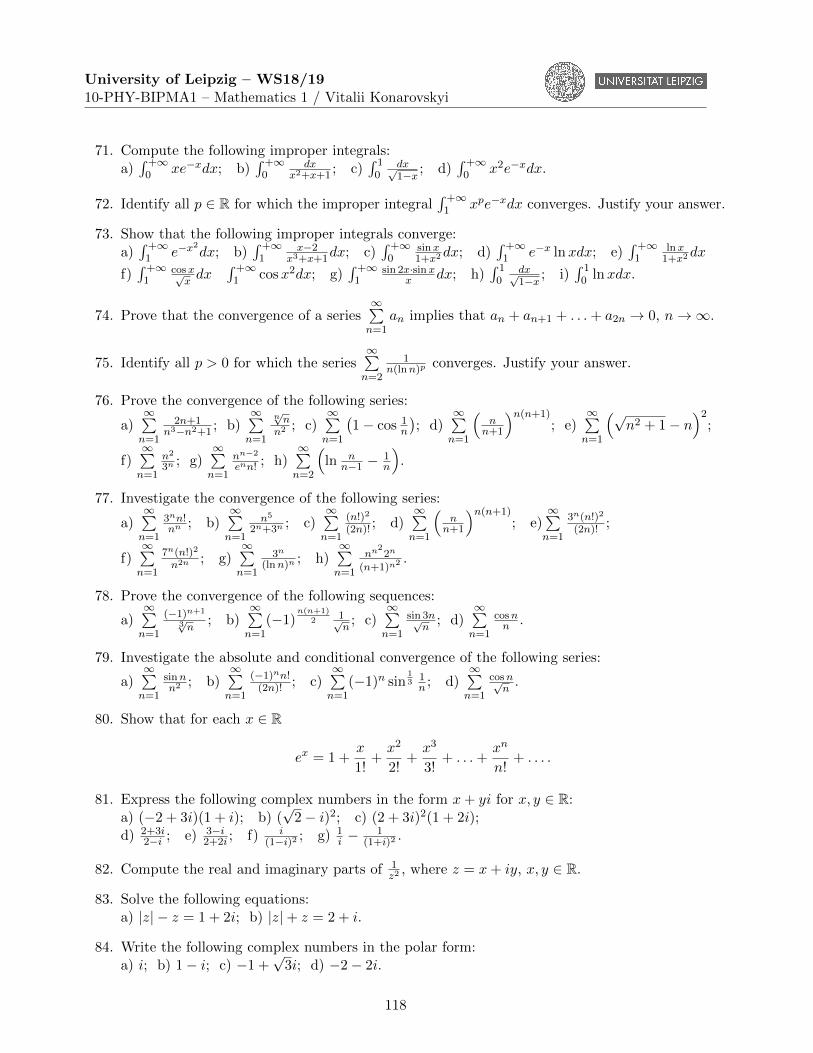
University of Leipzig – WS18/1910-PHY-BIPMA1 – Mathematics 1 / Vitalii Konarovskyi
71. Compute the following improper integrals:a)∫ +∞0 xe−xdx; b)
∫ +∞0
dxx2+x+1
; c)∫ 10
dx√1−x ; d)
∫ +∞0 x2e−xdx.
72. Identify all p ∈ R for which the improper integral∫ +∞1 xpe−xdx converges. Justify your answer.
73. Show that the following improper integrals converge:a)∫ +∞1 e−x
2dx; b)
∫ +∞1
x−2x3+x+1
dx; c)∫ +∞0
sinx1+x2
dx; d)∫ +∞1 e−x lnxdx; e)
∫ +∞1
lnx1+x2
dx
f)∫ +∞1
cosx√xdx
∫ +∞1 cosx2dx; g)
∫ +∞1
sin 2x·sinxx dx; h)
∫ 10
dx√1−x ; i)
∫ 10 lnxdx.
74. Prove that the convergence of a series∞∑n=1
an implies that an + an+1 + . . .+ a2n → 0, n→∞.
75. Identify all p > 0 for which the series∞∑n=2
1n(lnn)p converges. Justify your answer.
76. Prove the convergence of the following series:
a)∞∑n=1
2n+1n3−n2+1
; b)∞∑n=1
n√nn2 ; c)
∞∑n=1
(1− cos 1
n
); d)
∞∑n=1
(nn+1
)n(n+1); e)
∞∑n=1
(√n2 + 1− n
)2;
f)∞∑n=1
n2
3n ; g)∞∑n=1
nn−2
enn! ; h)∞∑n=2
(ln n
n−1 − 1n
).
77. Investigate the convergence of the following series:
a)∞∑n=1
3nn!nn ; b)
∞∑n=1
n5
2n+3n ; c)∞∑n=1
(n!)2
(2n)! ; d)∞∑n=1
(nn+1
)n(n+1); e)
∞∑n=1
3n(n!)2
(2n)! ;
f)∞∑n=1
7n(n!)2
n2n ; g)∞∑n=1
3n
(lnn)n ; h)∞∑n=1
nn22n
(n+1)n2.
78. Prove the convergence of the following sequences:
a)∞∑n=1
(−1)n+1
3√n ; b)∞∑n=1
(−1)n(n+1)
21√n
; c)∞∑n=1
sin 3n√n
; d)∞∑n=1
cosnn .
79. Investigate the absolute and conditional convergence of the following series:
a)∞∑n=1
sinnn2 ; b)
∞∑n=1
(−1)nn!(2n)! ; c)
∞∑n=1
(−1)n sin13
1n ; d)
∞∑n=1
cosn√n
.
80. Show that for each x ∈ R
ex = 1 +x
1!+x2
2!+x3
3!+ . . .+
xn
n!+ . . . .
81. Express the following complex numbers in the form x+ yi for x, y ∈ R:a) (−2 + 3i)(1 + i); b) (
√2− i)2; c) (2 + 3i)2(1 + 2i);
d) 2+3i2−i ; e) 3−i
2+2i ; f) i(1−i)2 ; g) 1
i − 1(1+i)2
.
82. Compute the real and imaginary parts of 1z2
, where z = x+ iy, x, y ∈ R.
83. Solve the following equations:a) |z| − z = 1 + 2i; b) |z|+ z = 2 + i.
84. Write the following complex numbers in the polar form:a) i; b) 1− i; c) −1 +
√3i; d) −2− 2i.
118
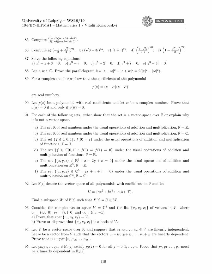
University of Leipzig – WS18/1910-PHY-BIPMA1 – Mathematics 1 / Vitalii Konarovskyi
85. Compute (1−√3i)(cos θ+i sin θ)
2(1−i)(cos θ−i sin θ) .
86. Compute a) (−12 +
√32 i)
21; b) (√
3− 3i)15; c) (1 + i)25; d)(1+√3i
1−i
)20; e)
(1−
√3−i2
)24.
87. Solve the following equations:a) z2 + z + 3 = 0; b) z3 − i = 0; c) z5 − 2 = 0; d) z4 + i = 0; e) z3 − 4i = 0.
88. Let z, w ∈ C. Prove the parallelogram law |z − w|2 + |z + w|2 = 2(|z|2 + |w|2).
89. For a complex number α show that the coefficients of the polynomial
p(z) = (z − α)(z − α)
are real numbers.
90. Let p(z) be a polynomial with real coefficients and let α be a complex number. Prove thatp(α) = 0 if and only if p(α) = 0.
91. For each of the following sets, either show that the set is a vector space over F or explain whyit is not a vector space.
a) The set R of real numbers under the usual operations of addition and multiplication, F = R.
b) The set R of real numbers under the usual operations of addition and multiplication, F = C.
c) The set {f ∈ C[0, 1] : f(0) = 2} under the usual operations of addition and multiplicationof functions, F = R.
d) The set {f ∈ C[0, 1] : f(0) = f(1) = 0} under the usual operations of addition andmultiplication of functions, F = R.
e) The set {(x, y, z) ∈ R3 : x − 2y + z = 0} under the usual operations of addition andmultiplication on R3, F = R.
f) The set {(x, y, z) ∈ C3 : 2x + z + i = 0} under the usual operations of addition andmultiplication on C3, F = C.
92. Let F[z] denote the vector space of all polynomials with coefficients in F and let
U = {az2 + bz5 : a, b ∈ F}.
Find a subspace W of F[z] such that F [z] = U ⊕W .
93. Consider the complex vector space V = C3 and the list {v1, v2, v3} of vectors in V , wherev1 = (i, 0, 0), v2 = (i, 1, 0) and v3 = (i, i,−1).a) Prove that span{v1, v2, v3} = V .b) Prove or disprove that {v1, v2, v3} is a basis of V .
94. Let V be a vector space over F, and suppose that v1, v2, . . . , vn ∈ V are linearly independent.Let w be a vector from V such that the vectors v1 +w, v2 +w, . . . , vn+w are linearly dependent.Prove that w ∈ span{v1, v2, . . . , vn}.
95. Let p0, p1, . . . , pn ∈ Fn[z] satisfy pj(2) = 0 for all j = 0, 1, . . . , n. Prove that p0, p1, . . . , pn mustbe a linearly dependent in Fn[z].
119
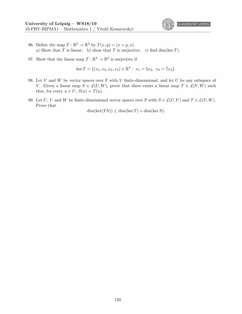
University of Leipzig – WS18/1910-PHY-BIPMA1 – Mathematics 1 / Vitalii Konarovskyi
96. Define the map T : R2 → R2 by T (x, y) = (x+ y, x).a) Show that T is linear; b) show that T is surjective; c) find dim(kerT ).
97. Show that the linear map T : R4 → R2 is surjective if
kerT = {(x1, x2, x3, x4) ∈ R4 : x1 = 5x2, x3 = 7x4}.
98. Let V and W be vector spaces over F with V finite-dimensional, and let U be any subspace ofV . Given a linear map S ∈ L(U,W ), prove that there exists a linear map T ∈ L(V,W ) suchthat, for every u ∈ U , S(u) = T (u).
99. Let U , V and W be finite-dimensional vector spaces over F with S ∈ L(U, V ) and T ∈ L(V,W ).Prove that
dim(ker(TS)) ≤ dim(kerT ) + dim(kerS).
120
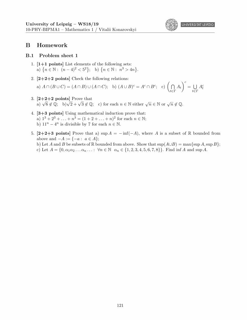
University of Leipzig – WS18/1910-PHY-BIPMA1 – Mathematics 1 / Vitalii Konarovskyi
B Homework
B.1 Problem sheet 1
1. [1+1 points] List elements of the following sets:a){n ∈ N : (n− 4)2 < 52
}; b)
{n ∈ N : n3 > 4n
}.
2. [2+2+2 points] Check the following relations:
a) A ∩ (B ∪ C) = (A ∩B) ∪ (A ∩ C); b) (A ∪B)c = Ac ∩Bc; c)
( ⋂t∈T
At
)c=⋃t∈T
Act
3. [2+2+2 points] Prove thata)√
6 6∈ Q; b)√
2 +√
3 6∈ Q; c) for each n ∈ N either√n ∈ N or
√n 6∈ Q.
4. [3+3 points] Using mathematical induction prove that:a) 13 + 23 + . . .+ n3 = (1 + 2 + . . .+ n)2 for each n ∈ N;b) 11n − 4n is divisible by 7 for each n ∈ N.
5. [2+2+3 points] Prove that a) supA = − inf(−A), where A is a subset of R bounded fromabove and −A := {−a : a ∈ A};b) Let A and B be subsets of R bounded from above. Show that sup(A∪B) = max{supA, supB};c) Let A = {0, α1α2 . . . αn . . . : ∀n ∈ N αn ∈ {1, 2, 3, 4, 5, 6, 7, 8}}. Find inf A and supA.
121
University of Leipzig – WS18/1910-PHY-BIPMA1 – Mathematics 1 / Vitalii Konarovskyi
B.2 Problem sheet 2
1. [1+1+1 points] Using the definition of the limit show thata) lim
n→∞n−1n = 1; b) lim
n→∞n2 = +∞; c) lim
n→∞(−1)n doe not exist.
2. [3 points] Assume that an → a, n→∞, and bn → b, n→∞. Show that max{an, bn} → max{a, b},n→∞.
3. [2+2+2 points] Compute the following limits:
a) limn→∞
n3−2n2 cosn+n√n−3n3+1
; b) limn→∞
(√n2 + n−√n); c) lim
n→∞n√n22n + 3n.
4. [3 points] Let (an)n≥1 be a bounded sequence and bn → 0, n ≥ ∞. Prove that anbn → 0,n→∞.
5. [3+3 points] Using the monotonicity compute the following limits:
a) limn→∞
n!
2n2; b) lim
n→∞
√2 +
√2 + . . .+
√2 +√
2︸ ︷︷ ︸n square roots
.
6. [2 points] Show that limn→∞
n ln(1 + 1
n
)= 1.
7. [2 points] Identify the set of subsequential limits of the sequence(sin 2πn
3
)n≥1.
122
University of Leipzig – WS18/1910-PHY-BIPMA1 – Mathematics 1 / Vitalii Konarovskyi
B.3 Problem sheet 3
1. [1+1+1 points] For a sequence (an)n≥1 compute limn→∞
an and limn→∞
an, if for all n ≥ 1
a) an = 1 + 1n ; b) an = 1 + n sin nπ
2 ; c) an = (−1)nn + 1+(−1)n
2 .
2. [3 points] Show that a := limn→∞
an = limn→∞
infk≥n
ak, for the case a ∈ R.
(The equality also holds in the case a ∈ {−∞,+∞})
3. [2 points] Check that the sequence(an = sin 1
21+ sin 2
22+ . . .+ sinn
2n
)n≥1 is a Cauchy sequence.
4. [2+2+2 points] Find the domain and the range of the following functions:a) f(x) = 1
(x+1)2; b) f(x) =
√1− x2; c) f(x) = ln(1 + x).
5. [2+2 points] Find the formulas for the following implicitly defined functions. What are theirdomains?a) y = f(x) is the solution to the equation x3y + 2y = 5;b) y = f(x) is the largest solution to the equation y2 = 3x2 − 2xy.
123
University of Leipzig – WS18/1910-PHY-BIPMA1 – Mathematics 1 / Vitalii Konarovskyi
B.4 Problem sheet 4
1. [1+1+1 points] Let f : X → Y . Check thata) f(A1 ∩A2) ⊂ (f(A1) ∩ f(A2)) for A1 ⊂ X, A2 ⊂ X;b) f−1(B1 ∪B2) = f−1(B1) ∪ f−1(B2) for B1 ⊂ Y , B2 ⊂ Y ;c) f(f−1(B)) = B ∩ f(X) for B ⊂ Y .
2. [2 points] Show that the set of all limit points of the set A = {r ∈ [0, 1] : r is rational} coincideswith the interval [0, 1]. (Hint: Use Theorem 2.3)
3. [2 point] Prove that the limit of the function f(x) = cos 1x , x ∈ R \ {0}, does not exist at the
point a = 0.
4. [2+2 point] Using ε− δ definition, show thata) lim
x→4
√x = 2; b) lim
x→+∞lnxx = 0.
5. [2+2+2 points] Compute the following limits:
a) limx→0
1−cosxx2
; b) limx→+∞
x3−x sinx+x1−3x3+lnx
; c) limx→1
x2−xx2−3x+2
.
6. [2 points] Let a be a limit point of A ⊂ R and f, g : A→ R satisfy the following properties:1) f is bounded on A; 2) g(x)→ 0, x→ a. Show that lim
x→a(f(x) · g(x)) = 0.
(Hint: Use Squeeze theorem for functions)
7. [2+2+2 points] Compute the following limits:
a) limx→0−
x√1−cos2 x ; b) lim
x→0+
x√1−cos2 x ; c) lim
x→0+e−
1x .
124
University of Leipzig – WS18/1910-PHY-BIPMA1 – Mathematics 1 / Vitalii Konarovskyi
B.5 Problem sheet 5
1. [1+1 points] Let a, b be a real numbers, f(x) = x+ 1, x ≤ 0 and f(x) = ax+ b, x > 0. a) Forwhich a, b the function f is monotone on R? b) For which a, b the function f is continuous onR?
2. [1+1 points] Compute the following limits:
a) limx→0
(tanx− ex); b) limx→2
x2−3x+1x−sinπx .
3. [2 points] Let f(x) = bxc sinπx, x ∈ R. Prove that f is continuous on R and sketch its graph.(Hint: If x ∈ [k, k+ 1) for some k ∈ Z, then bxc = k and f(x) = k sinπx. Find f(k−) and f(k+) at the points k.)
4. [2 points] Prove that the function f(x) = sin 1x , x 6= 0, and f(0) = 0, is discontinuous at 0.
5. [2x6 points] Compute the following limits:
a) limx→0
arcsinxx ; b) lim
x→0(cosx)
1x2 ; c) lim
x→+∞x(ln(1 + x)− lnx); d) lim
x→0
(1+sin 2xcos 2x
) 1x ;
e) limx→0
7√cosx−13√1+x2−1
; f) limx→0
esin 2x−etan xx .
6. [2 points] Prove that the function P (x) = x3 + 7x2 − 1, x ∈ R, has at least one root, that is,there exists x0 ∈ R such that P (x0) = 0.
7. [3 points] Let f : [a, b] → R strictly increase on [a, b] and for each y0 ∈ [f(a), f(b)] there existx0 ∈ [a, b] such that f(x0) = y0. Prove that f is continuous on [a, b].
8. [2 points] Using the definition, show that the function f(x) =√x, x ∈ [1,+∞), is uniformly
continuous on [1,+∞).
125
University of Leipzig – WS18/1910-PHY-BIPMA1 – Mathematics 1 / Vitalii Konarovskyi
B.6 Problem sheet 6
1. [1+1+1 points] Express through f ′(a) the following limits:
a) limh→0
f(a+2h)−f(a)h ; b) lim
h→0
f(a+h)−f(a−h)h ; c) lim
n→∞n(f(n+1n a
)− f(a)
).
2. [2 points] Using the definition of derivative, check that (x|x|)′ = 2|x|, x ∈ R.
3. [3 points] For the function f(x) = |x2 − x|, x ∈ R, compute f ′(x) for each x ∈ R \ {0, 1}.Compute left and right derivatives at points 0 and 1.
4. [1+2 points] Let
f(x) =
{x2, x ≤ 1,
ax+ b, x > 1.
For which a, b ∈ R the function f :a) is continuous on R; b) is differentiable on R? Compute also f ′.
5. [2x3 points] Check whether the following functions are differentiable at 0. Justify your answer.
a) f(x) =
{cosx−1
x , x 6= 0,
0, x = 0;b)f(x) =
5√x2, x ∈ R; c) f(x) = | sinx|, x ∈ R.
6. [1x8 points] Compute derivatives of the following functions:
a) f(x) = x2 sinx; b) f(x) = e−x2
2 cosx; c) f(x) = x1+x2
; d) f(x) = ex+e−x
ex−e−x ;
e) f(x) = 2tan(x2−1); f) f(x) = sin(cos2(tan3 x)); g) f(x) = 3
√1+x3
1−x3 ;
h) f(x) = eax · a sin bx−b cos bx√a2+b2
, where a, b are some constants.
126
University of Leipzig – WS18/1910-PHY-BIPMA1 – Mathematics 1 / Vitalii Konarovskyi
B.7 Problem sheet 7
1. [1x6 points] Compute derivatives of the following functions:
a) f(x) = 14 ln x2−1
x2+1; b) f(x) = ln
(x+√x2 + 1
); c) f(x) = ln tan x
2 ;
d) f(x) = arcsin 1−x√2
; e) f(x) = arctan 1+x1−x ; f) f(x) = x
√x.
2. [2 points] Let a function f : (a, b) → R be differentiable on (a, b) and there exists L ∈ R suchthat |f ′(x)| ≤ L for all x ∈ (a, b). Show that f is uniformly continuous on (a, b).
3. [2 points] Prove the equality
3 arccosx− arccos(3x− 4x3) = π, x ∈[−1
2,1
2
].
(Hint: Compute derivatives of the left and right hand sides of the equality)
4. [3 points] Let functions f, g : (a, b)→ (0,+∞) be differentiable on (a, b) and for every x ∈ (a, b)f ′(x)f(x) = g′(x)
g(x) . Prove that there exists L > 0 such that f(x) = Lg(x) for all x ∈ (a, b).
(Hint: Consider the functions ln f and ln g)
5. [3 points] (Generalised Bernoulli inequality) For each α > 1, prove that (1 + x)α ≥ 1 + αx forall x > −1. Moreover, (1 + x)α = 1 + αx iff x = 0.
6. [2x4 points] Identify the intervals on which the following functions are monotone.
a) f(x) = 3x− x3, x ∈ R b)f(x) = 2x1+x2
, x ∈ R; c) f(x) = x2
2x , x ∈ R;
d) f(x) = x+√|1− x2|, x ∈ R.
127
University of Leipzig – WS18/1910-PHY-BIPMA1 – Mathematics 1 / Vitalii Konarovskyi
B.8 Problem sheet 8
1. [1x4 points] Using L’Hospital’s Rule, show that
a) limx→0
ln(1+x)sinx = 1; b)lim
x→e(lnx)α−(xe )
β
x−e = α−βe , where α, β are some real numbers;
c) limx→+∞
lnxxε = 0 for all ε > 0; d) lim
x→+0(ln(1 + x))x = 1.
2. [3x3 points] Using L’Hospital’s Rule, compute the following limits:
a) limx→0
ex−esin xx−sinx ; b) lim
x→0+
(ln(1+x)
x
) 1x; c) lim
x→0
(1+x)1x−e
x .
3. [2x3 points] Compute the n-th derivative of the following functions:a) f(x) = 2x−1, x ∈ R; b) f(x) =
√2x− 1, x > 1
2 ; c) (x2ex)(n), x ∈ R.
(Hint: Use the Leibniz Formula in c))
4. [3 points] Write Taylor’s expansion of the function e2x−x2, x ∈ R at the point x0 = 0 up to the
term with x5.
5. [2x2 points] Use Taylor’s formula to compute the limits
a) limx→0
cosx−e−x2
2
x4; b) lim
x→0
ex sinx−x(1+x)x3
.
128
University of Leipzig – WS18/1910-PHY-BIPMA1 – Mathematics 1 / Vitalii Konarovskyi
B.9 Problem sheet 9
1. [1x3 points] Find points of local extrema of the following functions:a) f(x) = x2ex, x ∈ R; b) f(x) = x+ 1
x , x > 0; c) f(x) = |x|e−x2 , x ∈ R.
2. [1x3 points] Identify intervals on which the following functions are convex or concave:a) f(x) = 1
x , x > 0; b) f(x) = arctanx, x ∈ R.
3. [3 points](Young’s inequality) Let p > 1, q > 1 and 1p + 1
q = 1.
Prove that xy ≤ xp
p + yq
q for all x, y ∈ (0,+∞).
(Hint: Consider the function f(x) = − lnx, x > 0, and use its convexity on (0,+∞))
4. [2x9 points] Compute the following indefinite integrals:
a)∫
dxx lnx , x > 0; b)
∫ (2x+1)dx3√1+x+x2
, x ∈ R; c)∫ √
tanxcos2 x
dx, x ∈(0, π2
);
d)∫
dxcosx , x ∈
(−π
2 ,π2
); e)
∫cos2 x sin3 xdx, x ∈ R; f)
∫dx
x2+x+1, x ∈ R;
g)∫x2 sinxdx, x ∈ R; h)
∫(lnx)2dx, x > 0; i)
∫e2x cosxdx, x ∈ R.
129
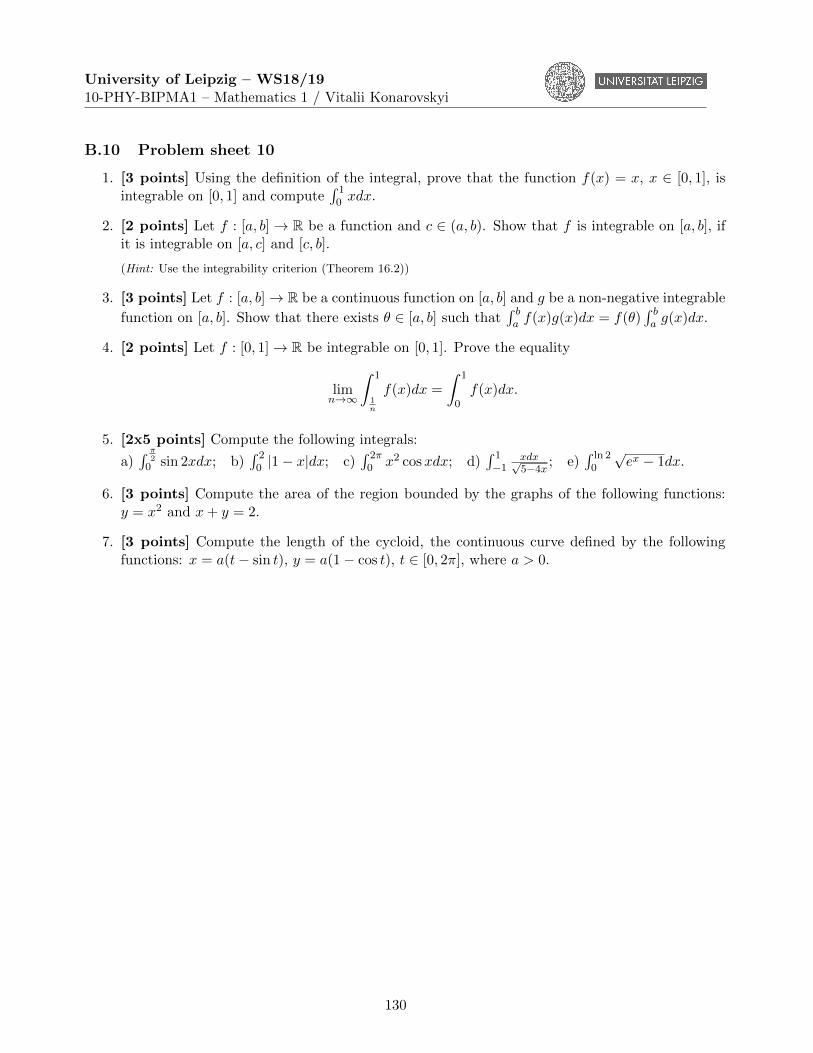
University of Leipzig – WS18/1910-PHY-BIPMA1 – Mathematics 1 / Vitalii Konarovskyi
B.10 Problem sheet 10
1. [3 points] Using the definition of the integral, prove that the function f(x) = x, x ∈ [0, 1], isintegrable on [0, 1] and compute
∫ 10 xdx.
2. [2 points] Let f : [a, b]→ R be a function and c ∈ (a, b). Show that f is integrable on [a, b], ifit is integrable on [a, c] and [c, b].
(Hint: Use the integrability criterion (Theorem 16.2))
3. [3 points] Let f : [a, b]→ R be a continuous function on [a, b] and g be a non-negative integrable
function on [a, b]. Show that there exists θ ∈ [a, b] such that∫ ba f(x)g(x)dx = f(θ)
∫ ba g(x)dx.
4. [2 points] Let f : [0, 1]→ R be integrable on [0, 1]. Prove the equality
limn→∞
∫ 1
1n
f(x)dx =
∫ 1
0f(x)dx.
5. [2x5 points] Compute the following integrals:
a)∫ π
20 sin 2xdx; b)
∫ 20 |1− x|dx; c)
∫ 2π0 x2 cosxdx; d)
∫ 1−1
xdx√5−4x ; e)
∫ ln 20
√ex − 1dx.
6. [3 points] Compute the area of the region bounded by the graphs of the following functions:y = x2 and x+ y = 2.
7. [3 points] Compute the length of the cycloid, the continuous curve defined by the followingfunctions: x = a(t− sin t), y = a(1− cos t), t ∈ [0, 2π], where a > 0.
130
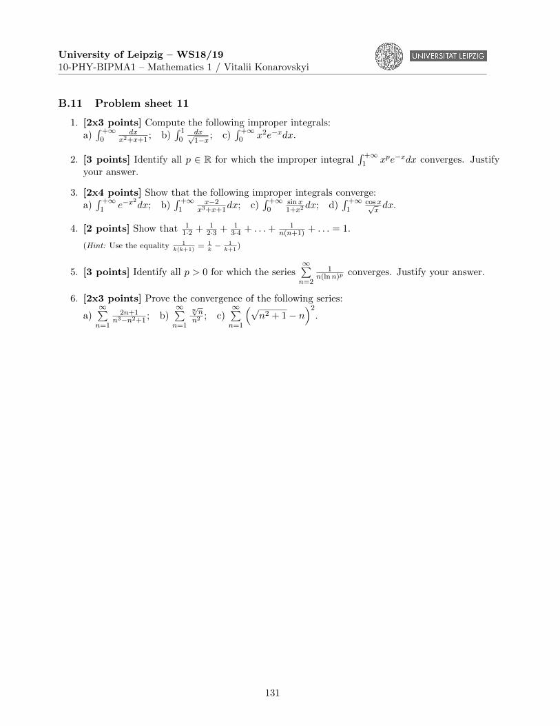
University of Leipzig – WS18/1910-PHY-BIPMA1 – Mathematics 1 / Vitalii Konarovskyi
B.11 Problem sheet 11
1. [2x3 points] Compute the following improper integrals:a)∫ +∞0
dxx2+x+1
; b)∫ 10
dx√1−x ; c)
∫ +∞0 x2e−xdx.
2. [3 points] Identify all p ∈ R for which the improper integral∫ +∞1 xpe−xdx converges. Justify
your answer.
3. [2x4 points] Show that the following improper integrals converge:a)∫ +∞1 e−x
2dx; b)
∫ +∞1
x−2x3+x+1
dx; c)∫ +∞0
sinx1+x2
dx; d)∫ +∞1
cosx√xdx.
4. [2 points] Show that 11·2 + 1
2·3 + 13·4 + . . .+ 1
n(n+1) + . . . = 1.
(Hint: Use the equality 1k(k+1)
= 1k− 1
k+1)
5. [3 points] Identify all p > 0 for which the series∞∑n=2
1n(lnn)p converges. Justify your answer.
6. [2x3 points] Prove the convergence of the following series:
a)∞∑n=1
2n+1n3−n2+1
; b)∞∑n=1
n√nn2 ; c)
∞∑n=1
(√n2 + 1− n
)2.
131
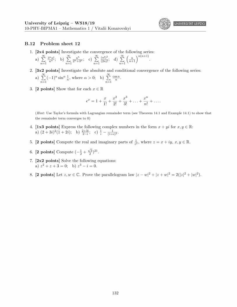
University of Leipzig – WS18/1910-PHY-BIPMA1 – Mathematics 1 / Vitalii Konarovskyi
B.12 Problem sheet 12
1. [2x4 points] Investigate the convergence of the following series:
a)∞∑n=1
3nn!nn ; b)
∞∑n=1
n5
2n+3n ; c)∞∑n=1
(n!)2
(2n)! ; d)∞∑n=1
(nn+1
)n(n+1).
2. [3x2 points] Investigate the absolute and conditional convergence of the following series:
a)∞∑n=1
(−1)n sinα 1n , where α > 0; b)
∞∑n=1
cosnn .
3. [2 points] Show that for each x ∈ R
ex = 1 +x
1!+x2
2!+x3
3!+ . . .+
xn
n!+ . . . .
(Hint: Use Taylor’s formula with Lagrangian remainder term (see Theorem 14.1 and Example 14.1) to show that
the remainder term converges to 0)
4. [1x3 points] Express the following complex numbers in the form x+ yi for x, y ∈ R:a) (2 + 3i)2(1 + 2i); b) 2+3i
2−i ; c) 1i − 1
(1+i)2.
5. [2 points] Compute the real and imaginary parts of 1z2
, where z = x+ iy, x, y ∈ R.
6. [2 points] Compute (−12 +
√32 )21.
7. [2x2 points] Solve the following equations:a) z2 + z + 3 = 0; b) z3 − i = 0.
8. [2 points] Let z, w ∈ C. Prove the parallelogram law |z − w|2 + |z + w|2 = 2(|z|2 + |w|2).
132
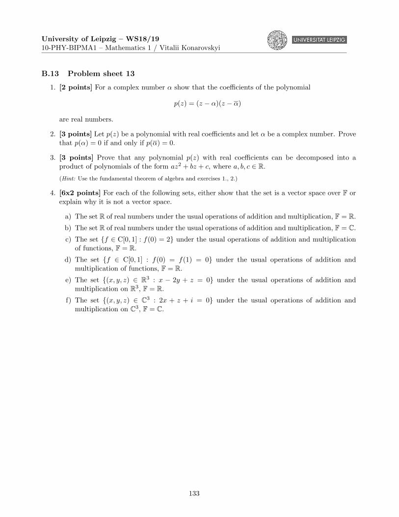
University of Leipzig – WS18/1910-PHY-BIPMA1 – Mathematics 1 / Vitalii Konarovskyi
B.13 Problem sheet 13
1. [2 points] For a complex number α show that the coefficients of the polynomial
p(z) = (z − α)(z − α)
are real numbers.
2. [3 points] Let p(z) be a polynomial with real coefficients and let α be a complex number. Provethat p(α) = 0 if and only if p(α) = 0.
3. [3 points] Prove that any polynomial p(z) with real coefficients can be decomposed into aproduct of polynomials of the form az2 + bz + c, where a, b, c ∈ R.
(Hint: Use the fundamental theorem of algebra and exercises 1., 2.)
4. [6x2 points] For each of the following sets, either show that the set is a vector space over F orexplain why it is not a vector space.
a) The set R of real numbers under the usual operations of addition and multiplication, F = R.
b) The set R of real numbers under the usual operations of addition and multiplication, F = C.
c) The set {f ∈ C[0, 1] : f(0) = 2} under the usual operations of addition and multiplicationof functions, F = R.
d) The set {f ∈ C[0, 1] : f(0) = f(1) = 0} under the usual operations of addition andmultiplication of functions, F = R.
e) The set {(x, y, z) ∈ R3 : x − 2y + z = 0} under the usual operations of addition andmultiplication on R3, F = R.
f) The set {(x, y, z) ∈ C3 : 2x + z + i = 0} under the usual operations of addition andmultiplication on C3, F = C.
133
University of Leipzig – WS18/1910-PHY-BIPMA1 – Mathematics 1 / Vitalii Konarovskyi
B.14 Problem sheet 14
1. [1 point] Let V be a vector space over F. Then, given a ∈ F and v ∈ V such that av = 0, provethat either a = 0 or v = 0.
2. [2x3 points] Prove or give a counterexample to the following claim:
1) Let V be a vector space over F and suppose that W1, W2 and W3 are subspaces of V suchthat W1 +W3 = W2 +W3. Then W1 = W2.
2) Let V be a vector space over F and suppose that W1, W2 and W3 are subspaces of V suchthat W1 ⊕W3 = W2 ⊕W3. Then W1 = W2.
3. [2 points] Let F[z] denote the vector space of all polynomials with coefficients in F and let
U = {az2 + bz5 : a, b ∈ F}.
Find a subspace W of F[z] such that F [z] = U ⊕W .
4. [2x2 points] Consider the complex vector space V = C3 and the list {v1, v2, v3} of vectors inV , where v1 = (i, 0, 0), v2 = (i, 1, 0) and v3 = (i, i,−1).a) Prove that span{v1, v2, v3} = V .b) Prove or disprove that {v1, v2, v3} is a basis of V .
5. [2 points] Let V be a vector space over F, and suppose that v1, v2, . . . , vn ∈ V are linearlyindependent. Let w be a vector from V such that the vectors v1 + w, v2 + w, . . . , vn + w arelinearly dependent. Prove that w ∈ span{v1, v2, . . . , vn}.
6. [3 points] Let p0, p1, . . . , pn ∈ Fn[z] satisfy pj(2) = 0 for all j = 0, 1, . . . , n. Prove thatp0, p1, . . . , pn must be a linearly dependent in Fn[z].
7. [3x1 points] Define the map T : R2 → R2 by T (x, y) = (x+ y, x).a) Show that T is linear; b) show that T is surjective; c) find dim(kerT ).
8. [3 points] Show that the linear map T : R4 → R2 is surjective if
kerT = {(x1, x2, x3, x4) ∈ R4 : x1 = 5x2, x3 = 7x4}.
9. [3 points] Let V and W be vector spaces over F with V finite-dimensional, and let U beany subspace of V . Given a linear map S ∈ L(U,W ), prove that there exists a linear mapT ∈ L(V,W ) such that, for every u ∈ U , S(u) = T (u).
10. [3 points] Let V and W be vector spaces over F with V finite-dimensional. Given T ∈ L(V,W ),prove that there is a subspace U of V such that U ∩ kerT = {0} and rangeT = {T (u) : u ∈ U}.
11. [3 points] Let U , V and W be finite-dimensional vector spaces over F with S ∈ L(U, V ) andT ∈ L(V,W ). Prove that
dim(ker(TS)) ≤ dim(kerT ) + dim(kerS).
134
University of Leipzig – WS18/1910-PHY-BIPMA1 – Mathematics 1 / Vitalii Konarovskyi
C Exam
1. Show that for every n ∈ N
12 + 22 + 32 + . . .+ n2 =n(n+ 1)(2n+ 1)
6.
2. Let (an)n≥1 be a sequence such that ann → 0, n→∞. Prove that max{a1,a2,...,an}
n → 0, n→∞.
3. Is the function
f(x) =
{1−cosxsinx , x 6= 0,
0, x = 0,x ∈ (−π, π),
continuous on (−π, π)? Is f differentiable on (−π, π)? Compute the derivative of f at each pointwhere it exists.
4. Compute the limit limx→0
(1 + arcsin2 x
) 1tan2 x .
5. Find points of local maximum and minimum of the function f(x) = x2(x− 5)3, x ∈ R.
6. Compute the length of continuous curve defined by the function y = x32 , x ∈ [0, 4].
7. Compute the improper integral∫ +∞2
lnxx2dx.
8. Investigate the absolute and conditional convergence of the series∞∑n=1
(−1)n ln(
1 + 1√n
).
9. Compute(1+√3i
1−i
)12.
10. Show that there does not exist any linear map T : R5 → R2 with
kerT = {(x1, x2, x3, x4, x5) : x1 = x2, x3 = x4 = −x5}.
11. Write the Taylor formulas with the Peano remainder term and the Lagrangian remainder term(indicate also conditions on the function under which the Taylor formulas are true).
12. Give definitions of linearly independent set of vectors, linear span and basis.
135
University of Leipzig – WS18/1910-PHY-BIPMA1 – Mathematics 1 / Vitalii Konarovskyi
D Exam Solutions
1. Show that for every n ∈ N
12 + 22 + 32 + . . .+ n2 =n(n+ 1)(2n+ 1)
6. (49)
Solution. To prove equality (49), we use the mathematical induction. For n = 1 we have12 = 1·2·3
6 . We assume that (49) is true for n ∈ N and check it for n+ 1. So,
12 + 22 + 32 + . . .+ n2 + (n+ 1)2 =n(n+ 1)(2n+ 1)
6+ (n+ 1)2
=n(n+ 1)(2n+ 1) + 6(n+ 1)2
6=
(n+ 1) (n(2n+ 1) + 6(n+ 1))
6.
In order to finish the proof, we have to check that n(2n+1)+6(n+1) = (n+2)(2(n+1)+1). Forthis, we compute n(2n+1)+6(n+1) = 2n2+7n+6 and (n+2)(2(n+1)+1) = (n+2)(2n+3) =2n2 + 7n+ 6.
2. Let (an)n≥1 be a sequence such that ann → 0, n→∞. Prove that max{a1,a2,...,an}
n → 0, n→∞.
Solution. Let ε > 0 be fixed. Since ann → 0, n → ∞, there exists N1 ∈ N such that for all
n ≥ N1
∣∣ann − 0
∣∣ = |an|n < ε. We next choose N2 ∈ N such that |ak|N2
< ε for all k = 1, . . . , N1.Thus, taking N := max{N1, N2}, we can estimate for every n ≥ N and k = 1, . . . , n
|ak|n≤ |ak|
N2< ε, if k ≤ N1,
and|ak|n≤ |ak|
k< ε, if N1 < k ≤ n.
Hence, we have ∣∣∣∣max{a1, a2, . . . , an}n
∣∣∣∣ ≤ max{|a1|, |a2|, . . . , |an|}n
< ε.
This implies that max{a1,a2,...,an}n → 0, n→∞.
3. Is the function
f(x) =
{1−cosxsinx , x 6= 0,
0, x = 0,x ∈ (−π, π),
continuous on (−π, π)? Is f differentiable on (−π, π)? Compute the derivative of f at each pointwhere it exists.
Solution. Since sin and cos are continuous functions and sinx 6= 0 for all x ∈ (−π, π) \ {0}, thefunction f is continuous at each point of (−π, π) \ {0}. To check the continuity of f at 0, wecompute
limx→0
f(x) = limx→0
1− cosx
sinx= lim
x→0
x2(1− cosx)
x2 sinx
= limx→0
x · limx→0
x
sinx· limx→0
1− cosx
x2= 0 · 1 · 1
2= 0 = f(0).
136
University of Leipzig – WS18/1910-PHY-BIPMA1 – Mathematics 1 / Vitalii Konarovskyi
Hence, the function f is continuous at 0 and, consequently, it is continuous on (−π, π).
Similarly, f is differentiable at each point of (−π, π) \ {0} because sin and cos are differentiableand sinx 6= 0 for all x ∈ (−π, π) \ {0}. Moreover, for every x ∈ (−π, π) \ {0}
f ′(x) =
(1− cosx
sinx
)′=
(1− cosx)′ sinx− (1− cosx)(sinx)′
sin2 x
=sin2 x− (1− cosx) cosx
sin2 x=
sin2 x+ cos2 x− cosx
sin2 x=
1− cosx
sin2 x.
We next compute
f ′(0) = limx→0
f(x)− f(0)
x− 0= lim
x→0
1− cosx
x sinx= lim
x→0
x(1− cosx)
x2 sinx
= limx→0
x
sinx· limx→0
1− cosx
x2=
1
2.
Hence the function f is differentiable on (−π, π) and
f ′(x) =
{1−cosxsin2 x
, x 6= 0,12 , x = 0,
x ∈ (−π, π),
4. Compute the limit limx→0
(1 + arcsin2 x
) 1tan2 x .
Solution.
limx→0
(1 + arcsin2 x
) 1tan2 x = lim
x→0eln(1+arcsin2 x)
1tan2 x
= limx→0
eln(1+arcsin2 x)
tan2 x
=e
limx→0
ln(1 + arcsin2 x
)tan2 x
,
by the continuity of the exponential function. So, we compute
limx→0
ln(1 + arcsin2 x
)tan2 x
= limx→0
arcsin2 x · ln(1 + arcsin2 x
)arcsin2 x · tan2 x
= limx→0
ln(1 + arcsin2 x
)arcsin2 x
· limx→0
arcsin2 x
tan2 x
= 1 · limx→0
x2 · arcsin2 x
x2 · tan2 x= lim
x→0
arcsin2 x
x2· limx→0
x2
tan2 x
=
(limx→0
arcsinx
x
)2
·(
limx→0
x
tanx
)2= 1.
Hence, limx→0
(1 + arcsin2 x
) 1tan2 x = e1 = e.
5. Find points of local maximum and minimum of the function f(x) = x2(x− 5)3, x ∈ R.
Solution. We first compute critical points of f :
f ′(x) =(x2(x− 5)3
)′=(x2)′
(x− 5)3 + x2((x− 5)3
)′= 2x(x− 5)3 + 3x2(x− 5)2
= x(x− 5)2 (2(x− 5) + 3x) = x(x− 5)2(5x− 10) = 0.
137
University of Leipzig – WS18/1910-PHY-BIPMA1 – Mathematics 1 / Vitalii Konarovskyi
Hence, the points x = 0, x = 2, x = 5 are critical.
The point 0 is a point of strict local maximum because the derivative changes its sign from “+”to “–”, passing through 0.
The point 2 is a point of strict local minimum because the derivative changes its sign from “–”to “+”, passing through 2.
The point 5 is not a point of local extrema because the derivative stays positive, passingthrough 5.
6. Compute the length of continuous curve defined by the function y = x32 , x ∈ [0, 4].
Solution. The length of the curve Γ defined by the function y = x32 , x ∈ [0, 4], can be computed
by the formula
l(Γ) =
∫ 4
0
√1 +
((x
32
)′)2
dx =
∫ 4
0
√1 +
(3
2x
12
)2
dx =
∫ 4
0
√1 +
9
4xdx =
∣∣∣∣∣∣y = 1 + 9
4x,x = 4
9(y − 1),dx = 4
9dy
∣∣∣∣∣∣=
4
9
∫ 10
1y
12dy =
4
9· y
12+1
12 + 1
∣∣∣∣∣10
1
=8
27· y 3
2
∣∣∣∣101
=8
27(10√
10− 1).
7. Compute the improper integral∫ +∞2
lnxx2dx.
Solution. First we change the variable and then use the integration by parts formula:
∫ +∞
2
lnx
x2dx =
∣∣∣∣∣∣y = lnx,x = ey,dx = eydy
∣∣∣∣∣∣ =
∫ +∞
ln 2
yey
e2ydy =
∫ +∞
ln 2ye−ydy = −
∫ +∞
ln 2yde−y
= −ye−y∣∣∣∣+∞ln 2
+
∫ +∞
ln 2e−ydy = ln 2 · e− ln 2 − e−y
∣∣∣∣+∞ln 2
=ln 2
2+ e− ln 2 =
1 + ln 2
2.
Another way of the computation without change of variable:∫ +∞
2
lnx
x2dx = −
∫ +∞
2lnxd
1
x= − lnx
1
x
∣∣∣∣+∞2
+
∫ +∞
2
1
xd lnx =
ln 2
2+
∫ +∞
2
1
x2dx
=ln 2
2− 1
x
∣∣∣∣+∞2
=1 + ln 2
2
8. Investigate the absolute and conditional convergence of the series∞∑n=1
(−1)n ln(
1 + 1√n
).
Solution. The series∞∑n=1
∣∣∣∣(−1)n ln
(1 +
1√n
)∣∣∣∣ =
∞∑n=1
ln
(1 +
1√n
)
diverges because ln(
1 + 1√n
)∼ 1√
n, n→∞, and
∞∑n=1
1√n
diverges.
138
University of Leipzig – WS18/1910-PHY-BIPMA1 – Mathematics 1 / Vitalii Konarovskyi
Since the sequence ln(
1 + 1√n
), n ≥ 1, is monotone and converges to 0, the series
∞∑n=1
(−1)n ln
(1 +
1√n
)converges, according to Leibniz’s test. This implies the conditional convergence of the series.
9. Compute(1+√3i
1−i
)12.
Solution. We first write the numbers 1 +√
3i and 1 − i in the polar form. We compute the
absolute volume r and the argument θ of 1 +√
3i. So, r =√
12 + (√
3)2 = 2 and cos θ = 12 ,
sin θ =√32 . Thus, θ = π
3 . So, we obtain
1 +√
3i = 2(
cosπ
3+ i sin
π
3
).
Similarly,
1− i =√
2(
cos(−π
4
)+ i sin
(−π
4
)).
Hence(1 +√
3i
1− i
)12
=
(2(cos π3 + i sin π
3
)√
2(cos(−π
4
)+ i sin
(−π
4
)))12
= 26(
cos(π
3+π
4
)+ i sin
(π3
+π
4
))12= 64
(cos
7π
12+ i sin
7π
12
)12
= 64
(cos
12 · 7π12
+ i sin12 · 7π
12
)= −64.
10. Show that there does not exist any linear map T : R5 → R2 with
kerT = {(x1, x2, x3, x4, x5) : x1 = x2, x3 = x4 = −x5}. (50)
Solution. We assume that there exists a map T : R5 → R2 with the kernel given by (50). Wefirst note that
kerT = {(x1, x2, x3, x4, x5) : x1 = x2, x3 = x4 = −x5} = {(a, a, b, b,−b) : a, b ∈ R}.
Thus, the vectors v1 = (1, 1, 0, 0, 0) and v2 = (0, 0, 1, 1,−1) form a basis of kerT , since they arelinearly independent and span kerT . Hence, dim(kerT ) = 2. Since 5 = dim(R5) = dim(kerT ) +dim(rangeT ) = 2+dim(rangeT ), we have that dim(rangeT ) = 3. But that is impossible becauserangeT ⊂ R2 and dim(R2) = 2.
139
University of Leipzig – WS18/1910-PHY-BIPMA1 – Mathematics 1 / Vitalii Konarovskyi
E Retake
1. For which n ∈ N the following inequality holds?
3n > 5n+ 2.
2. Compute the following limit
limn→∞
n√n55n + n3n.
3. Show that a sequence (an)n≥1 of real numbers is a Cauchy sequence if and only ifsup
n≥k,m≥k|an − am| → 0, k → +∞.
4. For which a ∈ R the following function f is differentiable on R?
f(x) =
{sinxex−1 , x 6= 0,
a, x = 0,x ∈ R.
Compute the derivative of f .
5. Prove that the function f(x) = xx is increasing on(1e ,∞
). Is it convex on
(1e ,∞
)?
6. Compute the area of the region bounded by the graphs of the following functions 2x = y2 and2y = x2.
7. Compute the improper integral∫∞0 |x− 1|e−xdx.
8. Does the following series converges?
∞∑n=1
1
n(ln2 n+ 1
) .9. Write the following complex numbers in algebraic form: i
(1−i)2 , (1−√
3i)15.
10. Let R4[z] denotes the vector space of all polynomials of degree at most 4 with coefficients in Rand let the linear operator T : R4[z] → R4[z] is defined as follows (Tp)(z) = p′′(z) (Tp is thesecond order derivative of polynomial p). Identify kerT and rangeT . Find a subspace W ofR4[z] such that kerT ⊕W = R4[z].
11. Formulate the Fermat theorem and the Lagrange (mean value) theorem.
12. Give the definition of subsequential limit of a sequence and the definitions of upper and lowerlimits.
140
University of Leipzig – WS18/1910-PHY-BIPMA1 – Mathematics 1 / Vitalii Konarovskyi
F Retake Solutions
1. For which n ∈ N the following inequality holds?
3n > 5n+ 2. (51)
Solution. We first we note that inequality (51) is not true for n = 1 (31 < 5 · 1 + 2) and n = 2(32 < 5 · 2 + 2). If n = 3, then the inequality holds because 33 = 27 > 5 · 3 + 2 = 17. In order toshow that inequality (51) is true for all n ≥ 3, we will use the mathematical induction. Let usassume that (51) holds for n = k for some k ≥ 3, i.e. 3k > 5k + 2, and prove it for n = k + 1.So, 3n+1 = 3n · 3 > (5k + 2) · 3 = 15k + 6 = 5(k + 1) + 2 + 10k − 1 > 5(k + 1) + 2. Hence, theinequality 3n > 5n+ 2 is true for all n ≥ 3.
2. Compute the following limit
limn→∞
n√n55n + n3n.
Solution. In order to compute the limit we will use the squeeze theorem. For this, we estimate
5(n√n)5
=n√n55n <
n√n55n + n3n <
n√n55n + n55n = 5
n√
2n5 = 5n√
2(n√n)5.
Since limn→∞ 5 ( n√n)
5= 5 · 15 = 5 and limn→∞ 5 n
√2 ( n√n)
5= 5 limn→∞
n√
2 · limn→∞ ( n√n)
5=
5 · 1 · 15 = 5, the squeeze theorem implies that
limn→∞
n√n55n + n3n = 5.
3. Show that a sequence (an)n≥1 of real numbers is a Cauchy sequence if and only ifsup
n≥k,m≥k|an − am| → 0, k → +∞.
Solution. Let (an)n≥1 be a Cauchy sequence and let ε > 0 be fixed. By the definition of Cauchysequence, there exists a number N such that
∀n,m ≥ N |an − am| <ε
2.
Thus, supn≥k,m≥k
|an − am| ≤ ε2 < ε for all k ≥ N . This implies that sup
n≥k,m≥k|an − am| → 0,
k → +∞.
Next, we assume that supn≥k,m≥k
|an − am| → 0, k → +∞. Then, by the definition of the conver-
gence, we have that there exists a number N such that
∀k ≥ N supn≥k,m≥k
|an − am| < ε.
In particular, this yields that for all n,m ≥ N |an − am| < ε. So, (an)n≥1 is a Cauchy sequence.
4. For which a ∈ R the following function f is differentiable?
f(x) =
{sinxex−1 , x 6= 0,
a, x = 0,x ∈ R.
141
University of Leipzig – WS18/1910-PHY-BIPMA1 – Mathematics 1 / Vitalii Konarovskyi
Compute the derivative of f .
Solution. It is clear that the function f is differentiable on R\{0}. So, we have to check whetherf is differentiable at x = 0. For this we first find a for which f is continuous. Only for that athe function could be differentiable. We compute
limx→0
f(x) = limx→0
sinx
ex − 1= lim
x→0
x sinx
x(ex − 1)= lim
x→0
sinx
x· limx→0
x
ex − 1= 1.
So, only for a = 1 limx→0 f(x) = f(0). This implies that f is continuous on R for a = 1. Let uscheck that f is differentiable at x = 0 for a = 1.
We compute for a = 1
f ′(0) = limx→0
f(x)− f(0)
x− 0= lim
x→0
sinxex−1 − 1
x= lim
x→0
sinx− ex + 1
(ex − 1)x
= limx→0
6 x− x3
3! + o(x3)− 6 1− 6 x− x2
2! − o(x2)+ 6 1( 6 1 + x+ o(x)− 6 1)x
= limx→0
6 x2(− x
3! + o(x3)x2− 1
2! −o(x2)x2
)6 x2(
1 + o(x)x
) = − 1
2!= −1
2.
Consequently, f ′(0) = −12 for a = 1. If a 6= 1, then the function f is not differentiable at x = 0
because it is not continuous.
It remains to compute
f ′(x) =
(sinx
ex − 1
)′=
cosx (ex − 1)− ex sinx
(ex − 1)2, x 6= 0.
5. Prove that the function f(x) = xx is increasing on(1e ,∞
). Is it convex on
(1e ,∞
)?
Solution. In order to show that f is increasing, it is enough to show that its derivative is positive.So, we compute
f ′(x) = (xx)′ =(elnx
x)′
=(ex lnx
)′= ex lnx
(lnx+
x
x
)= xx (lnx+ 1) > 0
for x ∈(1e ,∞
). Hence the function f is strictly increasing on
(1e ,∞
). To check the convexity,
we compute the second derivative:
f ′′(x) = (xx (lnx+ 1))′ = (xx)′ (lnx+ 1) + xx (lnx+ 1)′ = xx (lnx+ 1)2 + xx1
x> 0
on(1e ,∞
). Thus, the function f is strictly convex on
(1e ,∞
).
6. Compute the area of the region bounded by the graphs of the following functions 2x = y2 and2y = x2.
Solution. We have to compute the region between two parabolas which intersect each other at
points x = 0 and x = 2 (the points of intersection can be found from the equation 2x =(x2
2
)2).
Thus, the area can be computed by the formula∫ 2
0
(√2x− x2
2
)dx =
√2
∫ 2
0x
12dx− 1
2
∫ 2
0x2dx =
√2
2
3x
32
∣∣∣20− 1
6x3∣∣∣20
=4
3.
142
University of Leipzig – WS18/1910-PHY-BIPMA1 – Mathematics 1 / Vitalii Konarovskyi
7. Compute the improper integral∫∞0 |x− 1|e−xdx.
Solution.∫ ∞0|x− 1|e−xdx =
∫ 1
0|x− 1|e−xdx+
∫ ∞1|x− 1|e−xdx = −
∫ 1
0(x− 1)e−xdx+
∫ ∞1
(x− 1)e−xdx.
Let us compute the indefinite integral∫(x− 1)e−xdx = −
∫(x− 1)de−x = −(x− 1)e−x +
∫e−xd(x− 1)
= −(x− 1)e−x +
∫e−xdx = −(x− 1)e−x − e−x + C = −xe−x + C.
By the fundamental theorem of calculus,∫ ∞0|x− 1|e−xdx = −
(−xe−x
) ∣∣∣10
+(−xe−x
) ∣∣∣∞1
= e−1 − 0 + 0 + e−1 = 2e−1 =2
e.
8. Does the following series converges?
∞∑n=1
1
n(ln2 n+ 1
) .Solution. Since the sequence 1
n(ln2 n+1)decreases, we can use the integral criterion. According
to that criterion, the convergence of the series∑∞
n=11
n(ln2 n+1)is equivalent to the convergence
of the improper integral∫ ∞1
dx
x(ln2 x+ 1
) =
∫ ∞1
d lnx
ln2 x+ 1
y=lnx=
∫ ∞0
dy
y2 + 1= arctan y
∣∣∣∞0
=π
2<∞.
Hence, the series∑∞
n=11
n(ln2 n+1)converges.
9. Write the following complex numbers in algebraic form: i(1−i)2 , (1−
√3i)15.
Solution.
i
(1− i)2 =i
1− 2i+ i2=
i
1− 2i− 1=
i
−2i= −1
2.
In order to compute (1−√
3i)15, we will use de Moivre’s formula. For this, we need to rewritethe complex number 1−
√3i in polar form. So, the absolute value r of 1−
√3i is given by the
formula r =
√12 +
(√3)2
= 2. The argument θ of 1 −√
3i can be found from the equalities
cos θ = 12 and sin θ =
√32 . Hence, θ = −π
3 . Consequently, we can compute
(1−√
3i)15 =(
2(
cos(−π
3
)+ i sin
(−π
3
)))15= 215
(cos
(−15π
3
)+ i sin
(−15π
3
))= 215 (cos(−5π) + i sin(−5π)) = −215.
143
University of Leipzig – WS18/1910-PHY-BIPMA1 – Mathematics 1 / Vitalii Konarovskyi
10. Let R4[z] denotes the vector space of all polynomials of degree at most 4 with coefficients in Rand let the linear operator T : R4[z] → R4[z] is defined as follows (Tp)(z) = p′′(z) (Tp is thesecond order derivative of polynomial p). Identify kerT and rangeT . Find a subspace W ofR4[z] such that kerT ⊕W = R4[z].
Solution. We take p ∈ Rn[z]. Then p can be written as p(z) = a4z4 + a3z
3 + a2z2 + a1z + a0,
where ai ∈ R, i = 0, . . . , 4. So, by the definition of T ,
(Tp)(z) = 12a4z2 + 6a3z + 2a2 ∈ R2[z]. (52)
This implies that Tp = 0 if and only if a2 = a3 = a4 = 0. Hence,
kerT = {p ∈ R4[z] : Tp = 0} = {p(z) = a1z + a0 : a0, a1 ∈ R} = R1[z].
Next, we compute
rangeT = {q ∈ R4[z] : ∃p ∈ R4[z] such that Tp = q} = R2[z].
Indeed, if q(z) = b2z2 + b1z + b0 ∈ R2[z], then for p(z) = b2
12z4 + b1
6 z3 + b1
2 z2 we trivially have
Tp = q. So, rangeT ⊃ R2[z]. Moreover, equality (52) implies rangeT ⊂ R2[z].
In order to find a vector subspace W of R4[z] such that kerT ⊕W = R4[z], we recall that itshould be a vector subspace such that kerT +W = R4[z] and kerT ∩W = {0}. We set
W ={q(z) = b4z
4 + b3z3 + b2z
2 : b2, b3, b4 ∈ R}.
It is easily to see that W is a vector subspace of R4[z] and kerT + W = R2[z] + W = R4[z].Moreover, only zero polynomial belongs to both kerT = R2[z] and W . Hence, kerT⊕W = R4[z].
144
University of Leipzig – WS18/1910-PHY-BIPMA1 – Mathematics 1 / Vitalii Konarovskyi
G Some Important Limits
G.1 Limits of sequences
• limn→∞
1nα = 0, α > 0; (Corollary 3.1)
• limn→∞
nb
an = 0, a ∈ R, |a| > 1, b ∈ R; (Theorem 3.3)
• limn→∞
lgnnα = 0, α > 0; (Exercise 3.6 c))
• limn→∞
n√n = 1; (Theorem 3.4)
• limn→∞
an
n! = 0, a > 0; (Example 4.2 for a = 10)
• limn→∞
(1 + 1
n
)n= e; (Section 4.2)
• limn→∞
n ln(1 + 1
n
)= 1. (Exercise 4.9)
G.2 Limits of functions
• limx→+∞
xb
ax = 0, a ∈ R, |a| > 1, b ∈ R; (Example 7.3 for b ∈ N and Exercise 7.6 for the general case)
• limx→+∞
lnxxα = 0, α > 0; (Exercise 7.2 for α = 1)
• limx→0
sinxx = 1; (Example 6.5)
• limx→0
tanxx = 1; (Example 7.8 a))
• limx→0
arcsinxx = 1; (Exercise 8.11 c))
• limx→0
arctanxx = 1; (Exercise 8.11 e))
• limx→0
1−cosxx2
= 12 ; (Exercise 7.8 d))
• limx→+∞
(1 + 1
x
)x= lim
x→0(1 + x)
1x = e; (Example 7.2)
• limx→0
ex−1x = 1; (A partial case of Theorem 8.7)
• limx→0
ax−1x = ln a, a > 0; (Theorem 8.7)
• limx→0
ln(1+x)x = 1; (A partial case of Theorem 8.6)
• limx→0
loga(1+x)x = loga e, a > 0, a 6= 1; (Theorem 8.6)
• limx→0
(1+x)α−1x = α, α ∈ R. (Theorem 8.8)
145
University of Leipzig – WS18/1910-PHY-BIPMA1 – Mathematics 1 / Vitalii Konarovskyi
G.3 Derivatives of Elementary Functions
• (xα)′ = αxα−1, x > 0, for α ∈ R; (Example 10.6)
• (xn)′ = mxm−1, x ∈ R \ {0}, for m ∈ Z; (Exercise 10.6)
• (xn)′ = nxn−1, x ∈ R, for n ∈ N; (Exercise 10.6)
• (ax)′ = ax ln a, x ∈ R, for a > 0; (Example 10.7)
• (ex)′ = ex, x ∈ R; (Example 10.7)
• (sinx)′ = cosx, x ∈ R; (Example 10.8)
• (cosx)′ = − sinx, x ∈ R; (Example 10.8)
• (tanx)′ = 1cos2 x
, x ∈ R \{π2 + πk : k ∈ Z
}; (Example 10.8)
• (cotx)′ = − 1sin2 x
, x ∈ R \ {πk : k ∈ Z}; (Example 10.8)
• (logα x)′ = 1x lnα , x > 0, for α > 0, α 6= 1; (Example 11.1)
• (lnx)′ = 1x , x > 0; (Example 11.1)
• (arcsinx)′ = 1√1−x2 , x ∈ (−1, 1); (Example 11.3)
• (arccosx)′ = − 1√1−x2 , x ∈ (−1, 1); (Exercise 11.3)
• (arctanx)′ = 11+x2
, x ∈ R; (Example 11.2)
• (arccotx)′ = − 11+x2
, x ∈ R; (Exercise 11.2)
• (sinhx)′ = coshx, x ∈ R; (Exercise 10.9)
• (coshx)′ = sinhx, x ∈ R; (Exercise 10.9)
• (tanhx)′ = 1cosh2 x
, x ∈ R; (Exercise 10.9)
• (cothx)′ = − 1sinh2 x
, x ∈ R \ {0}. (Exercise 10.9)
146
University of Leipzig – WS18/1910-PHY-BIPMA1 – Mathematics 1 / Vitalii Konarovskyi
G.4 Taylor’s Expansion of Elementary Functions
• ex = 1 + x+ x2
2! + . . .+ xn
n! + o(xn), x→ 0; (Example 13.5)
• ln(1 + x) = x− x2
2 + x3
3 − . . .+ (−1)n−1 xn
n + o(xn), x→ 0; (Example 13.6)
• (1 + x)α = 1 + αx+ α(α−1)x22! + . . .+ α(α−1)...(α−n+1)xn
n! + o(xn), x→ 0, α ∈ R; (Example 13.7)
• sinx = x− x3
3! + x5
5! − . . .+ (−1)n x2n+1
(2n+1)! + o(x2n+2), x→ 0; (Exercise 13.8)
• cosx = 1− x2
2! + x4
4! − . . .+ (−1)n x2n
(2n)! + o(x2n+1), x→ 0; (Exercise 13.8)
• sinhx = x+ x3
3! + x5
5! + . . .+ x2n+1
(2n+1)! + o(x2n+2), x→ 0; (Exercise 13.9)
• coshx = 1 + x2
2! + x4
4! + . . .+ x2n
(2n)! + o(x2n+1), x→ 0. (Exercise 13.9)
147
University of Leipzig – WS18/1910-PHY-BIPMA1 – Mathematics 1 / Vitalii Konarovskyi
G.5 Indefinite Integrals of Elementary Functions
•∫xαdx = xα+1
α+1 + C, x ∈ (0,+∞), for all α ∈ R \ {−1}; (Example 10.6)∫xndx = xn
n+1 + C, x ∈ R, for all n ∈ N ∪ {0}; (Exercise 10.6)
•∫
1xdx = ln |x|+ C on each interval (−∞, 0) and (0,+∞); (Example 11.1)
•∫axdx = ax
ln a + C, x ∈ R for all a > 0, a 6= 1; (Example 10.7)
•∫exdx = ex + C, x ∈ R; (Example 10.7)
•∫
cosxdx = sinx+ C, x ∈ R; (Example 10.8)
•∫
sinxdx = − cosx+ C, x ∈ R; (Example 10.8)
•∫
dxcos2 x
= tanx+ C on each interval(−π
2 + nπ, π2 + nπ), n ∈ Z; (Example 10.8)
•∫
dxsin2 x
= − cotx+ C on each interval (nπ, π + nπ), n ∈ Z; (Example 10.8)
•∫
dx1+x2
= arctanx+ C, x ∈ R; (Example 11.2)
•∫
dx√1−x2 = arcsinx+ C, x ∈ (−1, 1); (Example 11.3)
•∫
dxa2+x2
= 1a arctan x
a + C, x ∈ R, a 6= 0;
•∫
dxa2−x2 = 1
2a ln∣∣∣a+xa−x
∣∣∣+ C on (−∞,−a), (−a, a) and (a,+∞), a > 0;
•∫
dx√a2−x2 = arcsin x
a + C, x ∈ (−a, a), a > 0;
•∫
dx√x2−a2 = ln |x+
√x2 − a2|+ C on (−∞,−a) and (a,+∞), a > 0;
•∫
dx√x2+a2
= ln |x+√x2 + a2|+ C, x ∈ R, a 6= 0.
148