1

Lazy Learning – Nearest NeighborLantz Ch 3

Wk 2, Part 1

2

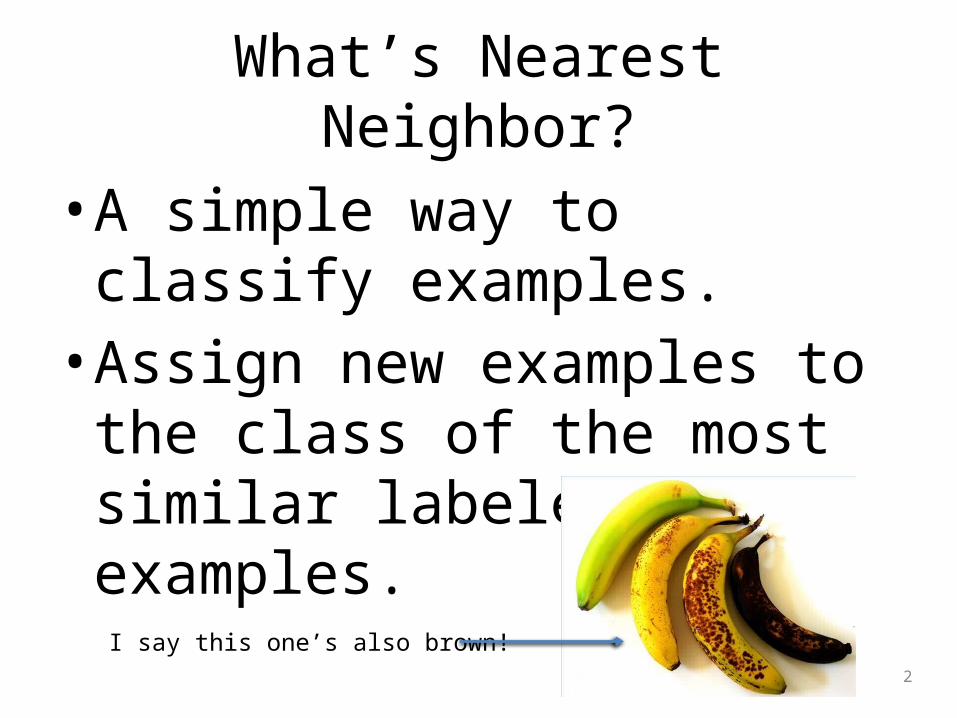
What’s Nearest Neighbor?

• A simple way to classify examples.• Assign new examples to the class

of the most similar labeled examples.

I say this one’s also brown!

3

The kNN algorithmStrengths Weaknesses

Simple and effective Does not produce a model, which limits the ability to find novel insights in relationships among features

Makes no assumptions about the underlying data distribution

Slow classification phase

Fast training phase Requires a large amount of memory

Nominal features and missing data require additional processing

kNN = “k-Nearest Neighbor”

4

kNN Training

• Begin with examples classified into several categories, labeled by a nominal variable.

• Need a training data set and a test dataset.• On the test dataset, kNN will identify k records

that are “nearest” in similarity.– You specify k in advance.– Each test example is assigned to the class of the

majority of the k nearest neighbors.

5

Lantz’s example

6

Need to calculate “distance”

• Euclidian –

• Manhattan – Add absolute values.

7

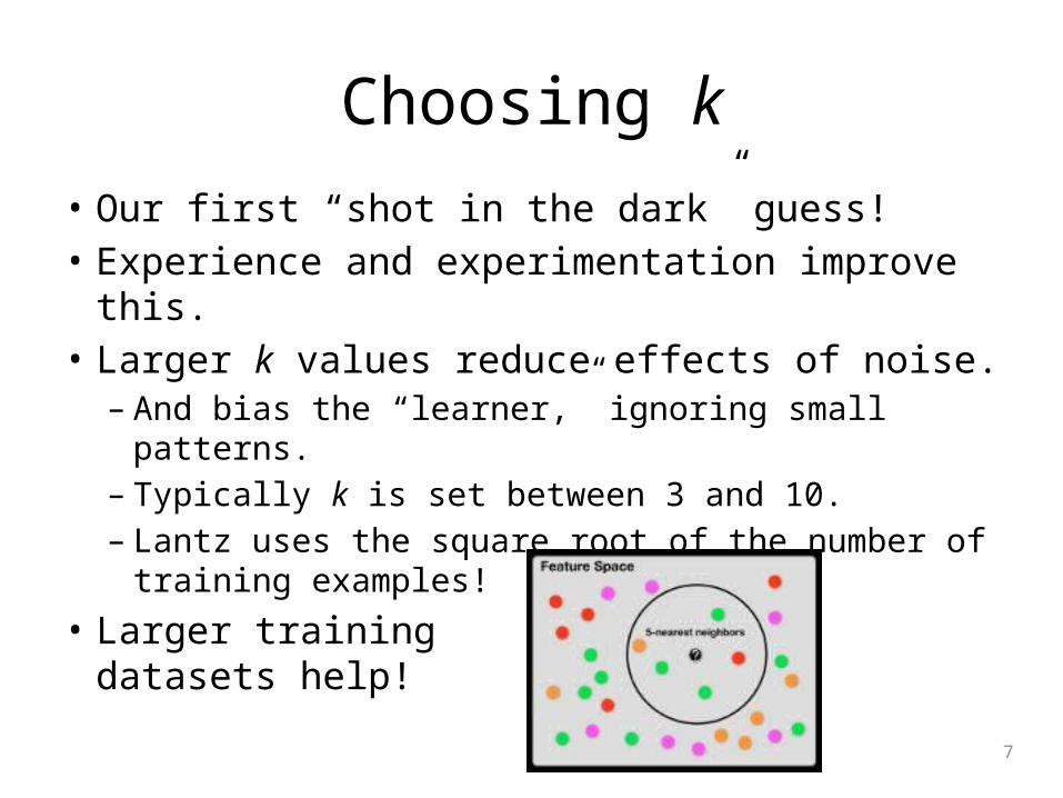
Choosing k

• Our first “shot in the dark” guess!• Experience and experimentation improve this.• Larger k values reduce effects of noise.– And bias the “learner,” ignoring small patterns.– Typically k is set between 3 and 10.– Lantz uses the square root of the number of

training examples!• Larger training

datasets help!

8

Need to “scale” the data

• Usually assume features should contribute equally.– Therefore should be on equivalent scales.

– Using mean and standard deviation may be even better!

9

How to scale “nominal” data

• Bananas are green -> yellow -> brown -> black.– Could be 1 -> 2 -> 3 -> 4.

• But not every nominal variable is easy to convert to some kind of scale.– E.g., What color a car is, versus owner satisfaction.

• “Dummy coding” requires some thought.

10

Why kNN is “lazy”

• It doesn’t provide an abstraction as the “learning”.– “generalization” is on a case-by-case basis.– It’s not exactly “learning” anything.– Just uses the training data, verbatim.

• So, fast training, but slow predictions.– Both take O(n) time.

• It’s like “rote learning.”• It’s “non-parametric”

11

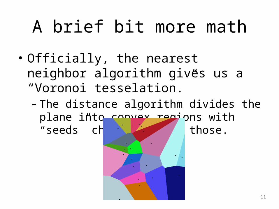
A brief bit more math

• Officially, the nearest neighbor algorithm gives us a “Voronoi tesselation.”– The distance algorithm divides the plane into

convex regions with “seeds” characterizing those.

12

High dimensions are a problem

• If you have lots of features• The spaces tend to be extremely sparse– Every point is far away from every other point– Thus, the pairwise distances are uninformative.

• But, the effective dimensionality may be less– Some of the features may be irrelevant.

13

Lantz’s example – Breast cancer screening

1. Collect the data2. Explore and prepare the data– Transformation – normalize numeric data– Data preparation – creating training and test

datasets

3. Training a model on the data4. Evaluating model performance5. Improving model performance– Transformation – z-score standardization

14

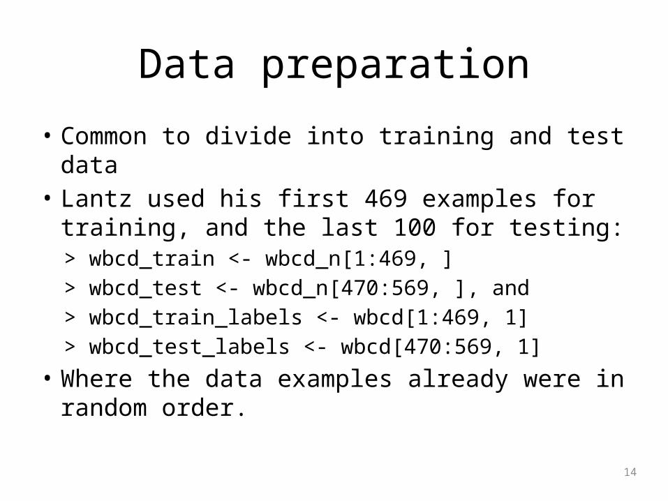
Data preparation

• Common to divide into training and test data• Lantz used his first 469 examples for training,

and the last 100 for testing:> wbcd_train <- wbcd_n[1:469, ]> wbcd_test <- wbcd_n[470:569, ], and> wbcd_train_labels <- wbcd[1:469, 1]> wbcd_test_labels <- wbcd[470:569, 1]

• Where the data examples already were in random order.

15

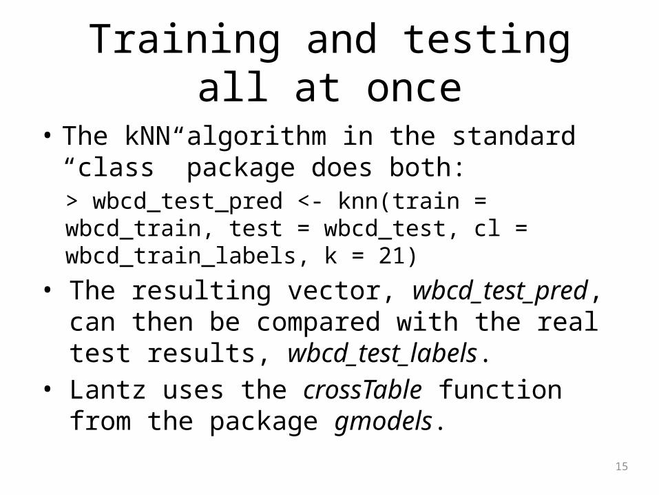
Training and testing all at once

• The kNN algorithm in the standard “class” package does both:> wbcd_test_pred <- knn(train = wbcd_train, test = wbcd_test, cl = wbcd_train_labels, k = 21)

• The resulting vector, wbcd_test_pred, can then be compared with the real test results, wbcd_test_labels.

• Lantz uses the crossTable function from the package gmodels.

16

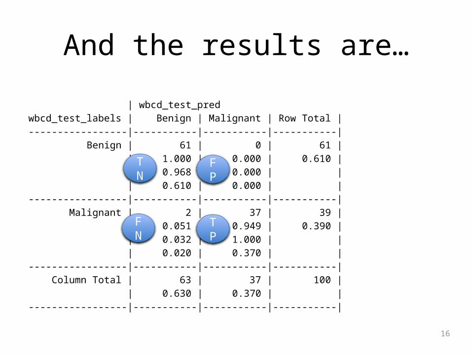
And the results are…

| wbcd_test_pred wbcd_test_labels | Benign | Malignant | Row Total | -----------------|-----------|-----------|-----------| Benign | 61 | 0 | 61 | | 1.000 | 0.000 | 0.610 | | 0.968 | 0.000 | | | 0.610 | 0.000 | | -----------------|-----------|-----------|-----------| Malignant | 2 | 37 | 39 | | 0.051 | 0.949 | 0.390 | | 0.032 | 1.000 | | | 0.020 | 0.370 | | -----------------|-----------|-----------|-----------| Column Total | 63 | 37 | 100 | | 0.630 | 0.370 | | -----------------|-----------|-----------|-----------|

TN

FN

FP

TP