1

Ka-fu WongUniversity of Hong Kong

EViews Commands that are useful for Assignment #2

2

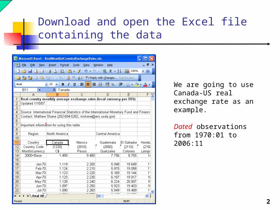
Download and open the Excel file containing the data

We are going to use Canada-US real exchange rate as an example.

Dated observations from 1970:01 to 2006:11

3

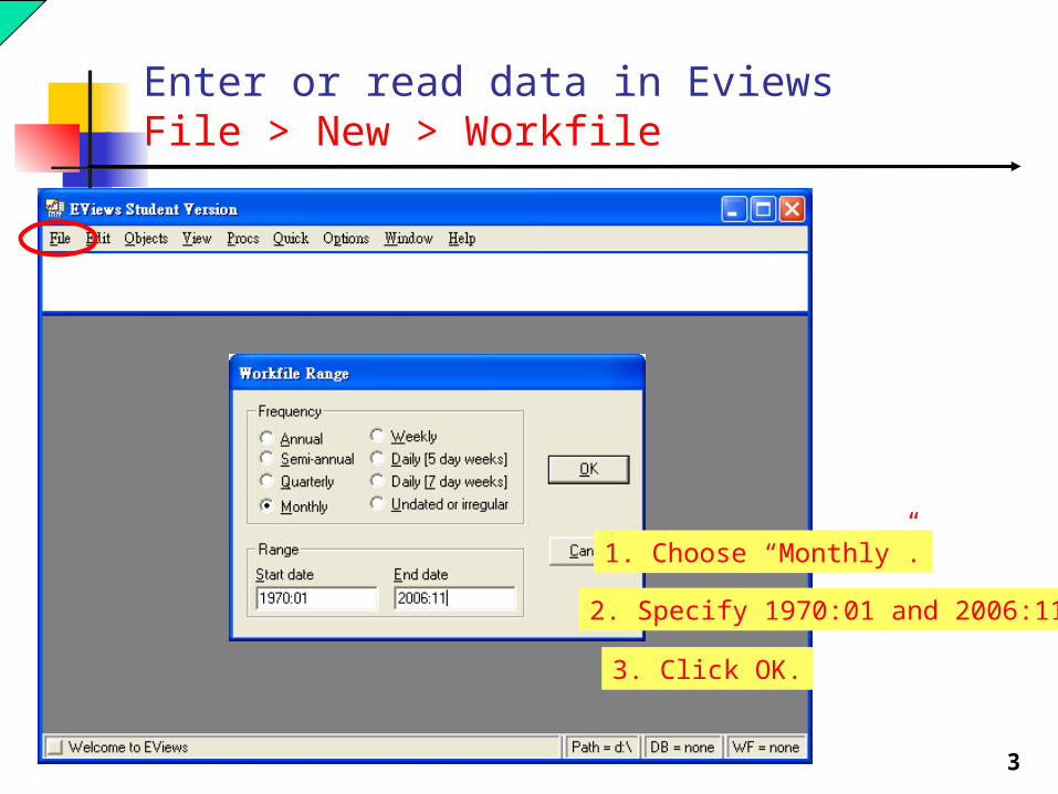
Enter or read data in EviewsFile > New > Workfile

3. Click OK.

1. Choose “Monthly”.

2. Specify 1970:01 and 2006:11

4

Enter or read data in Eviews Choose Quick>Empty Group(Edit Series)

5

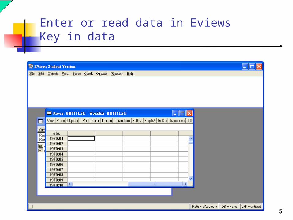
Enter or read data in Eviews Key in data

6

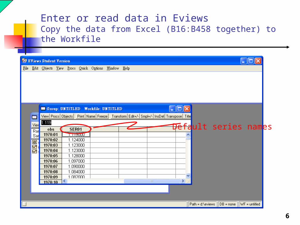
Enter or read data in Eviews Copy the data from Excel (B16:B458 together) to the Workfile

Default series names

7

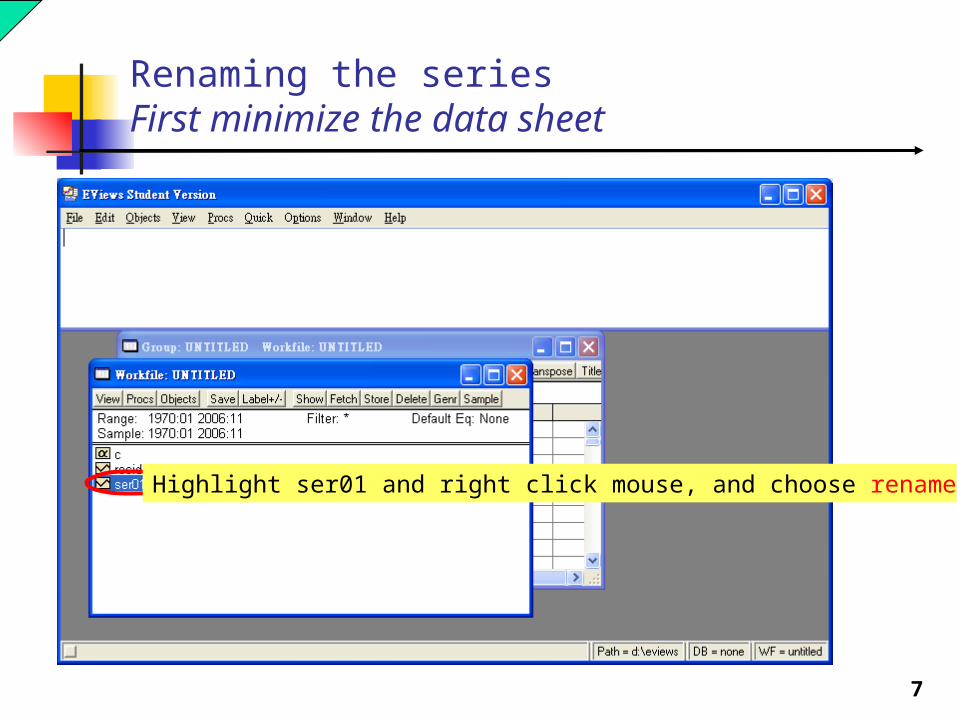
Renaming the seriesFirst minimize the data sheet

Highlight ser01 and right click mouse, and choose rename

8

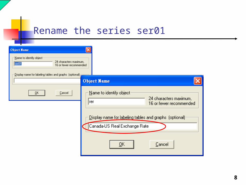
Rename the series ser01

9

Check if the variable names has been changed

10

Save data and results frequently to avoide loss of dataFile>SaveAs

Enter rer1.wf1

11

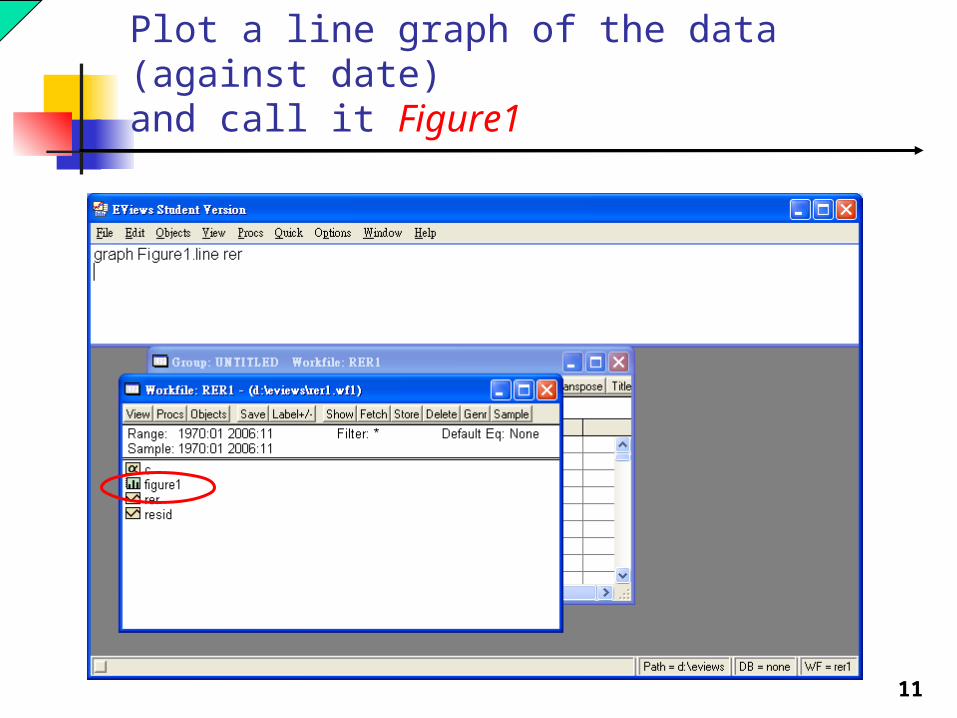
Plot a line graph of the data (against date)and call it Figure1

12

Double click figure1 to see the plot

13

Generate the variable TIME and its relativesTIME=1 for 1970m01 and 2 for 1970m02, etc.

14

Generate the variable TIME and its relativesTIME2, TIME3, TIME4, TIME5

15

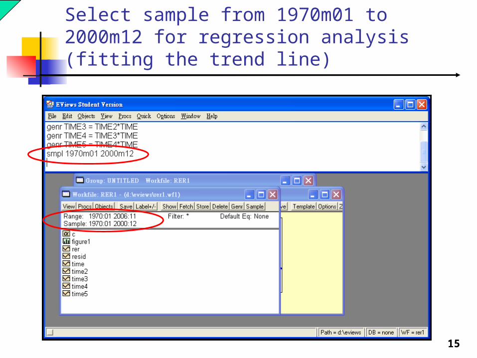
Select sample from 1970m01 to 2000m12 for regression analysis (fitting the trend line)

16

Fit a linear trend using Least Squares and put the result to Table1

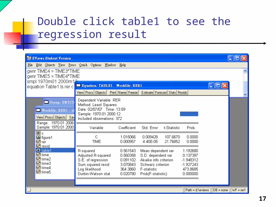
17

Double click table1 to see the regression result

18

Fit Polynomial trend line of various degree (up to 5) using Least Squares and put the result to corresponding tables.

19

Fitting an exponential trend and put result to Table6

20

Plot (in-sample) residuals, fitted values and actual values, and put them in corresponding figures (FigureA?)

21

Generate a new variable containing the historical values of rer from 1970:01 to 2000:12

22

Specify the sample to create out-of-sample forecast

23

Produce a forecast for the sample period 2001m01 to 2006m11 using the Table1 regression results

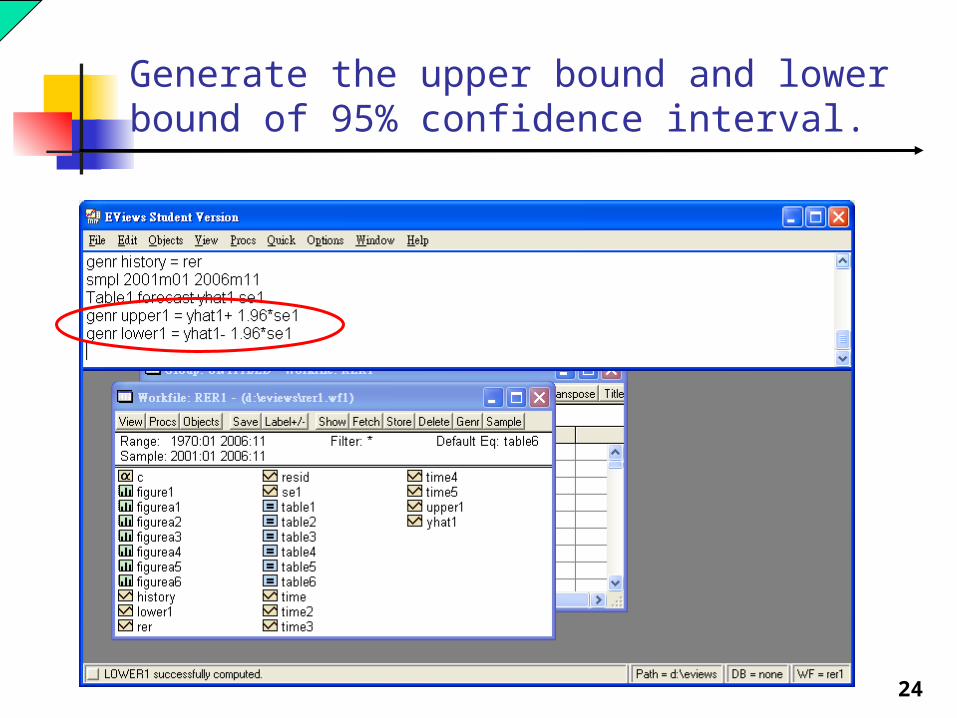
24

Generate the upper bound and lower bound of 95% confidence interval.

25

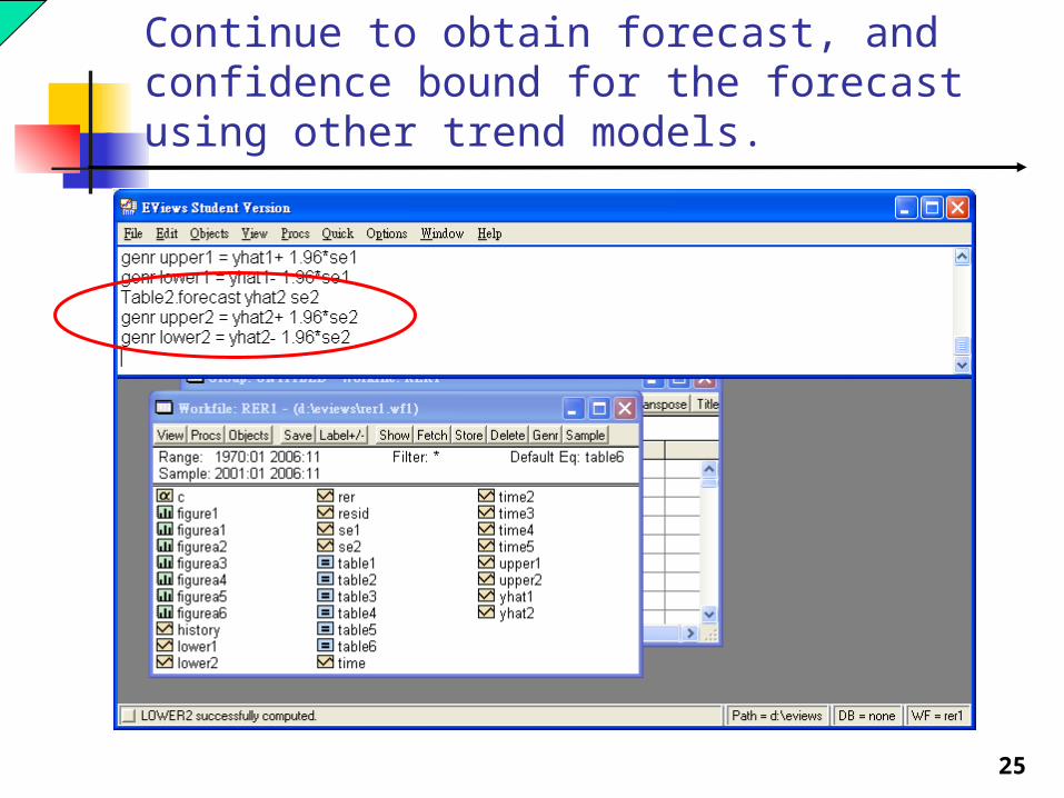
Continue to obtain forecast, and confidence bound for the forecast using other trend models.

26

Change the sample to 1970m01 2006m11, for plotting actual value and forecast together

27

Plot the historical values, forecast, confidence interval and the actual value during the forecasting period.

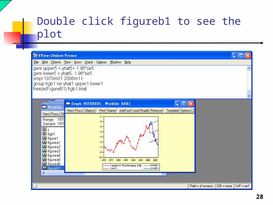
28

Double click figureb1 to see the plot

29

Fix the sample and compute the sqaured forecast errors based on different models.

30

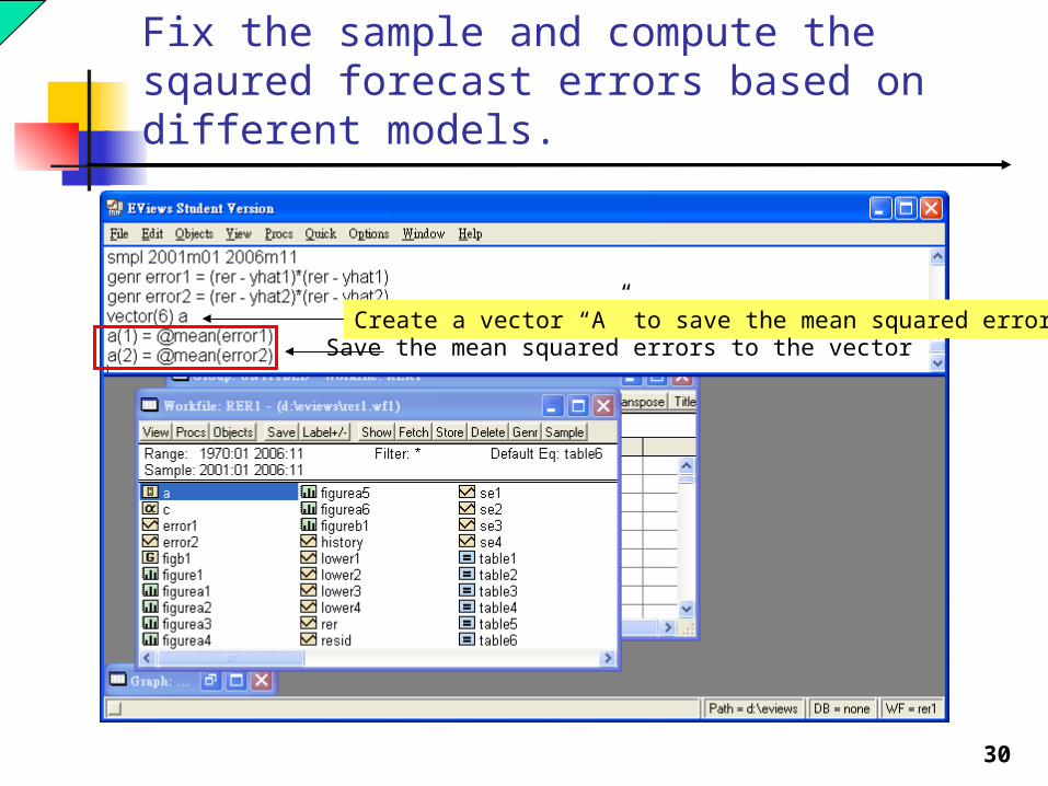
Fix the sample and compute the sqaured forecast errors based on different models.

Create a vector “A” to save the mean squared errors.Save the mean squared errors to the vector

31

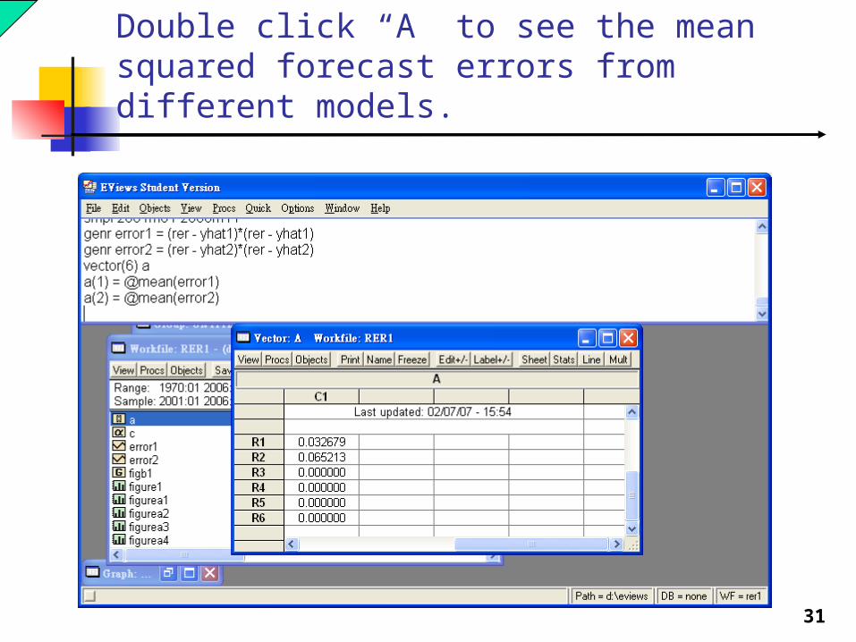
Double click “A” to see the mean squared forecast errors from different models.

32

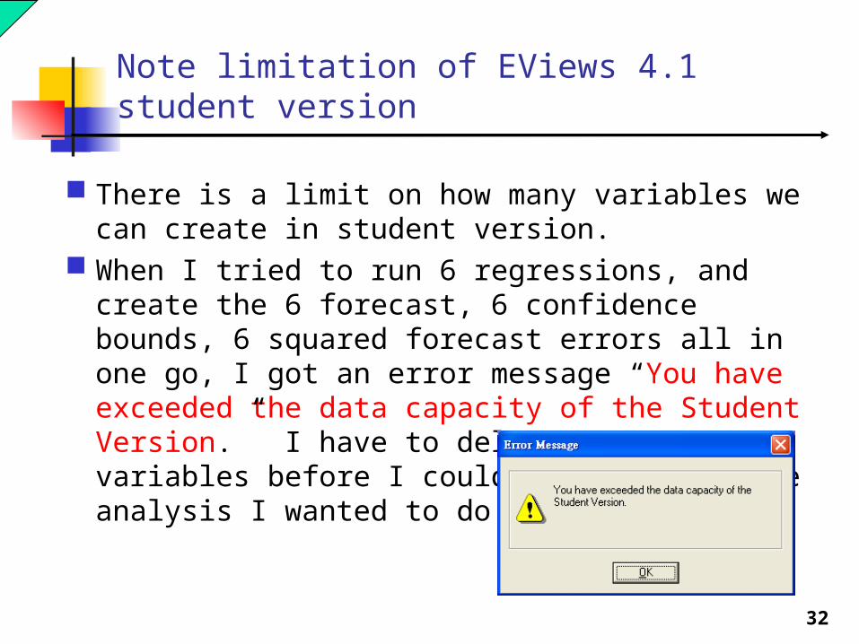
Note limitation of EViews 4.1 student version

There is a limit on how many variables we can create in student version.

When I tried to run 6 regressions, and create the 6 forecast, 6 confidence bounds, 6 squared forecast errors all in one go, I got an error message “You have exceeded the data capacity of the Student Version.” I have to delete some variables before I could complete all the analysis I wanted to do.

33

End