FRTN10 Multivariable Control

Laboratory Session 3

Kalman Filtering and LQ Control of the MinSeg Robot1

Department of Automatic Control

Lund University

1. Introduction

In this laboratory session we will develop Kalman filters and a linear-quadratic (LQ)controller for the MinSeg™ balancing robot, see Figure 1.

Figure 1 The MinSeg™ balancing robot.

The aim of the lab is to develop a working controller for balancing the robot and letit follow a square-wave wheel position reference signal. We will first design two Kalmanfilters to extract state information from the raw gyro, accelerometer, and wheel encodersignals. Then we will design an LQ controller for state feedback from the estimated stateswith optional integral action and reference tracking.

Pre-lab assignments

Read this document and complete all assignments marked as (Preparatory). Helpful lec-tures to review are lectures 9–11 on LQ control, Kalman filtering, and LQG control. Partsof lecture 3 concerning stochastic processes and their spectrum are also useful.

1Written by Anton Cervin, latest update October 10, 2018.

1

Figure 2 Definition of x, y, and z axes, tilt angle α and wheel angle θ (adapted from [1]).

2. The Process

The drivetrain of the MinSeg is a Lego NXT DC motor equipped with wheels. An ArduinoMega 2560 microcontroller drives the motor and reads sensor data. During the lab theMinSeg will be connected top a PC via a USB connector which allows the Arduino tobe programmed and enables the reading of plot data and writing of parameters duringruntime.

The MinSeg is equipped with to sensor units. The first is a rotational encoder, built intothe Lego NXT motor, which gives the wheels rotational position around the wheel axle,we call this angle θ. In the conditions of the lab, no wheel slippage will occur and thisangle the directly corresponds to backward and forward position of the robot.

The second sensor unit is the inertial measurement unit (IMU). It is part of the addon board on top of the Arduino Mega. An IMU consists of two sensors: a gyro and anaccelerometer. A gyro gives the angular velocities around it’s coordinate axes while theaccelerometer gives the acceleration along the axes. Figure 2 shows the x, y and z axes ofthe IMU’s coordinate system. Figure 2 also shows the robots tilt angle, α.

In order to properly control the process an accurate estimate of it’s state needs to befound. Without going into details of the dynamics of the system, we say that the stateconsists of four state variables: The angle of rotation of the wheels, θ, and the tilt angle,α, as well as their time derivatives. Since we only measure two of these states directly, θand α, and both of those measurements are noisy, the state estimate needs to be formedby filtering of the data provided from the IMU and wheel encoder.

3. The Lab Interface

We will use Simulink with Simulink Coder (formerly Real-Time Workshop) for modelingand implementation of the filters and controllers. The main diagram is shown in Figure 3.

The model is configured by five variables in the Matlab workspace, these variables are

2

u

Motor

theta_enc

Wheel encoder

x1,x2

alphadot_gyro

alpha_accel

IMU

IMU_Kalman_D

IMU Kalman filter u

K*u

Feedback gain

x3,x4,ref

Wheel_Kalman_D

Wheel Kalman filter

0

Output gain

K Ts

z-1Integrator

-K-Integral gain

theta

reference

Figure 3 Simulink model lab3.slx for filter and controller implementation.

IMU Kalman D, Wheel Kalman D, Feedback Gain, Integral Gain, and Ts. When the simulinkmodel is run, it will read these variables, compile the resulting controller and upload itto the MinSeg. To design our controller we simply assigning different kalman filters andfeedback gains to the workspace variables. When the model is first opened, default (zero)values for the controller variables automatically defined.

The last variable, Ts, is the sample time for the controller. In the first part of the lab thiswill be set to 40 ms but later you will be asked to decrease it to 15 ms. This is because thescopes of Simulink model are not able to update properly at the higher sample frequencyso in order to properly look at our measurements the longer sample time is needed. Whenwe later tries to actually control the process, better performance is achieved with the fastersample time.

Assignment 1. Download lab3 files.zip from the course homepage and extract thecontents to some suitable working directory. In a terminal window, type

VERSION=R2016a matlab

to start Matlab R2016a. Once Matlab has started, go into the lab3 files directory and then type

setup lab3

to setup the paths to the Matlab/Simulink support packages and the Simulink libraries for theArduino and MinSeg hardware.

Open up and explore the Simulink model lab3.slx. Make sure that you understand how the IMU,Wheel encoder and Motor blocks relate to the real MinSeg robot. Also check the current value ofTs. it should be 40 ms. ✷

4. Tilt Angle Measurements

First we will focus on the measurements that will form our estimation of the tilt angle, α, and it’sderivative, α. These measurements will be taken from the IMU. The gyro gives us a noisy signalproportional to α, while the accelerometer data together with some trigonometry can give a roughestimate of α.

3

4.1 Calibration

The IMU needs to be calibrated. Both the gyro and the accelerometer has an offset that needs tobe corrected by adding a bias to the raw signal. This offset can also drift slightly so the IMU mightneed recalibration during the lab.

Assignment 2. Connect the MinSeg to the computer using the USB cable. Check that the COMport is properly defined in the Simulink model under Simulation / Model Configuration Parameters/ Hardware Implementation / Host-board connection. (Switching from Manually to Automatically andback to Manually again normally sets it right.)

Click “Run” in the Simulink model and wait about 60 seconds for the diagram to be compiled anduploaded to the Arduino. (If you get an error message, ask the lab supervisor for help.) When themodel is running, open up the IMU subsystem and study the raw signals from the x gyro and fromthe z and y accelerometers. Rotate the robot in different directions by hand and verify that thesignals seem to behave as expected. ✷

Assignment 3. Lay the robot flat on its back (battery case towards the table) and calibratethe x gyro and y accelerometer readings to zero (approximately, on average) by entering suitablevalues for the offsets xvel bias and yaccel bias. Then stand the robot up and hold the battery casetowards a vertical surface, e.g. a wall, and calibrate the z accelerometer reading to zero by similarlyadjusting zaccel bias. ✷

The raw values of the gyro and the accelerometer can drift slightly so this calibration procedureabove might be needed to be repeated.

4.2 Angle Measurement

The gyro gives us a direct, but noisy, measurement of the angular velocity, i.e. α, but we have nodirect measurement of α. A rough estimate can be formed by looking at the components of theacceleration data given by the accelerometer.

When the device is sitting still, the three acceleration components ax, ay, and az will add up as

√

a2x + a2y + a2z = 9.81 m/s2

As long as the robot is stationary and not tilting sideways (ax = 0), we can use the geometricrelationship indicated in Figure 2 and calculate the tilt angle according to

α = atan2(az ,−ay)

The accelerometer signals are noisy and they also pick up any external forces acting on the IMUchip (remember F = m ·a), making the calculation above meaningful only for low-frequency signalcomponents (below, say, 1 rad/s).

Assignment 4. Look at the alpha accel scope in the IMU block of the Simulink model. Doesthe measurement correctly describe the tilt angle when the MinSeg is stationary? Move the MinSegforward and backward without tilting it, is the measurement of the angle correct? ✷

4.3 Measurement Noise Identification

The IMU block in the Simulink model returns the calibrated and rescaled values of α and α andthese are now considered as two of our noisy measurements. In order to design good filters wewould like to know more about the noise characteristics.

Assignment 5. Keep the robot completely still for 1000 · Ts seconds and then hit “Stop”.The 1000 most recent measurements are automatically stored in the workspace in the variables ofalphadot gyro and alpha accel. For the first measurement (alphadot gyro), plot the signals, removeany linear trends, calculate their variance and save it in variable, and plot their spectra, using:

4

wα α α

n1 n2∑∑

y1 y2

1

s

1

s

Figure 4 Model of the IMU for design of the first Kalman filter.

plot(alphadot gyro) % plot

y1 = detrend(alphadot gyro,'linear'); % remove linear trend

plot(y1) % plot again

y1var = var(y1); % calculate stationary variance

pwelch(y1) % plot periodogram (estimate of spectrum)

Is the measurement noise white? What is the intensity? Answer the same questions for the mea-surement given by alpha accel. Make sure to save y1var and y2var for later use. ✷

5. Tilt Angle Estimation

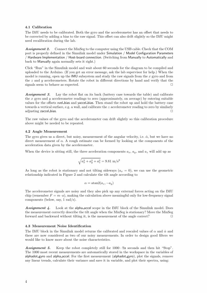
We will use a Kalman filter to reduce the effect of the noise on our measurements y1 and y2 of αand α. Kalman filters need a model of the dynamics and the simplest possible choice is to simplyconsider the robot dynamics as completely unknown and describe them some process noise in theform of external angular acceleration wα. The system can then be modeled as a double integratorfrom wα to the tilt angle α, see Figure 4.

wα contain all dynamics from the motor and the inverted pendulum and is in reality very non-whitenoise. However, since the aim was simplicity we will assume it is white noise with intensity R1.The downside of this modeling choice is of course that the resulting filter won’t be as good as itcould be but it will be adequate for this application.

Assignment 6 (Preparatory). Convert the model in Figure 4 to state-space form usingthe state vector ( x1

x2) = ( αα ). What dimensions and structure do the process and measurement

noise intensity matrices R1, R2, and R12 have in this case? Assume that the noise processes areuncorrelated.

Setting R2 = I, write down the algebraic Riccati equation and the resulting set of quadraticequations involving the elements of the error covariance matrix P = ( p1 p2

p2 p3). Would it be easy to

solve these equations by hand?

Using lqe in Matlab, calculate the Kalman filter gain K and the resulting observer poles for somedifferent values of R1 (very large and very small). How is the relative size of R1 compared to R2

influencing the speed of the observer? ✷

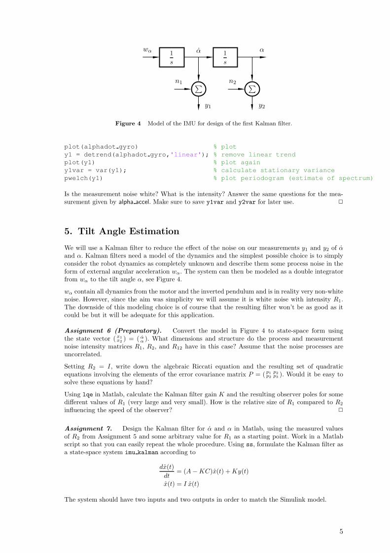
Assignment 7. Design the Kalman filter for α and α in Matlab, using the measured valuesof R2 from Assignment 5 and some arbitrary value for R1 as a starting point. Work in a Matlabscript so that you can easily repeat the whole procedure. Using ss, formulate the Kalman filter asa state-space system imu kalman according to

dx(t)

dt= (A−KC)x(t) +Ky(t)

x(t) = I x(t)

The system should have two inputs and two outputs in order to match the Simulink model.

5

wθ θ θ

n3

∑

y31

s

1

s

Figure 5 Model of the wheels for design of the second Kalman filter.

Plot the Bode magnitude diagram of the filter using bodemag and interpret what you see. How arethe measurements y1 and y2 combined to produce the estimates x1 and x2 respectively?

Finally, convert the filter into a discrete-time system IMU Kalman D using c2d and first-order holdsampling1 as follows:

IMU Kalman D = c2d(imu kalman, Ts, 'foh');

“Run” the Simulink model and try the Kalman filter on the real process. Tilt the robot by handand observe how fast the estimates x1 and x2 are following the movements. Hit “Stop”, repeat thewhole procedure with different design matrices and observe the difference in tracking speed. Forbalancing, the filter bandwidth from y1 to x1 should be at least 50 rad/s and from y2 to x2 about1 rad/s. ✷

6. Wheel Position Estimation

With a filter for two of our state variables, we turn to designing a second Kalman filter for estimatingthe wheel angular speed θ and position θ. For this we will rotational encoder of the motor whichwill be our last measurement y3.

Similar to to before model most of the dynamics as unknown process noise on a double integrator.As before the noise contains the response of the motor on changes in the applied voltage and theinertia of the robot. A model of the subsystem is shown in Figure 5.

Different from before we now only have one measurement, the output from the encoder. This signalis not very noisy but is quantized with a resolution of 0.5 degrees which results in uncertainties.The measurement noise of the model, n3, represents this quantization error of the wheel encoder.

Assignment 8 (Preparatory). Convert the model in Figure 5 to state-space form using thestate vector ( x3

x4) =

(

θθ

)

. Assuming the relative noise intensities

R1 =

ω4 0

0 0

, R2 = 1,

show that the algebraic Riccati equation for the Kalman filter has the solution

P =

√2ω3 ω2

ω2√2ω

and that the resulting observer poles are given by the characteristic equation

s2 +√2ωs+ ω2 = 0.

(We have hence shown that, for this problem, placing the two observer poles in the standard patternwith ±45◦ angle from the negative real axis is optimal.) ✷

1You can learn more about discretization and implementation methods in FRTN01 Real-Time Systems.

6

Assignment 9. Design the Kalman filter for θ and θ in Matlab. Aim for a filter bandwidthof at least 50 rad/s. Formulate the Kalman filter as a state-space system wheel kalman using ss

(see Assignment 6). The system should in this case have one input and two outputs to match theSimulink model. Then convert it into discrete time and save it to Wheel Kalman D using

Wheel Kalman D = c2d(wheel kalman, Ts, 'foh');

Finally, hit “Run” and try the Kalman filter on the real process. Turn the robot wheels by handand verify that the estimates x3 and x4 seem to behave as expected. ✷

7. Design of LQ State Feedback

With filters for all of our state variables ee now turn to modeling and controlling the dynamics ofthe robot to make it balance in the upright position (α = 0).

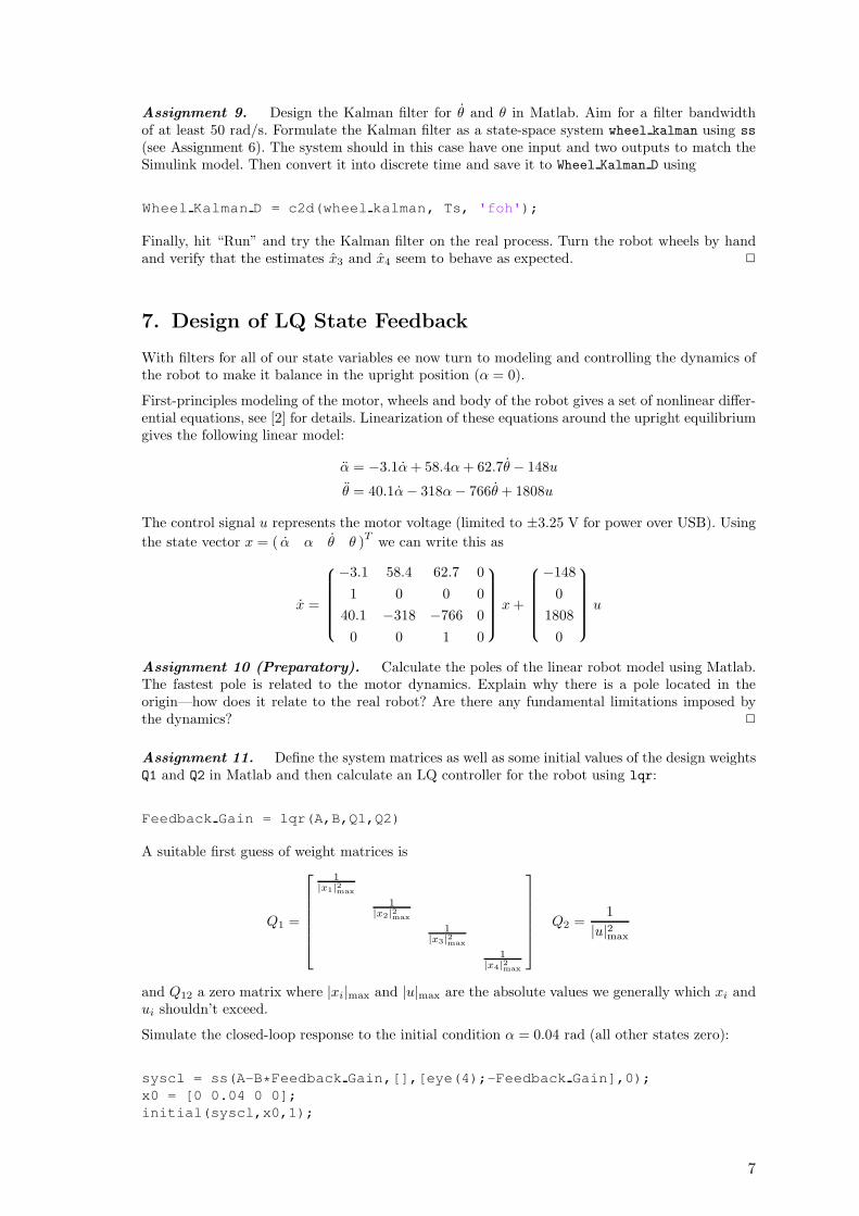
First-principles modeling of the motor, wheels and body of the robot gives a set of nonlinear differ-ential equations, see [2] for details. Linearization of these equations around the upright equilibriumgives the following linear model:

α = −3.1α+ 58.4α+ 62.7θ− 148u

θ = 40.1α− 318α− 766θ+ 1808u

The control signal u represents the motor voltage (limited to ±3.25 V for power over USB). Using

the state vector x = ( α α θ θ )Twe can write this as

x =

−3.1 58.4 62.7 0

1 0 0 0

40.1 −318 −766 0

0 0 1 0

x+

−148

0

1808

0

u

Assignment 10 (Preparatory). Calculate the poles of the linear robot model using Matlab.The fastest pole is related to the motor dynamics. Explain why there is a pole located in theorigin—how does it relate to the real robot? Are there any fundamental limitations imposed bythe dynamics? ✷

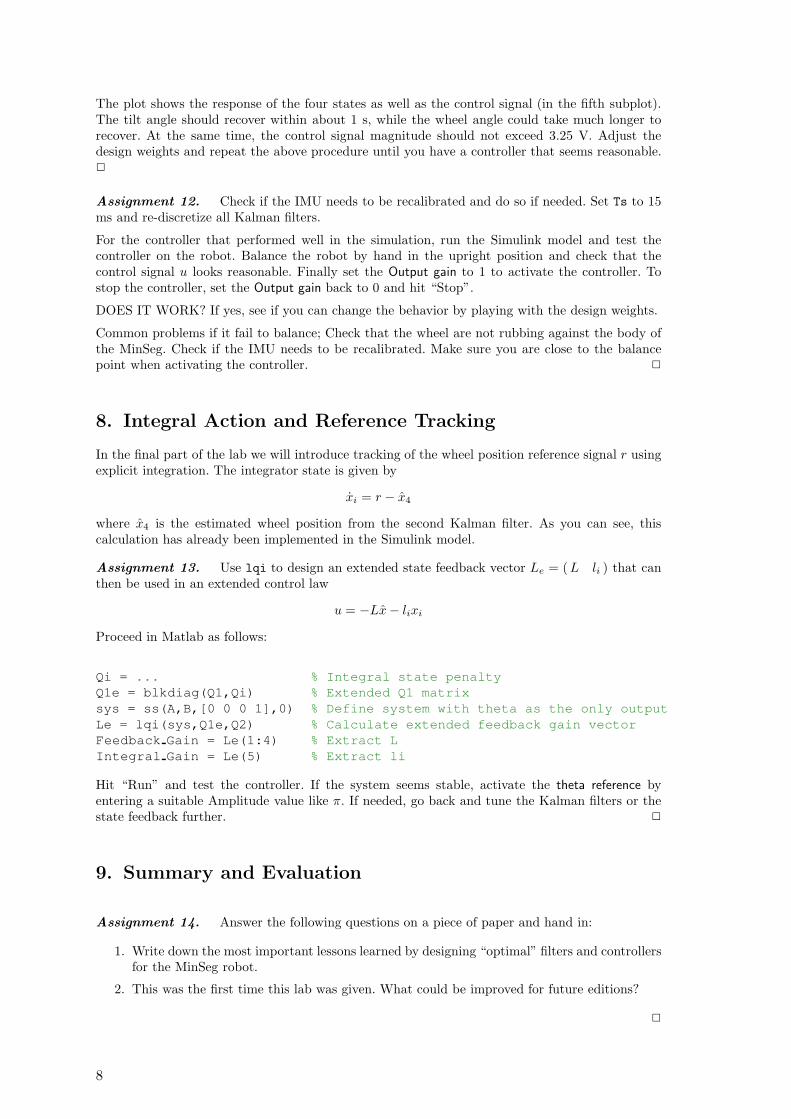
Assignment 11. Define the system matrices as well as some initial values of the design weightsQ1 and Q2 in Matlab and then calculate an LQ controller for the robot using lqr:

Feedback Gain = lqr(A,B,Q1,Q2)

A suitable first guess of weight matrices is

Q1 =

1

|x1|2max

1

|x2|2max

1

|x3|2max

1

|x4|2max

Q2 =1

|u|2max

and Q12 a zero matrix where |xi|max and |u|max are the absolute values we generally which xi andui shouldn’t exceed.

Simulate the closed-loop response to the initial condition α = 0.04 rad (all other states zero):

syscl = ss(A-B*Feedback Gain,[],[eye(4);-Feedback Gain],0);

x0 = [0 0.04 0 0];

initial(syscl,x0,1);

7

The plot shows the response of the four states as well as the control signal (in the fifth subplot).The tilt angle should recover within about 1 s, while the wheel angle could take much longer torecover. At the same time, the control signal magnitude should not exceed 3.25 V. Adjust thedesign weights and repeat the above procedure until you have a controller that seems reasonable.✷

Assignment 12. Check if the IMU needs to be recalibrated and do so if needed. Set Ts to 15ms and re-discretize all Kalman filters.

For the controller that performed well in the simulation, run the Simulink model and test thecontroller on the robot. Balance the robot by hand in the upright position and check that thecontrol signal u looks reasonable. Finally set the Output gain to 1 to activate the controller. Tostop the controller, set the Output gain back to 0 and hit “Stop”.

DOES IT WORK? If yes, see if you can change the behavior by playing with the design weights.

Common problems if it fail to balance; Check that the wheel are not rubbing against the body ofthe MinSeg. Check if the IMU needs to be recalibrated. Make sure you are close to the balancepoint when activating the controller. ✷

8. Integral Action and Reference Tracking

In the final part of the lab we will introduce tracking of the wheel position reference signal r usingexplicit integration. The integrator state is given by

xi = r − x4

where x4 is the estimated wheel position from the second Kalman filter. As you can see, thiscalculation has already been implemented in the Simulink model.

Assignment 13. Use lqi to design an extended state feedback vector Le = (L li ) that canthen be used in an extended control law

u = −Lx− lixi

Proceed in Matlab as follows:

Qi = ... % Integral state penalty

Q1e = blkdiag(Q1,Qi) % Extended Q1 matrix

sys = ss(A,B,[0 0 0 1],0) % Define system with theta as the only output

Le = lqi(sys,Q1e,Q2) % Calculate extended feedback gain vector

Feedback Gain = Le(1:4) % Extract L

Integral Gain = Le(5) % Extract li

Hit “Run” and test the controller. If the system seems stable, activate the theta reference byentering a suitable Amplitude value like π. If needed, go back and tune the Kalman filters or thestate feedback further. ✷

9. Summary and Evaluation

Assignment 14. Answer the following questions on a piece of paper and hand in:

1. Write down the most important lessons learned by designing “optimal” filters and controllersfor the MinSeg robot.

2. This was the first time this lab was given. What could be improved for future editions?

✷

8

References

[1] Angle estimation using gyros and accelerometers (lab PM), January, 2018. Division of Auto-matic Control, ISY, Linkoping University, Sweden.

[2] Brian Howard and Linda Bushnell. Enhancing linear system theory curriculum with an invertedpendulum robot. In Proc. American Control Conference, 2015.

9