1 introduction ijser · takeaki nadabe, nobuo takeda abstract — in this study, a model of fiber...

International Journal of Scientific & Engineering Research, Volume 5, Issue 5, May-2014 553 ISSN 2229-5518

IJSER © 2014 http://www.ijser.org

Modeling of Fiber Microbuckling in Composite Materials

Takeaki Nadabe, Nobuo Takeda

Abstract— In this study, a model of fiber microbuckling in composite materials is proposed for the purpose of material strength analysis. Firstly the fiber microbuckling is numerically simulated using finite element method in order to understand how this deformation phenomenon appears in the material. Then the equations expressing deformation of composite materials are compiled, and the correspondence between the equations and the actual deformation phenomenon in composite materials are considered. It is indicated that onset of arbitrariness in solution of equations expressing the deformation of composite materials is closely related with the initiation of the fiber microbuckling in composite materials and thus the material strength of composite materials.

Index Terms— Fiber microbuckling, material strength, nonlinear deformation, composite materials

—————————— ——————————

1 INTRODUCTION OMPOSITE materials commonly have complex internal structures including fibers, matrix, interfaces and inter-laminar regions, and when precise evaluation of fracture

strength of the material is conducted, the internal fracture pro-cess in the materials is necessary to be taken into account in the numerical analysis [1]. In recent years, composite materials are being increasingly used in several industrial fields, and the precise evaluation of mechanical response of the material un-der various loading condition and environmental condition increases the necessity in design and improvement of indus-trial products [2]. Compressive failure is one of the typical failure modes in fiber reinforced composite materials [3], and fracture strength in compressive failure often becomes one of the limiting factors at the design phase of structural elements [4]. Not only uniaxial compressive strength but also compres-sive strength at around open holes and post-impact compres-sive strength in the materials are related to the fundamental compressive strength of the materials, and improvement of compressive strength would be related with the increase of the light weight potential of the materials. In this study, a model of fiber microbuckling in composite materials is proposed. Firstly the fiber microbuckling is numerically simulated using finite element method to understand how this deformation phenomenon appears in the material, and then the model of this phenomenon is considered.

2 NUMERICAL SIMULATION OF FIBER MICROBUCKLING 2.1 Numerical Model In order to investigate the physical mechanism of fiber mi-

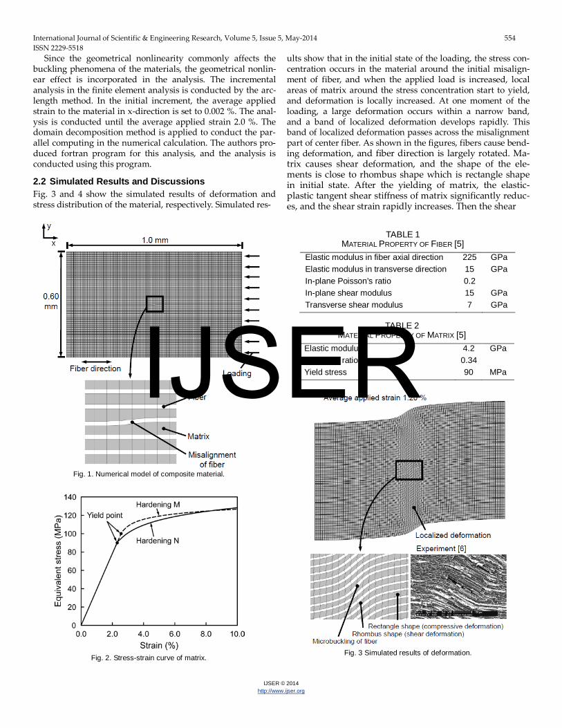
crobuckling in composite materials, the numerical simulation of fiber microbuckling is conducted. Finite element method is used to simulate the fiber microbuckling. Fig. 1 shows the numerical model of this analysis. The white and gray elements in Fig. 1 represent fibers and matrix, respectively. The thick-ness of the ply in y-direction is 0.60 mm. The length in x-direction is 1.0 mm, and the thickness in z-direction is 100 mm. The diameter of each fiber is set to 3.5 μm, and the interval of fibers is 20.0 μm. The fiber volume fraction of the materials is set to 17.5 %. Each fiber and matrix is modeled by two-dimensional plate elements. The one fiber placed at the center has the initial misalignment as shown in the figure. The initial misalignment of the fiber is introduced using the sine func-tion. The x coordinate of each node is placed regularly at the interval of 5.0 μm, and the y coordinate of each node is calcu-lated using the sine function. The other fibers are modeled as the straight lines and the fiber axial direction is parallel to the x-direction.

Due to the atomic structure in the inside of the fibers, the fibers commonly have the different material property in be-tween fiber axial and transverse directions. Here, the fibers are modeled by the transversely isotropic elastic material. Table 1 shows the material property of the fibers. Carbon fiber AS4 (Hexcel Corp.) is assumed [5]. Matrix is modeled by isotropic elastic-plastic material. Commonly the compressive failure of composite materials is affected by the nonlinear stress-strain relation of matrix, thus in this analysis the nonlinear stress-strain curve of matrix shown in Fig. 2 (hardening curve N) is applied, and the nonlinear finite element analysis is conduct-ed. Table 2 shows the material property of matrix. Epoxy resin 3501-6 (Hercules Chemical Company, Inc.) is assumed [5]. The quasi-static and room temperature environment are assumed in the analysis.

C

———————————————— • Takeaki Nadabe E-mail: [email protected] • Nobuo Takeda E-mail: [email protected]

IJSER

http://www.ijser.org/



Since the geometrical nonlinearity commonly affects the buckling phenomena of the materials, the geometrical nonlin-ear effect is incorporated in the analysis. The incremental analysis in the finite element analysis is conducted by the arc-length method. In the initial increment, the average applied strain to the material in x-direction is set to 0.002 %. The anal-ysis is conducted until the average applied strain 2.0 %. The domain decomposition method is applied to conduct the par-allel computing in the numerical calculation. The authors pro-duced fortran program for this analysis, and the analysis is conducted using this program.

2.2 Simulated Results and Discussions Fig. 3 and 4 show the simulated results of deformation and stress distribution of the material, respectively. Simulated res-

ults show that in the initial state of the loading, the stress con-centration occurs in the material around the initial misalign-ment of fiber, and when the applied load is increased, local areas of matrix around the stress concentration start to yield, and deformation is locally increased. At one moment of the loading, a large deformation occurs within a narrow band, and a band of localized deformation develops rapidly. This band of localized deformation passes across the misalignment part of center fiber. As shown in the figures, fibers cause bend-ing deformation, and fiber direction is largely rotated. Ma-trix causes shear deformation, and the shape of the ele-ments is close to rhombus shape which is rectangle shape in initial state. After the yielding of matrix, the elastic-plastic tangent shear stiffness of matrix significantly reduc-es, and the shear strain rapidly increases. Then the shear

TABLE 1 MATERIAL PROPERTY OF FIBER [5]

Elastic modulus in fiber axial direction 225 GPa Elastic modulus in transverse direction 15 GPa In-plane Poisson’s ratio 0.2 In-plane shear modulus 15 GPa Transverse shear modulus 7 GPa

TABLE 2 MATERIAL PROPERTY OF MATRIX [5]

Elastic modulus 4.2 GPa Poisson’s ratio 0.34 Yield stress 90 MPa

Fig. 3 Simulated results of deformation.

Fig. 2. Stress-strain curve of matrix.

Fig. 1. Numerical model of composite material.

IJSER




deformation of this part of matrix increases, and due to the shear deformation of the part, the band of localized defor-mation is formed. The reduction of tangent shear stiffness of matrix after yielding is the essential factor in the onset of the microbuckling of the fibers.

3 MODELING OF FIBER MICROBUCKLING 3.1 Equations Expressing Deformation of Composite

Materials Here, the equations expressing deformation of composite ma-terials are compiled. The equations consist of motion equation and constitutive equation. The motion equation is represented as the following,

ij

iji fXP

tu

02

2

0 ρρ +∂

∂=

∂∂ (1)

where 0ρ is density, t is time, iu is displacement, jX is co-ordinate at reference configuration, ijP is the first Piola-Kirchhoff stress and if is external force. The nonlinear stress-strain relation of composite materials is represented by the nonlinear deformation theory shown by Tohgo et al. [7].

εCσ dd comp=

( )( ){ } KCSCCCC 11 −+−−= mmffmcomp V (2)

( ) ( ){ } ffmmff VV CCSCCK ++−−= 1 where σd is stress rate, εd is strain rate, compC , fC and mC are constitutive tensors of composites, fibers and matrix, re-spectively, fV is fiber volume fraction and S is Eshelby ten-sor. Next, the effect of geometrical nonlinearity during the material deformation is considered. Here the constitutive ten-sor in spacial description is defined in the relation between the second Piola-Kirchhoff stress and the right Cauchy-Green de-formation tensor.

CGcd

abspaabcd C

SC∂∂

= (3)

where spaabcdC is constitutive tensor in spacial description, abS is

the second Piola-Kirchhoff stress and CGcdC is the right Cauchy-

Green deformation tensor. The constitutive tensor in material description is represented by the constitutive tensor in spacial description as follows,

spaabcdldkcjbia

matijkl CFFFFJC 12 −=

spaabcd

d

l

c

k

b

j

a

i CXx

Xx

Xx

Xx

J ∂∂

∂∂

∂

∂

∂∂

=12 (4)

where matijklC is constitutive tensor in material description, iaF

is deformation gradient, ijFJ det= is Jacobian and ix is coor-dinate at present configuration. Cauchy stress is represented by the second Piola-Kirchhoff stress, deformation gradient and Jacobian as follows,

jlklikij FSFJ 1−=σ (5)

jlklikjlklikij FSFJFSFJ 11 −− +=σ

jlklikjlklik FSFJJFSFJ 11 −− −+ (6) where ijσ is Cauchy stress and ijσ is the material time deriva-tive of Cauchy stress. Here, the time derivative of deformation gradient and Jacobian is

kjikij FLF = , iiLJ = (7) where ikL is velocity gradient. Then

jlklikjlklmkimij FSFJFSFLJ 11 −− +=σ

jlklikmmjmmlklik FSFLJLFSFJ 11 −− −+

llijjkikkjikjlklik LLLFSFJ σσσ −++= − 1 (8) where

onomspaklmnonom

spaklmn

CGmn

spaklmnkl FFCFFCCCS +=⋅=

pnopomspaklmnonpmop

spaklmn FLFCFFLC += (9)

opspaklmnonpmjlikjlklik LCFFFFJFSFJ 11 −− =

opspaklmnpnomjlik LCFFFFJ 1−+

opmatijopop

matijpo LCLC

21

21

+=

( ) klmatijklkllk

matijkl DCLLC =+⋅=

21 (10)

Therefore llijjkikkjikkl

matijklij LLLDC σσσσ −++= (11)

This coinsides with the formulation of Truesdell rate of Cau-chy stress. There, here the formulation of finite deformation is

Fig. 4 Simulated results of stress distribution.

IJSER




based on Truesdell rate of Cauchy stress. Then the rate of the first Piola-Kirchhoff stress is represented as follows,

( )klilllikikk

jij LL

xX

JP σσσ −+∂

∂=

( )illmklmatimkl

m

j LDCxX

J σ+∂

∂=

( )l

kiklm

matimkl

m

j

xuC

xX

J∂∂

+∂

∂=

δσ (12)

where ikδ is Kronecker delta. From (1) and (12), a set of equa-tions expressing deformation of composite materials is ob-tained.

ij

iji fXP

tu

02

2

0 ρρ +∂

∂=

∂∂ (13)

( )l

kiklm

matimkl

m

jij x

uCxX

JP∂∂

+∂

∂=

δσ (14)

3.2 Arbitrariness Appearing in Solution of Equations in Deformation of Composite Materials

Equations (13) and (14) are unified to one differential equation.

∂∂

∂∂

=−∂∂

l

kijkl

ji

i

xuA

Xf

tu

02

2

0 ρρ (15)

where tensor ijklA is

( )iklmmatimkl

m

jijkl C

xX

JA δσ+∂

∂= (16)

Equation (15) plays a role of governing equation in the defor-mation of composite materials. When the reference configura-tion is taken at the moment of the present time, and in the place where the external force doesn’t act, (15) becomes as follows,

∂∂

∂∂

=∂∂

l

kijkl

j

i

xuA

xtu 2

2

ρ (17)

Here, we conduct the transformation of coordinate system for this equation. Firstly each variable is transformed as the fol-lowing in the transformation of coordinate system.

aa

ii xd

xxdx ′′∂

∂= , a

a

ii u

xxu ′′∂

∂= ,

dl

d

l xxx

x ′∂∂

∂′∂

=∂∂

cdl

d

c

k

d

c

l

d

c

kkl L

xx

xx

xu

xx

xxL ′

∂′∂

′∂∂

=′∂′∂

∂′∂

′∂∂

= , abb

j

a

iij x

xxx

σσ ′′∂

∂′∂

∂=

abcdd

l

k

c

b

j

a

iijkl A

xx

xx

xx

xxA ′

′∂∂

∂′∂

′∂

∂′∂

∂= (18)

where ax′ is the coordinate system after the transformation. Then (17) is transformed as follows,

′∂′∂′

′∂∂

=∂

′∂

d

cabcd

b

a

xuA

xtu 2

2

ρ (19)

Commonly the governing equations for natural phenomena do not change their form in the coordinate transformation. Next, when the deformation is locally isotropic in 2’ and 3’ direction, 2x′∂∂ and 3x′∂∂ are equal to zero, and when the de-formation is quasi-static, t∂∂ becomes equal to zero, which corresponds with the case when inertia term is infinitesimal, then Eq. (19) becomes as follows,

01

111

=

′∂′∂′

′∂∂

xuA

xc

ca

(20)

Here, the eigenvalue problem of the tensor 11caA′ is considered. Using the eigenvalue λ′ and the eigenvector cv′ of the tensor

11caA′ , the eigenvalue problem is represented as ccca vvA ′′=′′ λ11 (21)

When the tensor 11caA′ has zero eigenvalues, (21) becomes as follows,

011 =′′ cca vA (22) Multiplying the arbitrary function ( )1x′′φ ,

( ) 0111 =′′′′ xvA cca φ (23) Taking the partial differenciation of 1x′ ,

( ) 011

11 =′′′∂

∂′′ xx

vA cca φ (24)

This equation means that ( )1xvu cc ′′′=′ φ is one of the solution of (20). Since ( )1xvu cc ′′′=′ φ is the solution of (20) for arbitrary func-tion ( )1x′′φ , (20) have multiple solutions, or the arbitrariness appears in the solution of (20). This case causes when the ten-sor 11caA′ has zero eigenvalues. When the tensor 11caA′ has zero eigenvalues, the determinant of 11caA′ becomes zero,

( ) 0det 11 =′ caA (25) From (18), the tensor 11caA′ is represented by the original coor-dinate system of tensor ijklA .

lc

k

ji

aijklca x

xxx

xx

xxAA

∂′∂

′∂∂

∂′∂

∂′∂

=′ 1111 (26)

Here, we introduce two tensors jn and aiJ which express the coordinate transformation.

jj x

xn∂′∂

= 1 , i

aai x

xJ∂′∂

= (27)

Then (25) becomes as follows, ( ) ( )1

11 detdet −=′ ckailjijklca JJnnAA

( ) ( ) ( ) 0detdetdet 1 =⋅⋅= −ckailjijkl JJnnA (28)

Since ( ) 0det ≠aiJ , ( ) 0det =ljijkl nnA (29)

As the conclusion of this analysis, when (29) is satisfied, the arbitrariness appears in the solution of (20) which is a specific case of the governing equations for the deformation of compo-site materials. Equation (29) is considered as the initiation condition of arbitrariness in the solution of the equations for the deformation of composite materials. This is interesting because in structural mechanics it is well recognized that the buckling of the structures is represented by a condition where the determinant of the stiffness matrix of the structures is equal to zero.

[ ] 0det =K (30) where [ ]K is the stiffness matrix. There is a significant similari-ty in between (29) and (30). In the case of (30), at the time when the equation has equality, the structural instability or the buckling phenomena appear in the structures, and the ma-terial and geometrical nonlinearity of the stiffness matrix play important roles in these instability or the buckling. In the case of (29), when the equation has equality, the material instability or the microbuckling phenomena appear in the materials, and

IJSER




the material nonlinearity including the effect of matrix nonlin-ear stress-strain relation and geometrical nonlinearity includ-ing the effect of fiber misalignment play important roles in these instability or the microbuckling. In addition, from (16), (29) also becomes as follows,

( ) 0det =+ ljikjlljmatijkl nnnnC δσ (31)

The first term of this equation depends on the constitutive tensor of the material, including the elastic and plastic proper-ty of the material. It is also related with the material nonlinear effect. The second term of the equation depends on the multi-axial stresses. It is related with the geometrical nonlinear effect. The equation indicates that the appearance of arbitrariness is related with the material property and the multi-axial stresses. The angle of microbuckling is able to affect through the varia-ble jn , but the width of the band of the microbuckling possi-bly does not affect the arbitrariness condition. It is also notable that due to the nonlinearity including the material and geo-metrical nonlinearity, the arbitrariness is able to appear, it in-dicates that the fact that the governing equations for the de-formation of composite materials are nonlinear equations is essential for the appearance of arbitrariness. Considering the actual deformation, the resultant displacement in the arbitrar-iness seems to have the following formula,

( )cxHvu Lcc −′′=′ 1 (32) where the function ( )1xH L ′ is the Heaviside function. Since theoretically arbitrary displacement is allowed, the width of the band of microbuckling is able to relate with the initial mis-alignment shape in the material around the area of initiation of the microbucling. When we put the tensor ljijkl nnA as ika , the determinant of (29) is explicitly represented in two-dimensional as the following,

0det 21122211 =−= aaaaaik (33) In fiber reinforced composite materials, commonly the elastic modulus in fiber axial direction has much higher value than the value of transverse direction and stress value, and because of this, matC1111 has much higher value than the other components of constitutive tensor mat

ijklC and the components of stress tensor ijσ , that is ij

matijkl

mat CC σ,1111 >> ( )matmatijkl CC 1111≠ . Since only 1111A

and 11a includes matC1111 , ijklAA >>1111 ( )1111AAijkl ≠ and ikaa >>11 ( )11aaik ≠ . Thus the equation becomes,

011

211222 ≈=

aaaa (34)

Here the vector jn is represented using an angle β as follows,

( )ββ sincos1 =∂′∂

=j

j xxn (35)

Then 22a is represented as follows, ljlj nnAa 2222 =

ljjlljmat

lj nnnnC σ+= 22

( ) ( )12222121222

112121 2cos σβσ ++++= matmatmat CCC

( ) 0sinsincos 2222222 ≈++⋅ βσββ matC (36)

From this equation, ( ) βσσ 2

222222212111 tan++≈− matmat CC

( ) βσ tan2 1222212122 +++ matmat CC (37)

11σ− is the value of applied compressive stress to the material in longitudinal direction. When this applied stress reaches the value of right hand side of (37), the determinant of (29) be-comes equal to zero, and the arbitrariness is allowed to appear, which means the instability appears in the material and mi-crobuckling is able to occur in the actual situations. The value of 11σ− at the time of being equal to right hand side of (37) is considered as the critical compressive stress crσ or the buck-ling stress in microbuckling.

( ) βσσ 22222222121 tan++≈ matmat

cr CC

( ) βσ tan2 1222212122 +++ matmat CC (38) Using elastic-plastic tangent shear modulus ep

LTG , transverse tangent modulus ep

TE , in-plane Poisson’s ratio 12ν and 21ν and shear stress 12τ , the equation becomes as follows,

βσνν

σ 222

2112tan

11

+

−+≈ ep

TepLTcr EG

( ) βτ tan2 1222212122 +++ matmat CC (39) In the case of uniaxial compression and if matC2122 and matC2221 are close to zero, the compressive strength is approximately repre-sented as follows,

βνν

σ 2

2112

tan1

1 epT

epLTcr EG

−+≈ (40)

Equation (40) corresponds with the expression given by Budi-ansky [8]. It is indicated that the arbitrariness condition in equations of deformation of composite materials is closely related with the initiation condition of compressive failure of composite materials.

3.3 Numerical Analysis for Fiber Microbuckling Stress Using Arbitrariness Condition

Here the numerical analysis is conducted for the actual mate-rial property using the arbitrariness condition. For this pur-pose, incremental analysis is conducted. As the initial condi-tion, stress is set to zero. Then the stress is incrementally ap-plied. In each increment, total stress is calculated and matrix plastic state is updated. Constitutive tensors of fiber, matrix, and composites are calculated, and the determinant in (29) is evaluated. When the determinant in (29) becomes approxi-mately equal to zero, the arbitrariness is assumed to occur, and the microbuckling is assumed to initiate. At this increment, the calculation is finished, and the applied compressive stress at this time is recorded as the material strength or the mi-crobuckling stress. For transverse failure modes, failure crite-ria presented by Pinho et al. [9] are applied. The material property of CFRP AS4/3501-6 [5] is assumed. For strain hard-ening curve of matrix, two kinds of hardening curves M and N shown in Fig. 2 are applied and the results are compared. The analysis is repeated with changing each one parameter, and the results for the relationship between material strength and each one parameter are obtained.

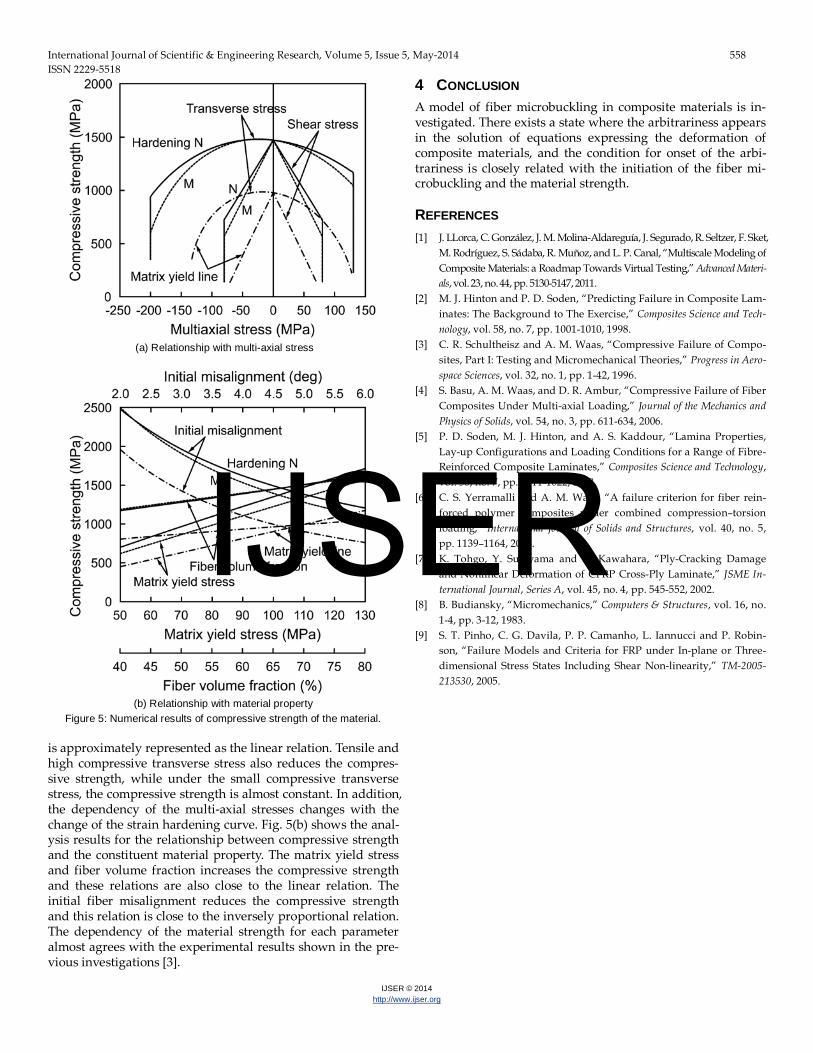
Fig. 5(a) shows the analysis results for the relationship be-tween compressive strength and the multi-axial stresses. The shear stress reduces the compressive strength and this relation

IJSER




is approximately represented as the linear relation. Tensile and high compressive transverse stress also reduces the compres-sive strength, while under the small compressive transverse stress, the compressive strength is almost constant. In addition, the dependency of the multi-axial stresses changes with the change of the strain hardening curve. Fig. 5(b) shows the anal-ysis results for the relationship between compressive strength and the constituent material property. The matrix yield stress and fiber volume fraction increases the compressive strength and these relations are also close to the linear relation. The initial fiber misalignment reduces the compressive strength and this relation is close to the inversely proportional relation. The dependency of the material strength for each parameter almost agrees with the experimental results shown in the pre-vious investigations [3].

4 CONCLUSION A model of fiber microbuckling in composite materials is in-vestigated. There exists a state where the arbitrariness appears in the solution of equations expressing the deformation of composite materials, and the condition for onset of the arbi-trariness is closely related with the initiation of the fiber mi-crobuckling and the material strength.

REFERENCES [1] J. LLorca, C. González, J. M. Molina-Aldareguía, J. Segurado, R. Seltzer, F. Sket,

M. Rodríguez, S. Sádaba, R. Muñoz, and L. P. Canal, “Multiscale Modeling of Composite Materials: a Roadmap Towards Virtual Testing,” Advanced Materi-als, vol. 23, no. 44, pp. 5130-5147, 2011.

[2] M. J. Hinton and P. D. Soden, “Predicting Failure in Composite Lam-inates: The Background to The Exercise,” Composites Science and Tech-nology, vol. 58, no. 7, pp. 1001-1010, 1998.

[3] C. R. Schultheisz and A. M. Waas, “Compressive Failure of Compo-sites, Part I: Testing and Micromechanical Theories,” Progress in Aero-space Sciences, vol. 32, no. 1, pp. 1-42, 1996.

[4] S. Basu, A. M. Waas, and D. R. Ambur, “Compressive Failure of Fiber Composites Under Multi-axial Loading,” Journal of the Mechanics and Physics of Solids, vol. 54, no. 3, pp. 611-634, 2006.

[5] P. D. Soden, M. J. Hinton, and A. S. Kaddour, “Lamina Properties, Lay-up Configurations and Loading Conditions for a Range of Fibre-Reinforced Composite Laminates,” Composites Science and Technology, vol. 58, no. 7, pp. 1011-1022, 1998.

[6] C. S. Yerramalli and A. M. Waas, “A failure criterion for fiber rein-forced polymer composites under combined compression–torsion loading,” International Journal of Solids and Structures, vol. 40, no. 5, pp. 1139–1164, 2003.

[7] K. Tohgo, Y. Sugiyama and K. Kawahara, “Ply-Cracking Damage and Nonlinear Deformation of CFRP Cross-Ply Laminate,” JSME In-ternational Journal, Series A, vol. 45, no. 4, pp. 545-552, 2002.

[8] B. Budiansky, “Micromechanics,” Computers & Structures, vol. 16, no. 1-4, pp. 3-12, 1983.

[9] S. T. Pinho, C. G. Davila, P. P. Camanho, L. Iannucci and P. Robin-son, “Failure Models and Criteria for FRP under In-plane or Three-dimensional Stress States Including Shear Non-linearity,” TM-2005-213530, 2005.

(b) Relationship with material property Figure 5: Numerical results of compressive strength of the material.

(a) Relationship with multi-axial stress

IJSER


1 introduction ijser · takeaki nadabe, nobuo takeda abstract — in this study, a model of fiber...

Documents