A Geometric Approach

to Color Image Regularization

F. Astrom and C. Schnorr

Abstract

We present a new vectorial total variation method that addresses the problem of color consistentimage filtering. Our approach is inspired from the double-opponent cell representation in thehuman visual cortex. Existing methods of vectorial total variation regularizers have insufficient(or no) coupling between the color channels and thus may introduce color artifacts. We addressthis problem by introducing a novel coupling between the color channels related to a pullback-metric from the opponent space to the data (RGB color) space. Our energy is a non-convex,non-smooth higher-order vectorial total variation approach and promotes color consistent imagefiltering via a coupling term. For a convex variant, we show well-posedness and existence of asolution in the space of vectorial bounded variation. For the higher-order scheme we employ ahalf-quadratic strategy, which model the non-convex energy terms as the infimum of a sequenceof quadratic functions. In experiments, we elaborate on traditional image restoration applicationsof inpainting, deblurring and denoising. Regarding the latter, we demonstrate state of the artrestoration quality with respect to structure coherence and color consistency.

CONTENTS

1 Introduction 21.1 Motivation . . . . . . . . . . . . . . . . . . . . . . . . . . . . . . . . . . . . . . . . . . . 21.2 Organization . . . . . . . . . . . . . . . . . . . . . . . . . . . . . . . . . . . . . . . . . . 4

2 Further Related Work 42.1 Color and vector-valued TV . . . . . . . . . . . . . . . . . . . . . . . . . . . . . . . . . . 5

3 Color 73.1 Terminology . . . . . . . . . . . . . . . . . . . . . . . . . . . . . . . . . . . . . . . . . . . 73.2 Color space design . . . . . . . . . . . . . . . . . . . . . . . . . . . . . . . . . . . . . . . 73.3 Double-opponent color representation . . . . . . . . . . . . . . . . . . . . . . . . . . . . 8

4 Geometry of the double-opponent space 94.1 Double-Opponent Metric Tensor . . . . . . . . . . . . . . . . . . . . . . . . . . . . . . . 94.2 Encoded information . . . . . . . . . . . . . . . . . . . . . . . . . . . . . . . . . . . . . . 10

5 General Variational Formulation 115.1 Energy . . . . . . . . . . . . . . . . . . . . . . . . . . . . . . . . . . . . . . . . . . . . . . 115.2 Half-quadratic formulation . . . . . . . . . . . . . . . . . . . . . . . . . . . . . . . . . . . 135.3 First-Order VTV . . . . . . . . . . . . . . . . . . . . . . . . . . . . . . . . . . . . . . . . 16

Date: May 20, 2016Keywords: image analysis, color image restoration, vectorial total variation, double-opponent space, split bregman,

non-convex regularization(F. Astrom) Heidelberg Collaboratory for Image Processing, Heidelberg University, Germany(C. Schnorr) Image and Pattern Analysis Group, Heidelberg University, GermanySupport by the German Research Foundation (DFG) is gratefully acknowledged, grant GRK 1653.

1

arX

iv:1

605.

0597

7v1

[cs

.CV

] 1

9 M

ay 2

016

1 INTRODUCTION 2

6 Implementation and Optimization 176.1 TV and Convex Programming . . . . . . . . . . . . . . . . . . . . . . . . . . . . . . . . . 176.2 Optimization via Split-Bregman and HQA . . . . . . . . . . . . . . . . . . . . . . . . . . 17

7 Applications 197.1 Synthetic image, convergence rate . . . . . . . . . . . . . . . . . . . . . . . . . . . . . . 197.2 Denoising of natural images . . . . . . . . . . . . . . . . . . . . . . . . . . . . . . . . . . 20

7.2.1 Results . . . . . . . . . . . . . . . . . . . . . . . . . . . . . . . . . . . . . . . . . 217.3 Image inpainting, image deblurring . . . . . . . . . . . . . . . . . . . . . . . . . . . . . . 24

8 Discussion and Conclusion 24

References 25

1 INTRODUCTION

1.1 MOTIVATION

Image filtering is a fundamental operation in image processing applications. Typically image filteringrefers to all type of algorithms that modify image pixels in a linear or non-linear manner. Commonapplictions are image denoising (or smoothing) [37, 43, 52, 63, 3, 9, 55], active contours [41], imagedeblurring [50, 16], inpainting [5, 18] and optical flow [35]. These applications have in common thatthey can be formulated as variational problems and are thus inherently related.

In a discrete setting, the solution of such functionals (or energies), can be formulated as maximuma-posteriori (MAP) problems based on markov random fields (MRF), we refer to [66] and [40] for suchapproaches. However, the size of the required label space makes the optimization problem intractableas there is one label for each possible state. Due to this drawback, one computes approximate solutions,e.g., via α-expansion or other relaxation techniques of the label space. The advantage of structuredenergy minimization, such as the MRFs formulation, is that complex neighborhoods, non-smooth andnon-convex penalty functions are easily modelled.

On the other hand, continuous models do not suffer from large label spaces, see for example therecently introduced assignment filter [2]. However, the corresponding optimization problem needs toexplicitly cope with non-smoothness and non-convexity. Convex optimization techniques are well es-tablished methods that efficiently find optimal solutions of convex functions. During the past years, theimaging community has seen a surge of non-convex and often non-smooth energies, often demonstratingimproved results over convex counterparts. The optimization of non-convex functions is particularlychallenging since straightforward approaches often leads to locally optimal solution only.

Relaxation of the non-smooth problems often include modification of the objective function andapproximating non-convex penalty terms via auxiliary variables. Cohen proposed fitting of auxiliaryvariables [22]. However, this approach relies on conjugate functions and if no closed form-solutions areavailable the relaxation method is inefficient. Another popular approach in image processing is thehalf-quadratic algorithm (HQA) introduced by Geman and Reynolds [31]. The HQA approximates anon-convex function as the infimum of quadratic functions as illustrated in Figure 1.1 (a), (b). Onemay also consider lagged fix-point formulations [20]. In this case regularity is imposed via mollificationthat yields a differentiable energy. Subsequently one needs to prove that there exists a convergentfixed-point algorithm.

This work builds on the convex total variation (TV) presented in the seminal work of Rudin, Osherand Fatemi [56]. The success story of total variation (TV) began in 1992 when Rudin, Osher andFatemi [56] introduced an extension of Rudin’s PhD thesis [57]. In Rudin’s work it was conjecturedthat the `1 norm is more appropriate as a regularizer for image processing applications than, e.g., `2norm. The popularity of TV is mainly due to its discontinuity preserving properties, i.e., the norm isa strong prior for avoiding mode mixing and can be interpreted as a the solution of a MAP problem.The common goal for noise reduction methods is to preserve characteristic image features, thus TVis a suitable prior as it is edge preserving. Features of interest vary depending on application area.

1 INTRODUCTION 3

(a) Example of different values of the p-norm forp ∈ (0, 2).

(b) The non-convex energy realized as the infi-mum of quadratic functions (here p = 0.5).

(c) Introduction of artificial colors are shownby the smooth transition from red to green inthe right figure. These types of artifacts oftenarise in image smoothing due to insufficient colorchannel coupling and the denoising scheme’s lackof adaptivity to the image structure.

(d) Example of color shimmering artifacts(right) which often appear in homogeneous im-age regions. Color shimmering can often be sup-pressed with stronger smoothing, however, fre-quently at the cost of oversmoothing image fea-tures (corners/lines etc).

Figure 1.1: Figure (a) shows several instances of the non-convex `p-norm for different p values and (b)shows example HQA approximation for p = 0.5. Figures (c) and (d) illustrates common color imagedenoising artifacts.

However, in general one wishes to preserve structures defining dominant orientations and discontinuitypoints, such as edge and corners, since much of the visual information is contained in contour anddifferences of contrast [54]. Extensions of the initial gray-scale TV prior for image enhancement tocolor images faces the problem to characterize notions of color. The problem of consistent color imageprocessing is largely unsolved and still no consensus on suitable characterization of a “color edge”, ora “color boundary” for general imaging problems has been reached.

This work studies the problem of color image regularization. Extending the scalar TV to colorimages is a non-trivial problem. For example, if a color edge is insufficiently preserved in the smoothingprocess, artificial colors may emerge at the smooth transition between these colors as demonstratedby Figure 1.1 (c). The same figure (d) illustrates the problem of color shimmering, i.e., insufficientsmoothing of homogeneous regions. To address these problems we examine a color space representation,commonly used in computer vision applications and derive a novel color mixing term that penalizesinter-channel discontinuities. We investigate a special instance of color space representation knownas the double-opponent color space. The key aspect of our framework builds on the observation thatthe Jacobian carries vital information useful for color boundary detection. Utilizing this information,we design a TV-based regularizer that describes the color information in a subspace defined by thehue and saturation of the original image color space. Via a higher-order non-convex, non-smoothenergy formulation we show improved discontinuity preserving properties over convex counter-partswith respect to color consistency and structural coherence.

Our approach is motivated based on results from color perception:

• The connection between experienced visual stimuli and current color space models of the visualcortex is naturally modeled using tools from differential geometry. Accordingly, we adopt ageometric viewpoint to explore the relation between color edges and the regularizer based on thecolor space geometries. The double-opponent color space is thought to relate neurophysiologicalproperties of color experience to single-opponent and double-opponent cells in the human cortex,see [30, 44, 45, 26] and references therein. There is recent evidence that a large concentrationof double-opponent cells are located in the region V1, the primary part of the visual cortex [23].Double-opponent cells are thought to be orientation-selective with respect to color discrimination

2 FURTHER RELATED WORK 4

and the detection of color boundaries, results made possible by modern functional magneticresonance imaging (fMRI) techniques [23]. We will use this fact in our subsequent analysis tomotivate the introduction of our model.

When formulating image denoising objective functions one often adopts different viewpoints. Thefollowing two major viewpoints motivate our work: namely color perception and color model.

• Color perception. As stated, we formulate the problem of color image denoising from principlesof color perception. The discriminate power of color is one primary feature for object separationand detection. It is often referred to as a highly important features for the visual system andis closely related to the problem of accurate boundary detection [23]. We present a model thatpreserves discontinuities in the color space motivated by a double-opponent transformation. Bypreserving color discontinuities we hypothesize that color borders trigger the activation of thesedouble-opponent cells and thus yields the experience of crisp color borders in the image.

• Color Model. We denote transportation of the visual (RGB) stimuli to the double-opponent cellsin the visual cortex with a mapping. We postulate that, if there exists a spatial relation betweentwo stimuli (e.g., a color difference), then this induces a response in the double-opponent cells inthe form of orientation sensitivity. The motivation is that double-opponent cells act as color edgedetectors, as shown by neurophysical experiments (again we refer to [30, 44, 45, 26]). Thus, weconclude that there exist a color transition function (or gradient) in the double-opponent space.To obtain the mapping we observe that the stimuli in the opponent space, induced by a linearopponent transformation, in fact gives rise to a pullback metric on the RGB-space where thespatial interaction between the double-opponent cells are modeled by the gradient-operator.

1.2 ORGANIZATION

In Section 2 we sketch the framework of total variation and make the difference between our view-pointto established literature in the field. Already here, we must emphasize that much research in colorimage processing is merely a multi-dimensional extension of the original total variation for gray-scaleimages. The differences between our approach and related VTV methods are also detailed in Section 2.In Section 3 we review color space models often adopted in the image processing literature. In the samesection we also introduce the double-opponent transformation. Section 4 serves to derive the connectionbetween the observation (RGB) space and the double-opponent representation, we also derive resultson the encoded information in the metric decomposition and relate these facts to colorfulness. Thegeneral variational problem is defined in Section 5. In the same section we formulate the correspondingHQA formulation and prove that the HQA is a particular instance of a majorize-minimize algorithmfor the general problem. For the particular instance corresponding to the non-relaxed, first order VTVwith a convex dataterm, we rigorously show convexity of the overall problem, that a solution exists andis unique in Section 5.3. Section 6 describes the numerical scheme and Section 7 presents the numericalevaluation with applications in image denoising, inpainting and deblurring. Section 8 concludes thepaper.

Next we review total variation methods and present current generalizations to color image process-ing before we introduce our framework.

2 FURTHER RELATED WORK

In addition to TV, closest to our work is the seminal work of Sapiro and Ringach [58] who firstobserved that the metric tensor eigendecomposition can be used to describe directional change andmagnitude of color images. In this work we extend this reasoning and show that there exists a naturalcolor space representation which leads to a corresponding interpretation of the Sapiro and Ringachapproach. Unlike the Beltrami flow [42] and Sapiro and Ringach, we exploit the inverse rate of changeof the metric tensor’s eigenvalues. This gives us a transformation from the double-opponent space backto the observation space of the image data. We thus obtain an explicit information about the imagechromaticity, and by extension, the color edge information. The detection of edges is a well investigated

2 FURTHER RELATED WORK 5

field of study for gray-scale images and methods include, e.g., the canny edge detector [11], gradientfilters and the structure tensor [29, 7]. These methods work well for monochromatic images (such asgray-scale images) but the extension to multi-dimensional data such as color image data is still an openproblem. One of the first extension of the structure tensor to multi-valued images was proposed by DiZenzo [70], but later it was reported that channel-by-channel denoising is sufficient in the frameworkof partial differential equations, e.g., [68]. Coupling of the color channels were investigated in [64] anddecorrelation approaches to denoising have also been considered see, e.g., [3].

For a gray-scale image u : Ω→ R defined on a domain Ω ⊂ R2, the total variation measure is givenby

TV (u) = sup

∫Ω

udiv (ϕ) dx : ϕ ∈ C1c (Ω,R2), ‖ϕ‖∞ ≤ 1

(2.1)

A function u ∈ L1(Ω) belongs to the space of functions of bounded variation BV (Ω) if

‖u‖BV (Ω) = ‖u‖L1(Ω) + TV (u) <∞. (2.2)

TV (u) given by (2.1) is a support function in the sense of convex analysis. Thus, combining TV (u) withanother (or more) convex functionals enables to apply a wide range of convex programming techniques.An early basic example is [13]. Further common strategies include the primal-dual algorithm [14] andthe Split-Bregman approach [34].

Next, we review generalizations of scalar TV to vector-valued and color images.

2.1 COLOR AND VECTOR-VALUED TV

Let u : Ω→ Rd, u(x) =(u1(x), ..., ud(x)

)>, denote a vector-valued image. Color images are represented

by the three color components red, green and blue, i.e., d = 3. In this section we review some extensionsof total variation to vector-valued and color images categorized in three main tracks: channel-by-channel, spectral approaches and decorrelation approaches. We briefly mention PDE-based models.

Channel-by-channel. The straightforward extension of TV to vector-valued color image regular-ization is to apply (2.1) channel-by-channel. However, as this naive approach neglects any channel-by-channel correlation one of the first extensions was to penalize color edges across channels as suggestedby Blomgren and Chan [8]. They raised several important aspects highlighting the fact that the ex-tension to color is a non-trivial task. First, they argued that the vector-valued TV should not penalizeintensity edges, as there can be a shift in color but not in intensity. Secondly, they advocate thatthe corresponding TV-regularizer should be rotationally invariant in the image space, although this isdisputed in [51]. Blomgren and Chan propose

TVBC(u) =

√√√√ M∑i=1

TV (ui)2, (2.3)

with the TV term under the sum given by (2.1). However, applying this model to the problem ofcolor image denoising has been shown to produce significant color smearing artifacts due to insufficientpreservation of color edges. The reason of this effect is that the model fails to comprehend that thered, green and blue color components are in fact highly correlated. Thus, due to lacking any couplingbetween the color channels, the model produces suboptimal results w.r.t. to color consistency [33].

Bresson and Chan [10] considered a vector-valued extension of the scalar dual TV formulation.Based on work by Chambolle [13] and Fornasier and March [28], Bresson and Chan presented acoherent framework for vectorial total variation with a study of well-posedness. While their formulationgeneralizes Chambolle’s dual of Blomgrens TV semi-norm (2.3), results still exhibit color smearing.

We refer to [25] for an additional discussion on discrete vectorial total variation models. We remarkthat this underlines the complex nature of color image processing and researchers continued to proposealternative total variation color filtering models, as we will discuss below.

Spectral approaches. One of the first vectorial TV (VTV) schemes that explicitly take colorinformation into account, was introduced by Sapiro and Ringach [58]. In an intensity image an edge is

2 FURTHER RELATED WORK 6

localized by changes in the image intensity. The novelty introduced by Sapiro and Ringach is that theyexploited the metric imposed by the first fundamental form on the image domain, which couples theRGB-channel’s derivatives, to indicate the presence of color edges. The resulting functional is givenby

TVS(u) =

∫Ω

√λ+ − λ− dx, (2.4)

where λ+ > λ− ≥ 0 are the eigenvalues of the metric tensor. Goldluecke and Cremers [32] propose avectorial total variation method based on the largest singular value (hence on the spectral norm) ofthe derivative matrix Du,

TVJ(u) =

∫Ω

σ1(Du) dx. (2.5)

TVJ is closely related to TVS with the difference that TVJ sets all singular values (except) the largest tozero. Although TVJ improves the signal-to noise ratio, the visual appearance for the denoised resultscontains considerable color shimmering, visible in homogeneous regions. Thus, despite a couplingbetween the color channels, the approach still may produce color artifacts.

Decorrelation transforms. Regularization via decorrelation transforms was suggested in e.g.,[19]. A more recent approach to incorporating color into a total variation formulation was introducedby Ono and Yamada [51]. They propose a discrete norm incorporating a weight w between the intensityand chroma in the decorrelation transform O (see also (3.1),(3.2) below)

JV TV (u) = ‖D3Ou‖w1 = w‖D1o1‖1 +

∥∥∥∥(D1o2

D1o3

)∥∥∥∥1

(2.6)

where ‖x‖1 =√∑

i x2i . D1 is the derivative matrix for one channel and D3 = diag(D1, D1, D1) the

three channel derivative matrix. The constant w ∈ (0, 1) determines the weighting between the inten-sity and the chromaticity of the color space. A smaller w will penalize the chroma. This formulation,however, does not take into account that the subspace defined as the chroma (o2, o3) is not decorre-lated but actually consists of the components hue and saturation. The framework does not respectthe non-uniformity of the opponent space. As a consequence, direct regularizing on the chroma via anEuclidean distance metric violates the non-Euclidean structure of this opponent space. Furthermore,it is easy to construct scenarios where the image saturation changes independently of the hue, thusfurther motivating why the chroma should be decoupled into hue and saturation [48].

PDE-based models. There are many PDE-based models for color image filtering. We confineourselves to referring to [3, 64, 68] and to discussing the work of Chambolle [12] who proposed a partialdifferential equation (PDE)-based anisotropic diffusion model. This model aims to solve the problemof color constancy (referring to the work by Poggio [36]). Although Chambolle did not present anenergy-based total variation approach, his treatment of the color channels and their smoothing alongthe image gradient direction is relevant to our subsequent analysis. Chambolle defines a PDE withdirectional diffusivity ξ defined as

ξ ⊥(

(u2 − u3)∇u1 + (u3 − u1)∇u2 + (u1 − u2)∇u3

)= 0, (2.7)

reducing smoothing perpendicular to the gradients. The coupling between color channels is explicit:the difference of the intensity level of two color components affects the directional smoothing of thethird channel. In practice, ξ is used in the heat equation to inhibit smoothing close to color edges.However, as noted by Sapiro and Ringach [58], if two channels are equiluminant and if the third channelhas an edge, this edge will remain unaffected by the filter.

Although these ideas were presented more than two decades ago, they did not attract much atten-tion in the image processing community. We will see that our perceptual model is related to (2.7) inthat our approach penalizes the pair-wise differences between the image derivatives, not the pair-wiseintensity differences. In Section 4 we derive a color descriptor which couples the color channels in anatural way derived from the geometry of the double-opponent color transform. We will show that acolor channel coupling similar to that of Chambolle, in combination with related ideas to the geometricframework of Sapiro and Ringach [58], results in a natural description of the image colorfulness.

3 COLOR 7

3 COLOR

Color perception is a well studied area and researchers continue to propose color models. To use the“correct” color model is application dependent and a non-trivial problem. In this work we focus onthe application of denoising. Next we briefly introduce established principles of color space design andrecall some terminology.

3.1 TERMINOLOGY

Some of the earliest works on color theory date back to the work by Newton [49]. In modern sciences,Albert Munsell is often accredited the notion color dimensions hue, value and saturation [48]. Figure3.1 illustrates the dimensions where hue is an angular component, value the intensity and saturationa radial component. For consistent use of the color terminology see The Commission Internationalede l’Eclairage (International Commission on Illumination, CIE) [21] and [60]. For further in-depthinformation on color image processing and the structure of color we refer to [60]. When we writeintensity, we mean lightness, implying the monochromatic component black and its brightness, orsimply, the image gray-scale component. When we write saturation we refer to the magnitude of thecolor vector orthogonal to the lightness, and hue refers to an angle ranging from 0 to 360 degrees asillustrated in Figure 3.1. During the last decades several color systems have been proposed to representcolor, each considering different constraint sets. The next section reviews some of the more frequentlyreferred color space representations.

Figure 3.1: An isoluminant disc of the doule-opponent color space. Hue is an angular componentdescribing the primary colors red, green, blue, and the opponent colors yellow, magenta and cyan andthe corresponding colors transitions. Saturation describes the colorfulness of the corresponding hueand value gives the intensity with which the color is perceived. In the case of scalar valued (gray-scaleimages) the saturation is null and thus the hue plays no role.

3.2 COLOR SPACE DESIGN

It is important to note when dealing with color theory that color is a subjective experience. Infact, one often thinks of color as wavelength of light. This is a misconception, however, since coloris a result of neural processing in the human brain [61, Ch. 4]. This alludes to the difficulty ofobtaining a quantitative and accurate description of color. Next, we list four major points that requireconsideration when determining suitable color space representations.

• Easy to use. Modeling psychophysical effects of color in scientific applications is a highly non-trivial problem. The study of physical stimulus of different wavelengths has shown that thecharacterization of color in the human visual system is dominantly done by, what is accepted asthe colors red, green, blue and yellow. These colors are in fact electromagnetic waves and can berepresented as spectral power distributions (SPD) [60]. This realization of color perception gaverise to one of the earliest color models namely the CIE 1931 XYZ color space which builds onthe trichromatic color representation of red (R), green (G) and blue (B). In modern applicationsthese colors constitute the basis of the RGB color space and is widely used to represent imagecontent. In the RGB color space, the relationship between two colors is linear and this simplifiedrepresentation is also its main drawback. This Euclidean treatment of color relations is notaccurate, in fact, as shown in numerous works (see [60] and references therein), the human

3 COLOR 8

visual system is less sensitive to short wavelenghts (e.g., blue), and this therefore suggests thatthe color spectral distributions should be represented non-uniformly. However, despite obviousoversimplifications in the RGB-representation it may be sufficiently good and easy to use for theconsidered application and thus motivates its use.

• Color reproduction. Color reproduction is the problem of reproducing color independent ofdisplay system. The Munsell system [48], was the first standardization for color metrics widelyaccepted and later adopted by CIE in 1931. The recommendations set forth by CIE still continueto influence today’s color research [60]. Due to the subjective nature of color perception manycolor models have been proposed, however, appropriate color space representation seems so far tobe application dependent and no consensus has been reached. Due to the emerging technology ofInternet and the large variety of imaging display systems and hardware limitations, a standardizedRGB color space called sRGB was proposed for consistent image rendering over a wide rangeof devices [62]. Even up to present time, sRGB is a widely used color space on the world wideweb. Also CIELAB is used for color reproduction due to its perceptual uniform structure and ismentioned next.

• Perceptual uniformity. The CIELAB color space was developed for perceptual uniformity.Color and perceptual uniformity, for image processing applications, implies that a perturbationin, e.g., hue, may influence a reference color to a different degree and may induce color artifactsfor certain colors, but not for others. Perceptually, this is known to as the just-noticeable-difference and can be visualized via MacAdam ellipses [47]. In reality it has been shown thatthe CIELAB is almost perceptually uniform, see [60] and references therein. This motivates theuse of non-Euclidean metrics, even in supposedly perceptually uniform cases, to determine thedistance between colors. Due to the strong emphasis on perceptual uniformity the CIELAB colorspace is less suitable for rigorous mathematical treatment due to numerous discontinuities it itsdefinition.

• Hardware limitations. Many color spaces were introduced as a consequence of technical andhardware limitations. Such a color space was the HSV (Hue, Saturation, Value) color space devel-oped in the 1970 for applications related to color display systems [38]. The YCbCr/YPbPr colorspaces were proposed for analog and digital television transmission, respectively. Furthermore,the YCbCr/YPbPr signal representation include non-linear mappings and chroma bandlimitingfunction to enable efficient transmission of the image signal [53]. One can also argue that thepreviously mentioned sRGB is part of this category. Due to the strong adaptation to efficient en-gineering requirements, color spaces in this category have not been subject to extensive researchin the context of color image processing.

Next we present the double-opponent color space.

3.3 DOUBLE-OPPONENT COLOR REPRESENTATION

Recall that the most commonly used color space is the RGB color space. It consists of three compo-nents, r, g and b which are the Red, Green and Blue components. These components are uniformlyspaced in [0, 255] (or [0, 1]) depending on the chosen quantization. The r, g, b components are highlycorrelated, and thus image processing algorithms without explicit color adaptation introduce artifi-cial colors and color smearing. To address this problem, a decorrelation transform is usually applied,converting the color space into the three components of lightness, saturation and hue1.

The mapping from the decorrelated double-opponent space in the visual cortex to a physical stimuliis denoted via a function ψ−1 : R3 → R3 defined by (3.3) below. We denote by, u : Ω→ R3, the physicalstimuli containing red, green and blue spectra. Furthermore, denote by the linear mapping

O : R3 → R3, u = (r, g, b)> 7→ Ou = o = (o1, o2, o3)>, (3.1)

1The transformation to these components is not equivalent with the HSV color space. Although, the interpretationof the components are similar.

4 GEOMETRY OF THE DOUBLE-OPPONENT SPACE 9

the transformation from the RGB color space to the double-opponent space where the matrix O isdefined as (see [30, 44, 45, 26, 46]),

O =

1/√

3 0 0

0 1/√

6 0

0 0 1/√

2

1 1 11 1 −21 −1 0

. (3.2)

We note that this linear mapping has full rank. The matrix O actually describes a rotation and scalingof the RGB coordinate system. The opponent component o1 is nothing else than the gray-scale value,o2 is the subtraction of yellow (mixing red and green equals yellow) from blue and the last componento3 is the subtraction of green from red, i.e., o2 and o3 consists of the opponent colors in the RGB colorspace.

The non-linear mapping to the hue (h), saturation (s) and lightness (L) representation of thedecorrelated double-opponent space is given by

ψ : R3 → R3, o 7→ c = (L, h, s)> (3.3)

where

L = o1, h = arctan

(o2

o3

), s =

∥∥∥∥(o2

o3

)∥∥∥∥ , (3.4)

Let ϕ : R3 → R3 denote the composition of the linear opponent transform (3.2) and the mapping(o1, o2, o3)> 7→ (L, h, s)> just discussed above, then we define

ϕ : u→ ϕ(u) := ψ(Ou). (3.5)

In the next section we compute the metric tensor associated with the mapping ϕ and investigates itsencoded information.

4 GEOMETRY OF THE DOUBLE-OPPONENT SPACE

In this section we derive a color representation that allows for an intuitive interpretation of the double-opponent color space as components of the RGB-space. Subsequently we give an exposition on theinformation that this representation’s encodes.

4.1 DOUBLE-OPPONENT METRIC TENSOR

Strictly speaking, in this work, we regard the RGB-space as a linear Riemannian manifoldM equippedwith the metric (4.1), which is an inner product on the tangent space TuM that smoothly varies withu ∈ M. Since every tangent space TuM can be identified with M, however, it makes sense to regardthe Riemannian metric (4.1) as inner product defined on the space itself. We refer, e.g., to [39] forbackground and further details.

The Euclidean inner product 〈·, ·〉 on the Lhs-space induces via ϕ the pullback metric on theRGB-space which is given by

〈u1, u2〉u := 〈Dϕ(u)u1, Dϕ(u)u2〉 = 〈u1, G(u)u2〉, (4.1a)

G(u) :=(Dϕ(u)

)>Dϕ(u) =

(gij(u)

)i,j=1,2,3

. (4.1b)

One identifies that

u = (u1, u2, u3)> = (r, g, b)>, (4.2a)

α = α(u) := (α1, α2, α3)> = (b− g, r − b, g − r)>, (4.2b)

β = β(u) := (β1, β2, β3)>

= (b+ g − 2r, b+ r − 2g, r + g − 2b)>, (4.2c)

f2 = f2(u) := ‖α‖2

= 2(b2 − bg − br + g2 − gr + r2). (4.2d)

4 GEOMETRY OF THE DOUBLE-OPPONENT SPACE 10

In the subsequent analysis we return to the following decomposition

γ = f2 = u>Pu P =

2 −1 −1−1 2 −1−1 −1 2

0. (4.3)

where P is a symmetric and positive semi-definite matrix. Furthermore, one easily verifies the relations

α ⊥ β, u ⊥ α, α× β = f21, (4.4a)

〈u, β〉 = f2, ‖β‖2 = 3‖α‖2. (4.4b)

The Jacobian Dϕ and the corresponding metric tensor G read

Dϕ(u) =1√3

(1,

3

f

α

‖α‖,

1

fβ

)>, (4.5a)

G(u) =1

3

(I +

9

f4αα> +

1

f2ββ>

), (4.5b)

where G has non-normalized eigenvectors 1, α, β and corresponding eigenvalues

Λ =1

3I + diag

(0,

3

f2, 1

). (4.6)

Saprio and Ringach [58] also exploited the first fundamental form but in Euclidean space and concludedthat the tensor’s eigenvalues capture the color edge information. Here we instead use the principaldirectional change obtained from the eigendecomposition of the double-opponent metric tensor. Andour focus is on γ of (4.3) (which is f2). Similarly to Saprio and Ringach, the interpretation is that alarge eigenvalue of the tensor will indicate the presence of image color. Next, we justify and elaboratethis statement in the next section while investigating the information encoded in γ.

4.2 ENCODED INFORMATION

This section investigates the information encoded in the metric tensor, decomposed into an eigensystemas in the previous section. The derived γ describes the colorfulness of an image, and in the next sectionwe formulate an energy model that explicitly preserve discontinuities in γ. We identify the followingrelation

γ(u) = u>Pu = (b− r)2 + (r − g)2 + (g − b)2

= ‖u>C1‖2, C1 =

1 −1 00 1 −1−1 0 1

. (4.7)

Note that P = C1C1> (cmp. (4.3)). The coefficients of C1u have previously appeared in an early work

by Chambolle [12].

Proposition 4.1. The function, γ in (4.7), has the properties (P1) γ(u+c1) = γ(u) and (P2) γ(cu) =c2γ(u), where c is a constant.

Proof. The result follows immediately from (4.7).

The above result yields the following interpretation of the γ-function: a) (P1) shows that γ isinvariant to intensity shifts. b) (P2) shows that γ has a quadratic dependency on intensity changes. c)It follows from a) that γ depends on color changes. d) It follows from b) that γ depends on color shifts.Under constant intensity, γ captures change of color as illustrated by Figure 4.1 (a), (b). In this figurewe show equiluminant discs at constant intensity along with the corresponding response of γ. It isclearly visible that γ describes the intrinsic color structure of the color space as there is a stronger

5 GENERAL VARIATIONAL FORMULATION 11

(a)

(b)(c)

Figure 4.1: (a) Color discs with corresponding response of γ, (4.7), in (b). The largest magnitude(red color) is obtained at the primary colors (red, green and blue) and the opponent colors (yellow,cyan and magenta). As expected, the response on the intensity axis (center of discs) is 0 (black). (c)Interpretation of the vector r − g as an orthogonal component to yellow.

response for highly saturated colors. In the lower half of the intensity range we predominantly detectthe primary colors red, green and blue. As the intensity increases, γ shows primary responses fromyellow, cyan and magenta. The intensity axis is located in the center of these discs and, as expected,we do not obtain a value of colorfulness. We give some examples of γ-responses from natural imagesin Figure 5.1.

The geometric interpretation of γ is illustrated as an example via the r− g-component. The othertwo color difference terms follow with similar reasoning. We know that the color yellow, y, is composedas a sum of red and green, i.e., y = r + g, and written in vector form we have r − g = (1,−1, 0)> andy = r+ g = (1, 1, 0)>. We see that yellow is perpendicular to the difference r− g, i.e., y ⊥ (r− g) = 0.This is illustrated in Figure 4.1 (c). Analogous argument hold for the other terms of γ, i.e., b − r isorthogonal to magenta, and g−b orthogonal to cyan. In this way γ covers the RGB space. Moreover, asγ describes the color structure, preserving its edge information prevents color distortion in the filteringprocess. Based on this analysis, we are now prepared to introduce the general variational formulation.

5 GENERAL VARIATIONAL FORMULATION

Let u = [u>R, u>G, u

>B ]> ∈ R3N (Ω) represent a color image on the domain Ω with stacked color channels.

N is the number of pixels in one image channel. Also, let g ∈ R3N be the corresponding noisy data.

We define the discrete image gradient for one channel as D1 =

[Dx

Dy

]∈ R2N×N , Dx, Dy ∈ RN×N and

subscript denotes the forward finite difference operator in x and y directions, respectively. Furthermore,we let i ∈ N+ s.t. Ii ∈ Ri×i denotes the identity matrix. In this notation, the three channel derivativematrix for a color image is D(1) = D1 ⊗ I3 ∈ R6N×3N where ⊗ is the Kronecker product and

D(1)u : R3N → R6N (5.1)

is the derivative matrix for the three channels.

5.1 ENERGY

Channel-by-channel filtering of the RGB space is prone to introduce color artifacts [8, 10]. On the otherhand, purely decorrelating the color channels without considering the geometry is also sub-optimal, seeresults in, e.g., [58, 51]. We propose a two-component regularizer: one component performs channel-by-channel filtering penalizing all intra-channel content and one component which explicitly targets thecolor information. The color specific prior defines a natural inter-channel coupling from the geometry

5 GENERAL VARIATIONAL FORMULATION 12

Figure 5.1: Detected color structure in real images extracted by γ. In these examples, primary colorssuch as red, green and blue and the opponent color yellow are well characterized.

of the double-opponent space, realized through

C ∈ R3N×3N , C = C1 ⊗ IN (5.2)

where C1 corresponds to (4.7).For M ∈ N let m ∈ 1, ..,M, then we define α, β ∈ RM+ and p, q ∈ RM (0, 2), such that α, β, p, q

are vectors with components indexed by subscript, e.g., αm. We let s ∈ (0, 2) and by ‖x‖pp we mean

‖x‖pp =

3N∑i=1

|xi|p. (5.3)

The energy we introduce and study in this work is defined as the non-convex optimization problem

minu

E(u) = 1

s‖Ku− g‖ss

+∑Mm=1

(αm

pm‖D(m)u‖pmpm + βm

qm‖D(m)Cu‖qmqm

), (5.4)

where D(m) is the m-order derivative matrix. When m = 1 we have a first-order energy and if m = 2,we have a second-order energy and so forth. To be explicit, we give the derivative matrix for the firstand second order cases

D(1) =

(Dx

Dy

)(5.5a)

and

D(2) =

Dxx

Dxy

Dyx

Dyy

(5.5b)

where subscript denotes the derivative in x and y-directions, respectively. The operator K ∈ R3N×3N

in (5.4) is the identity matrix in the case of denoising or a blurring matrix in the case of deconvolution.Since the product Cu is now the pair-wise mixture of color channels, it means that DCu is the pair-wise mixture of the channel gradients, i.e., DCu penalizes color opponent gradients in y, c and m, andDu penalizes the primary colors r, g and b. With m > 1 we have a natural definition of higher-ordertotal variation. Although C is a constant matrix, it is non-trivial to minimize E due to its inherentnon-convexity when either of p, q, s ∈ (0, 1). For this reason, we adopt a half-quadratic formulationpresented next.

5 GENERAL VARIATIONAL FORMULATION 13

5.2 HALF-QUADRATIC FORMULATION

Alternatives to the HQA [31] include, e.g., fitting of auxiliary variables [22] which, however for practicalapplications, relies on the efficient evaluation of a conjugate function. One may also consider lagged fix-point formulations [20], in this case one would impose regularity to obtain a differentiable energy andprove that there exists a convergent fixed-point algorithm. Instead, the HQA algorithm is particularlysuited to optimize E since we obtain a computationally very efficient scheme. Furthermore, identifyingthat the HQA can be written as an instance of a majorize-minimize scheme we also show that theHQA convergences to a stationary point corresponding to a minimum. We make use of the followingresult to optimize our energy

Lemma 5.1. (HQA p-norm [15]) Let p ∈ (0, 2) and t ∈ (R \ 0), then

‖t‖p = minv>0

vt2 +

1

ξvγ

(5.6)

where γ = p2−p , ξ = 22/(2−p)

(2−p)pp/(2−p) , and the minimum is obtained at

v∗ =p

2|t|p−2. (5.7)

The energy E in (5.4) is not differentiable and not convex. To apply the HQA, we make use of the

mollified energy Eε and set ‖x‖ηη,ε =∑Mi=1(|xi| + ε)η =

∑Mi |xi|ηε and 0 < η < 2. Now, the energy

Eε(u) is differentiable but not convex, therefore the direct optimization problem

uk+1 = minuEε(u) (5.8)

may result in a locally optimal solution. The HQA optimization problem takes the form

minu

Eε(u) =

3N∑i=1

1

sminz>0

(zi|Kiu− gi|2ε +

1

ξszαsi

)

+

M∑m=1

[αmpm

minvm>0

(vi,m|D(m)

i u|2ε +1

ξpmvαpmi,m

)

+βmqm

minwm>0

(wi,m|D(m)

i Cu|2ε +1

ξqmwαqmi,m

)](5.9a)

=: minu,v1>0,...,vm>0,w1>0,...,wm>0,z>0

L(u, v, w, z) (5.9b)

now convex separately in u and in z, v, w, respectively. We use subscript “i” to denote the i’th row (orcomponent) of a matrix (or vector). By using Lemma 5.1 we formulate an alternating minimizationstrategy where the update equations for the auxiliary variables are given by

zk+1 =s

2|Kuk − g|s−2

ε (5.10a)

(vk+1m , wk+1

m ) =

pm2|D(m)uk|pm−2

εqm2|D(m)Quk|qm−2

ε

> , m = 1, ...,M (5.10b)

and the norm is taken component-wise. The update equation for the convex subproblem uk+1 isobtained by minimizing

uk+1 = arg minu

3N∑i=1

1

szk+1i |Kiu− g|2ε

+

M∑m=1

(αmpm

vk+1i,m |D

(m)i u|2ε +

βmqm

wk+1i,m |D

(m)i Cu|2ε

)(5.11)

5 GENERAL VARIATIONAL FORMULATION 14

Convergence analysis. The main idea of the following convergence result is to express the HQAas an instance of the majorize-minimize (MMA) algorithm [20]. Once we establish the link betweenthe HQA and the MMA we can show convergence of our algorithm.

Assume there exists a function Φ such that

minuEε(u) = min

uΦ(u) (5.12)

and to show that the HQA formulation is of the MMA-type we consider the optimization problem

uk+1 = arg minuF(u, uk). (5.13)

If there exists a function Φ such that F satisfies

F(u, uk) ≥ Φ(u), for ∀u ∈ Rn (5.14a)

F(u, uk) = Φ(u), for u = uk (5.14b)

∇uF(u, uk) = ∇Φ(u), for u = uk (5.14c)

With L from (5.9b) and taking into account that vk+1, wk+1, zk+1 depend on uk, we define:

F(u, uk) := L(u, vk+1, wk+1, zk+1) (5.15)

and have the following result

Proposition 5.2 (MMA). The optimization problem (5.11), stemming from the HQA, is an instanceof MMA with F defined as in (5.15).

Proof. We adopt a the solution strategy introduced in [15]. The first step is to start by substitute(5.10) into (5.15) and get expression (5.16). Then we set F(u = uk, uk) which results in

F(uk, uk) =

3N∑i=1

1

2|Kiu

k − gi|sε

+

M∑m=1

(αm|D(m)

i uk|pmε + βm|D(m)i Cuk|qmε

)= Φ(uk) (5.17)

where Φ was defined in (5.12) and establishes condition (5.14b). In order to show condition (5.14a),i.e., that F forms an upper envelope of Φ(u) we identify that (5.16) can be expressed with Young’sinequality. Then under the condition 1/a+ 1/b = 1 we have that

ga

a+hb

b≥ gh. (5.18)

We set ξ(u) = |Kiu− gi|ε

g = ξ(uk)(s−2)s

2 ξ(u)s (5.19a)

h = ξ(uk)(2−s)s

2 (5.19b)

F(u, uk) =

3N∑i=1

1

s

(s

2|Kiu

k − gi|s−2ε |Kiu− gi|2ε +

(2− s)2|Kiu

k − gi|sε)

+

M∑m=1

[αmpm

(pm2|D(m)

i uk|p−2ε |D(m)

i u|2ε +(2− pm)

2|D(m)

i uk|pmε)

+βmqm

(qm2|D(m)

i Cuk|qm−2ε |D(m)

i Cu|2ε +(2− qm)

2|D(m)

i Cuk|qmε)]

(5.16)

5 GENERAL VARIATIONAL FORMULATION 15

and let a = 2s , b = 2

2−s , which verifies the inequality

s

2|Kiu

k − gi|s−2ε |Kiu− gi|2ε +

(2− s)2|Kiu

k − gi|sε≥ |Kiu− gi|sε, i = 1, ..., 3N (5.20)

With an analogous reasoning of the remainder of (5.16) components we have that F(u, uk) ≥ Φ(u),i.e., condition (5.14a) is fulfilled. Finally, one easily verifies that ∇uF(u, uk) = ∇Φ(u) at u = uk, thus(5.14c) holds. This shows that F(u, uk) is a majorizing function of (5.9).

Theorem 5.3 (Convergence). Given a sequence uk generated by HQA, then (i) Φ(uk), (5.17), ismonotonically decreasing and convergent and (ii) lim ‖uk − uk+1‖22 = 0 as k →∞.

Proof. The first and second order derivatives of F are

∇uF(u, uk) =

3N∑i=1

1

szk+1i K>i (Kiu− gi)

+

M∑m=1

2αmpm

vk+1i,m (D(m))>i D

(m)i u

+ 2βmqm

wk+1i,m (D

(m)i Q)>D

(m)i Qu (5.21)

and

∇2uF(u, uk) =

1

s

3N∑i=1

zk+1i K>i Ki

+

M∑m=1

2αmpm

vk+1i,m (D(m))>D(m)

+ 2βmqm

wk+1i,m (D(m)Q)>D(m)Q (5.22)

where the latter matrix is positive semidefinite independently of u. Thus, F is convex in u. Moreover,by (5.13) and (5.14),

Φ(uk+1) ≤ F(uk+1, uk) ≤ F(uk, uk) = Φ(uk). (5.23)

From this it is immediate thatlimk→∞

Φ(uk)− Φ(uk+1) = 0 (5.24)

as Φ is bounded from below by 0. To show the convergence of uk, we consider the Taylor expansionof F(u, uk) at uk+1

F(u, uk) = F(uk+1, uk)

+1

2(u− uk+1)∇2F(u, uk)(u− uk+1) (5.25)

where the first-order term on the right-hand side vanishes due to the optimality condition of (5.13).

Note that higher-order differentials ∇(n)u F , n > 2 vanish. Minimizing the right-hand side with respect

to u and then setting u = uk, we obtain

F(uk, uk) ≥ F(uk+1, uk) +ξ

2‖uk − uk+1‖22 (5.26)

where ξ is positive and is the minimum eigenvalue of ∇2uF . Consequently,

F(uk, uk)−F(uk+1, uk) ≥ ξ

2‖uk − uk+1‖22 ≥ 0, (5.27)

with the left-hand side converging to 0 due to (5.23) and (5.24).

5 GENERAL VARIATIONAL FORMULATION 16

Based on the identification with a MMA, we have shown convergence and existence of a solution forthe corresponding HQA. Although, this result is significant, we required a mollifier, a constant offset εin the denominator. This parameter regularizes the energy and thus introduces smoothness, albeightbeing small, an returns a smoother solution than desired. In the numerical evaluation we implementthe above energy with an iterative Split-Bregman scheme and we obtain stable updates for ε as smallas 10−20, which we also used in the numerical evaluation. Next, we study the natural selection offirst order derivative (m = 1), quadratic data term (s = 2) and corresponding vectorial total variationregularization (p, q = 1) with the same channel coupling matrix as in the HQA. In this case we do notrequire a mollification and we show that the corresponding minimizer resides in the space of vectorialbounded variation and is unique.

5.3 FIRST-ORDER VTV

As a special instance of the general variational formulation (5.4) we study the existence of a solutionof a non-mollified vectorial total variation term. Consequently we are not required to use the HQA.In this section we will also use a continuous formulation which is more efficient for this purpose, assuch, we use the coupling matrix C1 ∈ R3×3 defined in (4.7).

In the following, let ∇u = (∇u1,∇u2,∇u3) : Ω→ R2×3 be the vectorial gradient of an color imagein the generalized sense as discussed in connection with eq. (2.1), Then we define p = (p1, p2, p3) ∈C1c (Ω; R2×3) with Div (p) = (div (p1) ,div (p2) ,div (p3))>.

Definition 5.1 (Double-opponent VTV). The double opponent regularizer is defined as

JOPP (u) :=

∫Ω

‖∇C1u‖ (5.28a)

:= sup‖p‖∞≤1

∫Ω

〈C1u,Div (p)〉 dx

(5.28b)

where ‖p‖∞ = max‖p1‖, ‖p2‖, ‖p3‖.

Next, we show that the regularizer JOPP is convex, invariant to rotation and intensity shift of thecolor space.

Theorem 5.4 (Invariance and convexity). JOPP is rotationally and intensity invariant, 1-homogeneousand convex.

Proof. Rotational invariance follows from the isotropy of the feasible set of the dual variable p, thatis ‖p‖∞ = ‖(p1, p2, p3)‖∞ ≤ 1 =⇒ ‖(Rp1, Rp2, Rp3)‖∞ ≤ 1, for any orthogonal matrix R. As aconsequence of property (P1) and (P2) of Prop. 4.1, JOPP is invariant to intensity shifts, and therelation JOPP (cu) = cJOPP (u) is immediate, for any positive constant c > 0. Finally, convexityfollows from the definition of JOPP as pointwise supremum of affine functions.

The non-mollified first-order energy of (5.4), with a convex dataterm, is defined as

minu

E(u) =µ

2‖Ku− g‖2L2(Ω)

+α∑3i=1 TV(ui) + βJOPP (u)

(5.29)

where µ, α, β > 0.

Existence of solution. Next we show that the variational approach (5.29) is well posed.

Lemma 5.5 (Bounded variation). Let u ∈ BV (Ω; R3) then C1u ∈ BV (Ω; R3).

Proof. Transposing the matrix C1 in the integrand of (5.28b) shows that JOPP (u) is the supportfunction of u with respect to the image of the unit ball p : ‖p‖∞ ≤ 1 under the linear mappingC>1 Div. The claim then follows from the assumption u ∈ BV (Ω; R3).

6 IMPLEMENTATION AND OPTIMIZATION 17

As a consequence, the objective function E(u) (5.29) is well defined. We next show that there is aunique color image u minimizing E(u).

Theorem 5.6 (Uniqueness and existence of solution). Let g ∈ L∞(Ω,R3) and u ∈ BV (Ω,R3). Thenthere exists a unique minimizer u∗ of E(u) given by (5.29).

Proof. We adapt and sketch a standard proof pattern from [4]. Due to g ∈ L∞(Ω,RM ), we may assumethat all admissible u are uniformly bounded in the sense that |ui(x)| ≤ ‖gi‖L∞(Ω), i = 1, 2, 3, ∀x ∈ Ω.Let (un)n∈N be a minimizing sequence with respect to E(u). Then, after passing to a subsequence(unk

)k∈N, there exists a u∗ ∈ BV (Ω; R3) with unk→ u∗ strongly in L1

loc(Ω; R3), ∇(ui)nk→ ∇u∗i in

an appropriate weak sense, and Jopp(unk) → Jopp(u

∗) in view of Lemma 5.5. It follows from Fatou’slemma and the lower-semicontinuity of E(u) that u∗ minimizes E(u), whereas uniqueness of u∗ is aconsequence of the strict convexity of E(u) due to the data term of (5.29).

Next, we derive an efficient numerical scheme which optimizes our proposed energies.

6 IMPLEMENTATION AND OPTIMIZATION

We briefly comment on convex programming techniques that are relevant to our approach. Thenwe detail our implementation of a specific technique embedded into the half-quadratic regularizationapproach.

6.1 TV AND CONVEX PROGRAMMING

There exists numerous methods to minimize the total variation semi-norm. A very popular approachis the primal-dual iteration from Chambolle and Pock [17, 14]. Related algorithms include the splitbregman method [34], augmented Lagrangian methods [69] and the alternating direction method ofmultipliers (ADMM) [65]. The split-Bregman technique has been shown to be equivalent to ADMMin the case of a linear constraint set [27]. Further connections between these methods are discussed in[69].

An evaluation of these algorithms in connection with our approach is beyond the scope of thispaper. We adopted the split-Bregman algorithm [34] as an established technique and incorporatedit as subroutine of our half-quadratic regularization approach, without claiming that this is the bestpossible choice.

6.2 OPTIMIZATION VIA SPLIT-BREGMAN AND HQA

With the notation introduced in Section 5 above, and with the discretized channel matrix C ∈ R3N×3N

(see (5.2)) we write the discretized form of (5.4) as the optimization problem

minu,d,e

µ

2‖Ku− g‖22 +

M∑m=1

(α‖dm‖pp + β‖em‖qq

)(6.1a)

s.t. dm = D(m)u, em = D(m)Cu. (6.1b)

Let ‖v‖2H := 〈v,Hv〉 be a weighted Euclidean norm and d = (d>1 , ..., d>m)>, e = (e>1 , ..., e

>m)>. Let

D = (vec(D(1))>, ..., vec(D(m))>)> (6.2)

(cf. (5.5)) and set

B(u, b, d, e) :=

(de

)−(DDC

)u− b. (6.3)

6 IMPLEMENTATION AND OPTIMIZATION 18

Applying the Split Bregman approach yields the iteration

(uk+1, dk+1, ek+1) = minu,d,e

µ

2‖Ku− g‖22

+ ‖d‖pp + ‖e‖qq +1

2‖B(u, b, d, e)‖2H , (6.4a)

bk+1 = bk +

(DDC

)uk+1 −

(dk+1

ek+1

). (6.4b)

In the cases of p = 1 and/or q = 1 we apply the shrinkage operator to minimize d, e, respectively.When p, q are in the non-convex range (0, 1), we use the HQA in Lemma 5.1 and obtain the point-wisequadratic update step

(dk+1, ek+1) = mind,e

vk+1d2 + wk+1e2

+1

2

∥∥B(uk+1, bk, d, e)∥∥2

H, (6.5a)

(vk+1, wk+1) =(p

2|dk|p−2

ε ,q

2|ek|q−2

ε

), (6.5b)

which is strictly convex in both d and e. Since (6.5) is defined point-wise, we get the optimalitycondition,

2

(vk+1dwk+1e

)+

(α 00 β

)((de

)−(DDC

)uk − b

)= 0 (6.6)

and the closed-form update-expression(dk+1

ek+1

)=

((Duk + b1)/(1 + 2vk+1/α)

(DCuk + b2)/(1 + 2wk+1/β)

). (6.7)

The optimization problem w.r.t. u is solved iteratively by

uk+1 = minu

µ

2‖Ku− g‖22 +

1

2

∥∥B(u, bk, dk, ek)∥∥2

H. (6.8)

In (6.8), we set b = [b>1 , b>2 ]> for notational convenience and compute

µK>(Kuk+1 − g)− αD>(dk −Duk+1 − bk1

)− β(DC)>

(ek −DCuk+1 − bk2

)= 0 (6.9)

which gives the update step(µK>K + αD>D + β(DC)>(DC)

)uk+1

= µK>g + αD>(dk − bk1) + β(DC)>(ek − bk2). (6.10)

Our experiments confirm the observation of [34] that only computing an approximate solution ac-celerates the overall iterative scheme without compromising convergence. Consequently, we merelyapply few conjugate gradient iterative steps to compute uk+1. This is computationally cheap since allmatrices involved are sparse.

Finally, we iterate the steps (6.10), (6.5b), (6.7) and (6.4b) until we satisfy the stopping criterion

‖uk − uk+1‖22/‖uk+1‖22 < 0.9√

3Nσ2/2552, (6.11)

where σ is the noise level standard deviation. This numerical scheme gives stable updates even whenε is very small. In the experimental evaluation we fixed ε = 10−20.

7 APPLICATIONS 19

Iteration

20 40 60 80

Error

0.02

0.04

0.06

0.08

0.1

Iteration

20 40 60 80

PSNR

26

28

30

32

34

36

38

(a) Normalized difference between two consecu-tive updates in the iterative update (6.10) com-puted as (6.11).

(b) PSNR value of the current iterate uk. Thesecond order VTV (m = 2) consistently resultsin improved PSNR values.

Figure 7.1: Empirical convergence (a) of the image data in figure 7.2. The numerical scheme isimplemented as presented in Section 6 and the trend of the corresponding PSNR curves are shown in(b). The regularization parameters were set as µ = 80, α1 = β1 = 2 for first order VTV. In the secondorder case we additionally set α2 = β2 = 1.

(a) Original (b) Noisy (c) First order VTV (d) Second order VTV

Figure 7.2: Synthetic isoluminant test image (a) which consists of affine regions that compose slantingplanes in the color space, transitioning from blue to green. (b) shows the noisy data. (c) and (d) depictthe first and second order VTV when p = 0.6. This image illustrates that there is (i) no introductionof artificial colors and (ii) quality of reconstruction is more smooth in the second order VTV comparedto the first order VTV due to the higher order constraints on jump-transitions in the image data. Yetthe second order VTV shows good edge preservation. The empirical convergence and PSNR valuesare shown in figure 7.1 (a) and (b).

7 APPLICATIONS

We apply our approach to color image denoising, inpainting and deblurring. All images were normalizedto the range [0, 1] given in an 8-bit representation. In addition to a qualitative evaluation we includethe measures peak signal-to-noise ratio (PSNR), the structural similarity index (SSIM) [67] and theCIEDE 2000 which is a measure of color consistency [59]. We consider two denoising scenarios. Onesynthetic case where the image data consist of piecewise affine regions. The other scenario concernsthe denoising of natural images.

7.1 SYNTHETIC IMAGE, CONVERGENCE RATE

The synthetic image is isoluminant and therefore presents a particular challenge due to the absenceof gray-scale edges. Figure 7.1 shows the empirical convergence rate of our approach for first (m = 1)and second (m = 2) order VTV for the noisy image in Figure 7.2. For each parameter setting thesecond order VTV shows improved PSNR values which correlates with the visual impression of thefinal result images in Figure 7.2 (c) and (d), respectively.

7 APPLICATIONS 20

7.2 DENOISING OF NATURAL IMAGES

The aim of this section is to illustrate differences between commonly benchmarked methods. With thisin mind we evaluate the performance of the proposed energy and optimize each method with respectto its parameters and noise levels. The following methods and parameter ranges are included in theevaluation and we refer to the respective works for further details:

• Decorrelated VTV [51] (DVTV): Search space for optimal parameter configuration is τ ∈0.95, 1, 1.05, w ∈ 0.3, 0.4, 0.5, 0.6, 0.7.

• Primal-dual VTV [10] (PDVTV): The regularization parameter was optimized for 5 uniformlysampled values in the range 10−3 to 0.2.

• Total generalized variation [9] (TGV): Applied component-wise and only included for compari-son. The regularization parameter was uniformly sampled with 5 values in the range 10−3 and0.25.

• Color BM3D [24] (BM3D): The standard deviation of the additive Gaussian noise was given asinput.

We evaluate our double-opponent (OPP) formulation, see (5.4) for the case of a first (OPP1p) and

second order energy OPP2p. We restrict q = p and let p ∈ 0.2, 0.6, 0.8, 1. The following parameter

setup was used:

• (OPP1p): First-order scheme optimized with µ ∈ 10, 20, 30, 40, 80, 100 and fixed α1 = β1 = 2.

• (OPP2p): Second-order scheme optimized with µ ∈ 10, 20, 30, 40, 80, 100 and α1 = β1 = 2 and

α2 = β2 = 1.

• (OPP11): Optimized parameter space of µ are 5 uniformly sampled values from 1/255 to 30/255,

α = 1 and β was uniformly sampled in from 5 values in the range 1/255 to 5/255.

The experimental evaluation use 100 color images from the Weizmann Institute [1]. The imagedata were normalized to the range [0, 1] using a 8-bit representation.

We are interested in consistent color image processing, that is we are specifically tackling the colorimage filtering problem. Accordingly, we consider the case that the color of the image is corruptedby additive Gaussian noise, not the intensity channel. Until now this denoising setup has not beenbenchmarked and poses an interesting task, i.e., the recovery of color information. Rather thancorrupting all image data with additive noise, we corrupt the components (o2 and o3) with 20, 40, 60or 80 standard deviations of Gaussian noise and ignore the intensity channel.

After transforming from the (now noisy) opponent representation to the RGB space, one can showthat the r,g,b components retain a Gaussian noise distribution as the following calculation illustrates.Let σ2

i , i = 1, 2, 3 denote the standard deviation of zero mean Gaussian noise, then the opponent com-ponents, now seen as random variables, are normally distributed, i.e., oi ∼ N (0, σ2

i ). Transformationfrom the double-opponent space to the RGB color space is done via

u = O−1o, O−1 =

1/√

3 1/√

6 1/√

2

1/√

3 1/√

6 −1/√

2

1/√

3 −2/√

6 0

. (7.1)

Assuming normally distributed opponent components o ∼ N (0,Σo), Σo = Diag(0, σ2, σ2), we obtainu ∼ N (0,Σu) with

Σu = O−1ΣoO−T (7.2)

Excluding the inter-channel correlation between the r,g,b components in (7.2) the noise transformationis given by

u ∼ N (0,2

3Diag(σ2, σ2, σ2)). (7.3)

Therefore, we also evaluate BM3D with a scaled standard deviation. We denote this approach as

• Scaled-BM3D (BM3DS): Color BM3D with√

2/3 of the noise standard deviation.

Next we present and discuss the results obtained with OPP and the compared methods.

7 APPLICATIONS 21

Original Noisy (60)15.0/0.35/23.40

OPP1p OPP2

p OPP11 BM3D [24]

23.3/0.71/8.27 23.8/0.75/8.15 24.3/0.73/6.90 22.6/0.63/6.16

DVTV [51] PDVTV [10] TGV [9] BM3DS [24]18.8/0.37/10.29 21.1/0.57/10.98 21.0/0.57/10.85 23.0/0.64/6.95

Figure 7.3: Visual comparison of the compared methods and corresponding error values. The resultof our OVTV produces the most accurate result, only marginally beaten by BM3D in terms of coloraccuracy. Yet, the visual quality of OVTV is more clear and does not suffer from desaturated colorsas in DVTV.

7.2.1 RESULTS

Table 2 shows the average PSNR, SSIM and CIEDE error measures for each method and noise level.Three methods stand out: OPP1

p, OPP11 and BM3D. For lower noise-levels the non-convex first-order

method OPP1p shows highest PSNR and SSIM values. While OPP1

1 performs marginally better thanOPP1

p for noise levels larger than 60 standard deviations of noise, BM3D has the best CIEDE accuracyfor all noise levels. Comparing only energy based methods (i.e., not BM3D/BM3DS) it is clear thatall OPP-based methods show improved accuracy for PSNR, SSIM and CIEDE in all cases. In all casesOPP2

p shows worse accuracy than OPP1p (except SSIM at noise level 60) due to the extra smoothness

constraints imposed by the higher-order derivative. OPP2p is more suitable for images with piecewise

affine regions, such as illustrated in the synthetic example, Section 7.1.The principal difference between OPP1

1 and PDVTV is that the additional color mixing regular-ization term is included in the former, thus illustrating the success of the mixing term in OPP. Withrespect to error measures we see an improvement in each case for OPP1

1. Comparing the second order

7 APPLICATIONS 22

Noisy OPP1p OPP2

p OPP11

24.6/0.81/9.90 29.5/0.92/4.40 26.1/0.81/4.59 27.9/0.88/4.33

19.0/0.58/17.39 24.4/0.79/7.75 24.6/0.77/6.46 25.3/0.82/6.72

15.8/0.42/22.94 22.0/0.69/10.13 22.3/0.70/9.70 21.7/0.68/10.99

13.6/0.31/27.25 20.2/0.57/9.59 20.3/0.62/12.02 20.5/0.60/10.33

Figure 7.4: Qualitative comparison between OPP. From top row to bottom row the noise levels theimages are corrupted with 20, 40, 60 and 80 standard deviations of noise. For higher noise-levels thesecond-order OPP2

p shows improved SSIM, in particular for noise level 80 shows less oversmoothing ofthe background image structure. Although, it contains more color shimmering reflected in the higherCIEDE value. For lower noise levels, the first-order methods seem preferable. (PSNR/SSIM/CIEDE)

OPP2p with the result of TGV the error value differences are smaller, however OPP still shows improved

results.The visual quality, comparing all methods for the (high) noise level 60, is seen in Figure 7.3.

All methods suffer from color shimmering in homogeneous regions, although, the shimmering is lessobvious for BM3D, which also shows the best color consistency. Although, the result of BM3D isheavily oversmoothed, seen in the detailed panel and the trees in the background. All versions of theproposed OPP show higher PSNR and SSIM, although in these examples, there is color shimmering.DVTV shows the worst performance and shows strong structural oversmoothing of the trees in thebackground and there is strong evidence of color smearing. We remark that DVTV is designed for thecolor transform used in this work, however the method is fundamentally different from ours: DVTV

7 APPLICATIONS 23

Original Noisy15.6/0.28/18.71

OPP1p OPP2

p OPP11

23.3/0.71/6.02 23.7/0.73/5.55 24.1/0.74/5.21

Figure 7.5: Example result images from the evaluation dataset for 60 standard deviations of Gaussiannoise. In this image the OPP1

1 performs shows marginally better performance than the non-convexcounter-parts. (PSNR/SSIM/CIEDE)

considers the intensity and the color information as orthogonal and independent, and also regularizethese separately, however, for the color image data, this is not the case in practice and the methodfails as this assumption is violated.

Figure 7.4 shows the output for the OPP methods for different noise levels. At the lowest noise-level, the result images appears crisp and do not contain disturbing color artifacts at color edges.Color shimmering artifacts are naturally more pronounced as the noise level increases, due to im-precise parameter settings. Hand-tuning regularization parameters to separate image structure fromnoise increase clarity and suppress color shimmering, however, further accurate determination of theseparameters is subject to further study.

To additionally illustrate the recovery of noisy images using OPP, Figures 7.5 and 7.6 show twochallenging images at noise level 60 standard deviations of Gaussian noise. Figure 7.5 is an imagewith vivid colors and many details, visually each methods performs well. OPP1

1 appear most crisp andproduces the most smooth background whereas OPP1,2

p both preserve the flower well. Figure 7.6 showssimilar characteristics as the previous example, although in this case OPP2

p shows a larger degree ofcolor shimmering than OPP1

p and OPP11. Each of the methods does compensate for the image noise

well and preserves facial-features and the stamp’s text.Table 1 shows the average error for the used p-values in the evaluation of the 100 natural images.

There is an indication towards better performance for PSNR and SSIM for p in the range 0.6-0.9whereas CIEDE suggests smaller p-values for the first order scheme. Error values for the second orderscheme is in general worse than the first order, this is due to the additional smoothness introduced bythe higher-order derivatives. However, as seen in the synthetic result in Section 7.1, the second-orderscheme performs very well when the image data is mostly affine.

8 DISCUSSION AND CONCLUSION 24

Original Noisy15.8/0.17/22.44

OPP1p OPP2

p OPP11

24.9/0.64/5.17 25.1/0.65/5.65 25.1/0.63/5.27

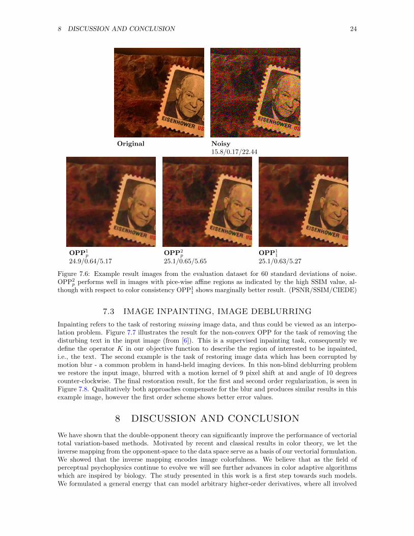
Figure 7.6: Example result images from the evaluation dataset for 60 standard deviations of noise.OPP2

p performs well in images with pice-wise affine regions as indicated by the high SSIM value, al-though with respect to color consistency OPP1

1 shows marginally better result. (PSNR/SSIM/CIEDE)

7.3 IMAGE INPAINTING, IMAGE DEBLURRING

Inpainting refers to the task of restoring missing image data, and thus could be viewed as an interpo-lation problem. Figure 7.7 illustrates the result for the non-convex OPP for the task of removing thedisturbing text in the input image (from [6]). This is a supervised inpainting task, consequently wedefine the operator K in our objective function to describe the region of interested to be inpainted,i.e., the text. The second example is the task of restoring image data which has been corrupted bymotion blur - a common problem in hand-held imaging devices. In this non-blind deblurring problemwe restore the input image, blurred with a motion kernel of 9 pixel shift at and angle of 10 degreescounter-clockwise. The final restoration result, for the first and second order regularization, is seen inFigure 7.8. Qualitatively both approaches compensate for the blur and produces similar results in thisexample image, however the first order scheme shows better error values.

8 DISCUSSION AND CONCLUSION

We have shown that the double-opponent theory can significantly improve the performance of vectorialtotal variation-based methods. Motivated by recent and classical results in color theory, we let theinverse mapping from the opponent-space to the data space serve as a basis of our vectorial formulation.We showed that the inverse mapping encodes image colorfulness. We believe that as the field ofperceptual psychophysics continue to evolve we will see further advances in color adaptive algorithmswhich are inspired by biology. The study presented in this work is a first step towards such models.We formulated a general energy that can model arbitrary higher-order derivatives, where all involved

REFERENCES 25

Original OPP10.8 OPP2

0.8

Figure 7.7: The input image contains disturbing text as shown in red color. The restoration task is toremove this text. Final results for the second and first order VTV formulations are seen on the secondrow for p = 0.8. Both approaches produces convincing results without introducing disturbing colorartifacts or oversmoothing.

Input OPP10.8 OPP2

0.8 (PSNR/SSIM/CIEDE)

24.20/0.73/3.84 32.27/0.93/1.94 30.76/0.92/2.01

Figure 7.8: Example of image sharpening with known motion blur. This example shows that both ourfirst and second order VTV formulations produce high-quality results without introducing disturbingcolor artifacts, oversmoothing homogeneous regions or over sharpening artifacts.

regularization terms can be convex, non-convex or a mixture. Automatic parameter selection foroptimal restoration performance remains an open problem. We discretizised and decomposed ourformulation using the iterative split Bregman scheme, and we demonstrated competitive performancecompared to standard vectorial total variation methods and state of the art denoising algorithmsevaluated using commonly used error measures in the image restoration community.

REFERENCES

[1] Alpert, S., Galun, M., Basri, R., Brandt, A.: Image Segmentation by Probabilistic Bottom-UpAggregation and Cue Integration. In: Proceedings of the IEEE Conference on Computer Visionand Pattern Recognition (June 2007)

[2] Astrom, F., Petra, S., Schmitzer, B., Schnorr, C.: Image Labeling by Assignment. pre-print,http://arxiv.org/abs/1603.05285 (2016)

[3] Astrom, F., Baravdish, G., Felsberg, M.: On Tensor-Based PDEs and their Corresponding Vari-ational Formulations with Application to Color Image Denoising. In: ECCV 2012: 12th Euro-pean Conference on Computer Vision, 7-12 October, Firenze, Italy. LNCS, vol. 7574. SpringerBerlin/Heidelberg (2012)

REFERENCES 26

OPP1p OPP2

p

PSNR/p 0.3 0.6 0.9 0.3 0.6 0.9

20 32.4 ± 2.3 32.9 ± 2.0 33.0 ± 1.7 29.6 ± 3.4 30.0 ± 3.2 31.1 ± 2.740 27.5 ± 2.5 28.1 ± 2.4 28.4 ± 1.9 28.0 ± 2.4 28.0 ± 2.2 28.2 ± 1.960 24.5 ± 2.3 25.3 ± 2.0 25.5 ± 2.1 25.6 ± 1.9 25.6 ± 1.8 25.4 ± 1.980 22.7 ± 2.2 23.3 ± 2.1 23.4 ± 1.8 23.3 ± 1.9 23.3 ± 1.8 23.2 ± 1.9

SSIM

20 0.90 ± 0.05 0.91 ± 0.05 0.91 ± 0.04 0.82 ± 0.09 0.84 ± 0.07 0.88 ± 0.0540 0.79 ± 0.08 0.81 ± 0.08 0.83 ± 0.07 0.80 ± 0.08 0.81 ± 0.07 0.82 ± 0.0660 0.69 ± 0.11 0.74 ± 0.09 0.75 ± 0.09 0.75 ± 0.08 0.75 ± 0.08 0.75 ± 0.0880 0.63 ± 0.13 0.68 ± 0.11 0.69 ± 0.09 0.68 ± 0.10 0.69 ± 0.09 0.69 ± 0.09

CIEDE

20 2.99 ± 2.64 2.97 ± 2.63 3.04 ± 2.64 3.42 ± 2.66 3.34 ± 2.63 3.23 ± 2.6240 4.51 ± 2.54 4.40 ± 2.53 4.46 ± 2.55 4.61 ± 2.51 4.69 ± 2.52 4.73 ± 2.5560 5.84 ± 2.48 5.64 ± 2.42 5.68 ± 2.42 5.86 ± 2.41 5.93 ± 2.43 5.95 ± 2.4480 6.90 ± 2.31 6.81 ± 2.28 6.91 ± 2.28 7.09 ± 2.30 7.13 ± 2.31 7.14 ± 2.32

Table 1: Error measures and standard deviation for the first and second-order OPP for varying p-values. These values were obtained in the optimization of the 100 images in the natural image denoisingevaluation. Table 2 shows the best obtained results in this evaluation scenario.

[4] Attouch, H., Buttazzo, G., Michaille, G.: Variational Analysis in Sovolev and BV Spaces: Apli-cations to PDEs and Optimization. SIAM, 2nd edn. (2014)

[5] Ballester, C., Bertalmio, M., Caselles, V., Sapiro, G., Verdera, J.: Filling-in by joint interpolationof vector fields and gray levels. Image Processing, IEEE Transactions on 10(8), 1200–1211 (2001)

[6] Bertalmio, M., Sapiro, G., Caselles, V., Ballester, C.: Image inpainting. In: Proceedings of the27th Annual Conference on Computer Graphics and Interactive Techniques. pp. 417–424. SIG-GRAPH ’00, New York, NY, USA (2000)

[7] Bigun, J., Granlund, G.H.: Optimal Orientation Detection of Linear Symmetry. In: Proceedingsof the IEEE First International Conference on Computer Vision. pp. 433–438 (1987)

[8] Blomgren, P., Chan, T.: Color TV: total variation methods for restoration of vector-valued images.Image Processing, IEEE Transactions on 7(3), 304–309 (Mar 1998)

[9] Bredies, K., Kunisch, K., Pock, T.: Total generalized variation. SIAM Journal on Imaging Sciences3(3), 492–526 (2010)

[10] Bresson, X., Chan, T.: Fast dual minimization of the vectorial total variation norm and applica-tions to color image processing. Inverse Problems and Imaging 2(4), 455–484 (Nov 2008)

[11] Canny, J.: A computational approach to edge detection. Pattern Analysis and Machine Intelli-gence, IEEE Transactions on PAMI-8(6), 679–698 (Nov 1986)

[12] Chambolle, A.: Partial differential equations and image processing. In: Image Processing, 1994.Proceedings. ICIP-94., IEEE International Conference. vol. 1, pp. 16–20 vol.1 (Nov 1994)

[13] Chambolle, A.: An Algorithm for Total Variation Minimization and Applications. Journal ofMathematical Imaging and Vision 20(1-2), 89–97 (2004)

[14] Chambolle, A., Pock, T.: A First-Order Primal-Dual Algorithm for Convex Problems with Ap-plications to Imaging. Journal of Mathematical Imaging and Vision 40(1), 120–145 (2011)

REFERENCES 27

OPP

1 pOPP

2 pOPP

1 1PDVTV

[10]

DVTV

[51]

TGV

[9]

BM

3D

[24]

BM

3DS

[24]

σ=

20

PS

NR

33.1

±1.85

31.1

±2.7

232.0

±2.1

029.8

±2.0

427.0

±0.9

927.3

±2.7

432.9

±2.0

032.6

±1.1

9S

SIM

0.92

±0.04

0.8

8±

0.0

50.8

9±

0.0

50.8

5±

0.0

50.7

9±

0.0

80.7

8±

0.0

80.9

0±

0.0

50.8

7±

0.0

5C

IED

E3.3

7±

2.7

03.3

1±

2.6

62.8

6±

2.6

84.7

5±

2.9

14.5

7±

2.4

85.4

4±

4.1

52.78

±2.66

3.6

3±

2.6

4σ

=40

PS

NR

28.4

±2.0

628.2

±1.9

828.4

±1.93

25.9

±2.1

622.8

±2.1

725.4

±2.5

828.0

±2.6

127.5

±1.7

5S

SIM

0.83

±0.07

0.8

2±

0.0

70.8

2±

0.0

70.7

3±

0.0

80.6

0±

0.1

40.7

1±

0.0

90.7

9±

0.0

90.7

4±

0.0

7C

IED

E5.0

3±

2.6

95.3

3±

2.6

55.1

6±

2.8

36.7

8±

3.0

67.1

2±

2.5

06.6

8±

3.6

04.31

±2.57

5.6

1±

2.6

0σ

=60

PS

NR

25.5

±2.0

725.5

±1.8

225.9

±1.84

23.5

±1.6

621.9

±2.2

123.6

±2.0

525.2

±2.5

825.1

±2.0

7S

SIM

0.7

5±

0.0

80.76

±0.07

0.7

6±

0.0

90.6

0±

0.0

50.5

7±

0.1

60.6

5±

0.1

00.7

1±

0.1

20.6

8±

0.0

9C

IED

E6.4

6±

2.8

86.9

3±

2.7

46.0

6±

2.5

79.2

2±

2.7

67.7

3±

2.5

28.2

1±

3.1

75.32

±2.46

6.2

3±

2.4

6σ

=80

PS

NR

23.4

±1.9

323.2

±1.8

223.5

±1.82

20.9

±1.0

121.0

±2.0

421.9

±2.0

023.2

±2.3

723.2

±2.1

1S

SIM

0.70

±0.09

0.6

9±

0.0

90.7

0±

0.0

90.4

5±

0.0

60.5

5±

0.1

60.6

0±

0.1

10.6

6±

0.1

40.6

4±

0.1

2C

IED

E7.6

0±

2.6

48.3

0±

2.8

57.9

2±

2.7

812.7

5±

2.4

08.3

1±

2.3

99.5

8±

3.4

66.39

±2.34

7.0

1±

2.2

9

Tab

le2:

Err

or

mea

sure

sfo

rth

eev

alu

ate

dm

eth

od

s.

REFERENCES 28

[15] Chan, R.H., Liang, H.X.: Half-quadratic algorithm for `p-`q problems with applications to TV-`1image restoration and compressive sensing. In: Bruhn, A., Pock, T., Tai, X.C. (eds.) EfficientAlgorithms for Global Optimization Methods in Computer Vision, LNCS, vol. 8293, pp. 78–103.Springer Berlin Heidelberg (2014)

[16] Chan, T., Wong, C.K.: Total variation blind deconvolution. Image Processing, IEEE Transactionson 7(3), 370–375 (1998)

[17] Chan, T.F., Golub, G.H., Mulet, P.: A nonlinear primal-dual method for total variation-basedimage restoration. SIAM Journal on Scientific Computing 20(6), 1964–1977 (1999)

[18] Chan, T.F., Kang, S.H., Kang, Shen, J.: Euler’s elastica and curvature based inpaintings. SIAMJ. Appl. Math 63, 564–592 (2002)

[19] Chan, T.F., Kang, S.H., Shen, J.: Total Variation Denoising and Enhancement of Color ImagesBased on the CB and HSV Color Models. Journal of Visual Communication and Image Repre-sentation 12(4), 422 – 435 (2001)

[20] Chan, T.F., Mulet, P.: On the convergence of the lagged diffusivity fixed point method in totalvariation image restoration. SIAM Journal on Numerical Analysis 36(2), 354–367 (1999)

[21] CIE: International lighting vocabulary. CIE Publ, Vienna 4(17) (1987)

[22] Cohen, L.D.: Auxiliary Variables and Two-step Iterative Algorithms in Computer Vision Prob-lems. J. Math. Imaging Vis. 6(1), 59–83 (1996)

[23] Conway, B.R., Chatterjee, S., Field, G.D., Horwitz, G.D., Johnson, E.N., Koida, K., Mancuso,K.: Advances in color science: From retina to behavior. J. Neurosci. 30(45), 14955–14963 (2010)

[24] Dabov, K., Foi, A., Katkovnik, V., Egiazarian, K.: Color Image Denoising via Sparse 3D Col-laborative Filtering with Grouping Constraint in Luminance-Chrominance Space. In: Image Pro-cessing, 2007. ICIP 2007. IEEE International Conference on. vol. 1, pp. I – 313–I – 316 (Sept2007)

[25] Duran, J., Moeller, M., Sbert, C., Cremers, D.: Collaborative Total Variation: A General Frame-work for Vectorial TV Models (2015), http://arxiv.org/abs/1508.01308

[26] Ebner, M.: Color Constancy. Wiley Publishing, 1st edn. (2007)

[27] Esser, E.: Applications of lagrangian-based alternating direction methods and connections to splitbregman. In: UCLA, Technical Report 09-31, Computational and Applied Mathematics (2009)

[28] Fornasier, M., March, R.: Restoration of color images by vector valued bv functions and variationalcalculus. SIAM Journal on Applied Mathematics 68(2), 437–460 (2007)

[29] Forstner, W., Gulch, E.: A fast operator for detection and precise location of distinct points,corners and centres of circular features. In: ISPRS Intercommission, Workshop, Interlaken, pp.149-155. (1987)

[30] Gao, S., Yang, K., Li, C., Li, Y.: A color constancy model with double-opponency mechanisms.In: Computer Vision (ICCV). pp. 929–936 (Dec 2013)

[31] Geman, D., Yang, C.: Nonlinear image recovery with half-quadratic regularization. Image Pro-cessing, IEEE Transactions on 4(7), 932–946 (1995)

[32] Goldluecke, B., Cremers, D.: An approach to vectorial total variation based on geometric measuretheory. In: Computer Vision and Pattern Recognition (CVPR), 2010 IEEE Conference on. pp.327–333 (2010)

[33] Goldluecke, B., Strekalovskiy, E., Cremers, D.: The natural vectorial total variation which arisesfrom geometric measure theory. SIAM Journal on Imaging Sciences 5(2), 537–563 (2012)

REFERENCES 29

[34] Goldstein, T., Osher, S.: The Split Bregman Method for L1-Regularized Problems. SIAM Journalon Imaging Sciences 2(2), 323–343 (2009)

[35] Horn, B.K.P., Schunck, B.G.: Determining optical flow. ARTIFICAL INTELLIGENCE 17, 185–203 (1981)

[36] Hurlbert, A., Poggio, T.: Synthesizing a color algorithm from examples. Science 239, 182–485(1998)

[37] Iijima, T.: Basic theory of pattern observation. In: Papers of Technical Group on Automata andAutomatic Control, IECE, Japan (1959)

[38] Joblove, G.H., Greenberg, D.: Color spaces for computer graphics. In: Proceedings of the 5thAnnual Conference on Computer Graphics and Interactive Techniques. pp. 20–25. SIGGRAPH’78, ACM, New York, NY, USA (1978)

[39] Jost, J.: Riemannian Geometry and Geometric Analysis. Springer, 4th edn. (2005)

[40] Kappes, J., Andres, B., Hamprecht, F., Schnorr, C., Nowozin, S., Batra, D., Kim, S., Kausler,B., Kroger, T., Lellmann, J., Komodakis, N., Savchynskyy, B., Rother, C.: A ComparativeStudy of Modern Inference Techniques for Structured Discrete Energy Minimization Problems.Int. J. Comp. Vision 115(2), 155–184 (2015)

[41] Kass, M., Witkin, A., Terzopoulos, D.: Snakes: Active contour models. International Journal ofComputer Vision 1(4), 321–331 (1988)

[42] Kimmel, R., Malladi, R., Sochen, N.: Images as Embedded Maps and Minimal Surfaces: Movies,Color, Texture, and Volumetric Medical Images. International Journal of Computer Vision 39(2),111–129 (2000)

[43] Koenderink, J.J.: The Structure of Images. Biological Cybernetics 370(50), 363–370 (1984)

[44] Land, E.: Recent advances in retinex theory and some implications for cortical computations:color vision and the natural image. Proc Natl Acad Sci USA 80(16), 5163–5169 (1983)

[45] Land, E.: An alternative technique for the computation of the designator in the retinex theory ofcolor vision. Proc Natl Acad Sci USA 83(10), 3078–3080 (1986)

[46] Lenz, R., Latorre Carmona, P.: Hierarchical s(3)-coding of rgb histograms. In: Ranchordas, A.,Pereira, J., Arajo, H., Tavares, J. (eds.) Computer Vision, Imaging and Computer Graphics.Theory and Applications, Communications in Computer and Information Science, vol. 68, pp.188–200. Springer Berlin Heidelberg (2010)

[47] MacAdam, D.L.: Visual sensitivities to color differences in daylight. J. Opt. Soc. Am. 32(5),247–273 (May 1942)

[48] Munsell, A.: A Color Notation. G. H. Ellis Company (1905)

[49] Newton, I.: New theory about light and colors. Philosophical Transactions 6(69-80), 3075–3087(1671)

[50] Oliveira, J.P., Bioucas-Dias, J.M., Figueiredo, M.A.: Adaptive Total Variation Image Deblurring:A Majorization-Minimization Approach. Signal Processing 89(9), 1683 – 1693 (2009)

[51] Ono, S., Yamada, I.: Decorrelated Vectorial Total Variation. In: Computer Vision and PatternRecognition (CVPR), 2014 IEEE Conference on. pp. 4090–4097 (2014)

[52] Perona, P., Malik, J., Pietro, P.: Scale-space and edge detection using anisotropic diffusion. IEEEtransactions on Pattern Analysis and Machine Intelligence 12(7), 629–639 (Jul 1990)

REFERENCES 30

[53] Poynton, C.: 24 - luma and color differences. In: Poynton, C. (ed.) Digital Video and HDTV,pp. 281 – 300. The Morgan Kaufmann Series in Computer Graphics, Morgan Kaufmann, SanFrancisco (2003)

[54] Ratliff, F.: Contour and contrast. Proceedings of the American Philosophical Society 115(2), pp.150–163 (1971)

[55] Roth, S., Black, M.J.: Fields of experts: a framework for learning image priors. In: ComputerVision and Pattern Recognition, 2005. CVPR 2005. IEEE Computer Society Conference on. vol. 2,pp. 860–867 vol. 2 (June 2005)

[56] Rudin, L.I., Osher, S., Fatemi, E.: Nonlinear Total Variation Based Noise Removal Algorithms.Phys. D 60(1-4), 259–268 (Nov 1992)

[57] Rudin, L.I.: Images, Numerical Analysis of Singularities and Shock Filters. Ph.D. thesis, CaliforniaInstitute of Technology, California Institute of Technology (1987)

[58] Sapiro, G., Ringach, D.: Anisotropic diffusion of multivalued images with applications to colorfiltering. Image Processing, IEEE Transactions on 5(11), 1582–1586 (Nov 1996)

[59] Sharma, G., Wu, W., Dalal, E.N.: The CIEDE2000 color-difference formula: implementationnotes, supplementary test data, and mathematical observations. Color research and application30(1), 21–30 (2005)

[60] Sharma, G.: Digital Color Imaging Handbook. CRC Press, Inc., Boca Raton, FL, USA (2002)

[61] Shevell, S.K.: The science of color. Optical Society of America, 2003. (2003)

[62] sRGB: Multimedia systems and equipment - Colour measurement and management - Part 2-1:Colour management - Default RGB colour space - sRGB. IEC 61966-2-1 (1999-10), ICS codes:33.160.60, 37.080 - TC 100 - 51 pp. as amended by Amendment A1:2003 (2003)

[63] Tomasi, C., Manduchi, R.: Bilateral filtering for gray and color images. In: Computer Vision,1998. Sixth International Conference on. pp. 839–846 (Jan 1998)

[64] Tschumperle, D., Deriche, R.: Vector-valued image regularization with pde’s: A common frame-work for different applications. In: Proceedings of the 2003 IEEE Computer Society Conferenceon Computer Vision and Pattern Recognition. pp. 651–656. CVPR’03, IEEE Computer Society,Washington, DC, USA (2003)

[65] Wahlberg, B., Boyd, S., Annergren, M., Wang, Y.: An admm algorithm for a class of totalvariation regularized estimation problems. In: Preprints of the 16th IFAC Symposium on SystemIdentification. pp. 83–88 (2012)

[66] Wang, C., Komodakis, N., Paragios, N.: Markov Random Field modeling, inference & learning incomputer vision & image understanding: A survey. Computer Vision and Image Understanding117(11), 1610–1627 (2013), http://dx.doi.org/10.1016/j.cviu.2013.07.004

[67] Wang, Z., Bovik, A., Sheikh, H., Simoncelli, E.: Image quality assessment: from error visibilityto structural similarity. Image Processing, IEEE Transactions on 13(4), 600–612 (April 2004)

[68] Weickert, J.: Coherence-enhancing diffusion filtering. International Journal of Computer Vision31(2-3), 111–127 (1999)

[69] Wu, C., Tai, X.C.: Augmented Lagrangian Method, Dual Methods, and Split Bregman Iterationfor ROF, Vectorial TV, and High Order Models. SIAM J. Img. Sci. 3(3), 300–339 (Jul 2010)

[70] Zenzo, S.D.: A note on the gradient of a multi-image. Computer Vision, Graphics, and ImageProcessing 33(1), 116 – 125 (1986)