In Neil Salkind (Ed.), Encyclopedia of Research Design.

Thousand Oaks, CA: Sage. 2010

Matrix Algebra

Herve Abdi ⋅ Lynne J. Williams

1 Introduction

Sylvester developed the modern concept of matrices in the 19th cen-tury. For him a matrix was an array of numbers. Sylvester workedwith systems of linear equations and matrices provided a convenientway of working with their coefficients, so matrix algebra was to gen-eralize number operations to matrices. Nowadays, matrix algebra isused in all branches of mathematics and the sciences and constitutesthe basis of most statistical procedures.

2 Matrices: Definition

A matrix is a set of numbers arranged in a table. For example, Toto,Marius, and Olivette are looking at their possessions, and they arecounting how many balls, cars, coins, and novels they each possess.Toto has 2 balls, 5 cars, 10 coins, and 20 novels. Marius has 1, 2, 3,

Herve AbdiThe University of Texas at Dallas

Lynne J. WilliamsThe University of Toronto Scarborough

Address correspondence to:Herve AbdiProgram in Cognition and Neurosciences, MS: Gr.4.1,The University of Texas at Dallas,Richardson, TX 75083–0688, USAE-mail: herve@utdallas.edu http://www.utd.edu/∼herve

2 Matrix Algebra

and 4 and Olivette has 6, 1, 3 and 10. These data can be displayedin a table where each row represents a person and each column apossession:

balls cars coins novels

Toto 2 5 10 20Marius 1 2 3 4Olivette 6 1 3 10

We can also say that these data are described by the matrix de-noted A equal to:

A =⎡⎢⎢⎢⎢⎢⎣

2 5 10 201 2 3 46 1 3 10

⎤⎥⎥⎥⎥⎥⎦. (1)

Matrices are denoted by boldface uppercase letters.

To identify a specific element of a matrix, we use its row andcolumn numbers. For example, the cell defined by Row 3 and Column1 contains the value 6. We write that a3,1 = 6. With this notation,elements of a matrix are denoted with the same letter as the matrixbut written in lowercase italic. The first subscript always gives therow number of the element (i.e., 3) and second subscript always givesits column number (i.e., 1).

A generic element of a matrix is identified with indices such as iand j. So, ai,j is the element at the the i-th row and j-th column ofA. The total number of rows and columns is denoted with the sameletters as the indices but in uppercase letters. The matrix A has Irows (here I = 3) and J columns (here J = 4) and it is made of I ×Jelements ai,j (here 3 × 4 = 12). We often use the term dimensions torefer to the number of rows and columns, so A has dimensions I byJ .

ABDI & WILLIAMS 3

As a shortcut, a matrix can be represented by its generic elementwritten in brackets. So, A with I rows and J columns is denoted:

A = [ai,j] =

⎡⎢⎢⎢⎢⎢⎢⎢⎢⎢⎢⎢⎣

a1,1 a1,2 ⋯ a1,j ⋯ a1,Ja2,1 a2,2 ⋯ a2,j ⋯ a2,J⋮ ⋮ ⋱ ⋮ ⋱ ⋮

ai,1 ai,2 ⋯ ai,j ⋯ ai,J⋮ ⋮ ⋱ ⋮ ⋱ ⋮

aI,1 aI,2 ⋯ aI,j ⋯ aI, J

⎤⎥⎥⎥⎥⎥⎥⎥⎥⎥⎥⎥⎦

. (2)

For either convenience or clarity, we can also indicate the numberof rows and columns as a subscripts below the matrix name:

A = AI ×J

= [ai,j] . (3)

2.1 Vectors

A matrix with one column is called a column vector or simply avector. Vectors are denoted with bold lower case letters. For example,the first column of matrixA (of Equation 1) is a column vector whichstores the number of balls of Toto, Marius, and Olivette. We can callit b (for balls), and so:

b =⎡⎢⎢⎢⎢⎢⎣

216

⎤⎥⎥⎥⎥⎥⎦. (4)

Vectors are the building blocks of matrices. For example, A (ofEquation 1) is made of four column vectors which represent thenumber of balls, cars, coins, and novels, respectively.

2.2 Norm of a vector

We can associate to a vector a quantity, related to its variance andstandard deviation, called the norm or length. The norm of a vectoris the square root of the sum of squares of the elements, it is denotedby putting the name of the vector between a set of double bars (∥).

4 Matrix Algebra

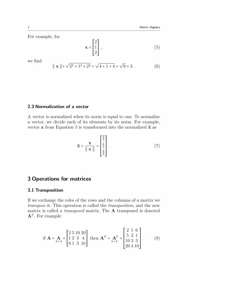
For example, for

x =⎡⎢⎢⎢⎢⎢⎣

212

⎤⎥⎥⎥⎥⎥⎦, (5)

we find∥ x ∥=

√22 + 12 + 22 =

√4 + 1 + 4 =

√9 = 3 . (6)

2.3 Normalization of a vector

A vector is normalized when its norm is equal to one. To normalizea vector, we divide each of its elements by its norm. For example,vector x from Equation 5 is transformed into the normalized x as

x = x

∥ x ∥ =⎡⎢⎢⎢⎢⎢⎢⎢⎣

23

13

23

⎤⎥⎥⎥⎥⎥⎥⎥⎦. (7)

3 Operations for matrices

3.1 Transposition

If we exchange the roles of the rows and the columns of a matrix wetranspose it. This operation is called the transposition, and the newmatrix is called a transposed matrix. The A transposed is denotedAT . For example:

if A = A3×4

=⎡⎢⎢⎢⎢⎢⎣

2 5 10 201 2 3 46 1 3 10

⎤⎥⎥⎥⎥⎥⎦then AT = A

4×3

T =⎡⎢⎢⎢⎢⎢⎢⎢⎣

2 1 65 2 110 3 320 4 10

⎤⎥⎥⎥⎥⎥⎥⎥⎦. (8)

ABDI & WILLIAMS 5

3.2 Addition (sum) of matrices

When two matrices have the same dimensions, we compute theirsum by adding the corresponding elements. For example, with

A =⎡⎢⎢⎢⎢⎢⎣

2 5 10 201 2 3 46 1 3 10

⎤⎥⎥⎥⎥⎥⎦and B =

⎡⎢⎢⎢⎢⎢⎣

3 4 5 62 4 6 81 2 3 5

⎤⎥⎥⎥⎥⎥⎦, (9)

we find

A +B =⎡⎢⎢⎢⎢⎢⎣

2 + 3 5 + 4 10 + 5 20 + 61 + 2 2 + 4 3 + 6 4 + 86 + 1 1 + 2 3 + 3 10 + 5

⎤⎥⎥⎥⎥⎥⎦=⎡⎢⎢⎢⎢⎢⎣

5 9 15 263 6 9 127 3 6 15

⎤⎥⎥⎥⎥⎥⎦. (10)

In general

A +B =

⎡⎢⎢⎢⎢⎢⎢⎢⎢⎣

a1,1 + b1,1 a1,2 + b1,2 ⋯ a1,j + b1,j ⋯ a1,J + b1,Ja2,1 + b2,1 a2,2 + b2,2 ⋯ a2,j + b2,j ⋯ a2,J + b2,J

⋮ ⋮ ⋱ ⋮ ⋱ ⋮ai,1 + bi,1 ai,2 + bi,2 ⋯ ai,j + bi,j ⋯ ai,J + bi,J

⋮ ⋮ ⋱ ⋮ ⋱ ⋮aI,1 + bI,1 aI,2 + bI,2 ⋯ aI,j + bI,j ⋯ aI, J + bI, J

⎤⎥⎥⎥⎥⎥⎥⎥⎥⎦

. (11)

Matrix addition behaves very much like usual addition. Specif-ically, matrix addition is commutative (i.e., A + B = B +A); andassociative [i.e.,A + (B +C) = (A +B) +C].

3.3 Multiplication of a matrix by a scalar

In order to differentiate matrices from the usual numbers, we callthe latter scalar numbers or simply scalars. To multiply a matrixby a scalar, multiply each element of the matrix by this scalar. Forexample:

10 ×B = 10 ×⎡⎢⎢⎢⎢⎢⎣

3 4 5 62 4 6 81 2 3 5

⎤⎥⎥⎥⎥⎥⎦=⎡⎢⎢⎢⎢⎢⎣

30 40 50 6020 40 60 8010 20 30 50

⎤⎥⎥⎥⎥⎥⎦. (12)

6 Matrix Algebra

3.4 Multiplication: Product or products?

There are several ways of generalizing the concept of product tomatrices. We will look at the most frequently used of these matrixproducts. Each of these products will behave like the product be-tween scalars when the matrices have dimensions 1 × 1.

3.5 Hadamard product

When generalizing product to matrices, the first approach is to mul-tiply the corresponding elements of the two matrices that we wantto multiply. This is called the Hadamard product denoted by ⊙. TheHadamard product exists only for matrices with the same dimen-sions. Formally, it is defined as:

A⊙B = [ai,j × bi,j]

=

⎡⎢⎢⎢⎢⎢⎢⎢⎢⎣

a1,1 × b1,1 a1,2 × b1,2 ⋯ a1,j × b1,j ⋯ a1,J × b1,Ja2,1 × b2,1 a2,2 × b2,2 ⋯ a2,j × b2,j ⋯ a2,J × b2,J

⋮ ⋮ ⋱ ⋮ ⋱ ⋮ai,1 × bi,1 ai,2 × bi,2 ⋯ ai,j × bi,j ⋯ ai,J × bi,J

⋮ ⋮ ⋱ ⋮ ⋱ ⋮aI,1 × bI,1 aI,2 × bI,2 ⋯ aI,j × bI,j ⋯ aI, J × bI, J

⎤⎥⎥⎥⎥⎥⎥⎥⎥⎦

. (13)

For example, with

A =⎡⎢⎢⎢⎢⎢⎣

2 5 10 201 2 3 46 1 3 10

⎤⎥⎥⎥⎥⎥⎦and B =

⎡⎢⎢⎢⎢⎢⎣

3 4 5 62 4 6 81 2 3 5

⎤⎥⎥⎥⎥⎥⎦, (14)

we get:

A⊙B =⎡⎢⎢⎢⎢⎢⎣

2 × 3 5 × 4 10 × 5 20 × 61 × 2 2 × 4 3 × 6 4 × 86 × 1 1 × 2 3 × 3 10 × 5

⎤⎥⎥⎥⎥⎥⎦=⎡⎢⎢⎢⎢⎢⎣

6 20 50 1202 8 18 326 2 9 50

⎤⎥⎥⎥⎥⎥⎦. (15)

ABDI & WILLIAMS 7

3.6 Standard (a.k.a.) Cayley product

The Hadamard product is straightforward, but, unfortunately, it isnot the matrix product most often used. This product is called thestandard or Cayley product, or simply the product (i.e., when thename of the product is not specified, this is the standard product). Itsdefinition comes from the original use of matrices to solve equations.Its definition looks surprising at first because it is defined only whenthe number of columns of the first matrix is equal to the numberof rows of the second matrix. When two matrices can be multipliedtogether they are called conformable. This product will have thenumber of rows of the first matrix and the number of columns of thesecond matrix.

So, A with I rows and J columns can be multiplied by B withJ rows and K columns to give C with I rows and K columns. Aconvenient way of checking that two matrices are conformable is towrite the dimensions of the matrices as subscripts. For example:

AI ×J

× BJ ×K

= CI ×K

, (16)

or even:

IA

JB

K= C

I ×K(17)

An element ci,k of the matrix C is computed as:

ci,k =J

∑j=1

ai,j × bj,k . (18)

So, ci,k is the sum of J terms, each term being the product of thecorresponding element of the i-th row of A with the k-th column ofB.

For example, let:

A = [1 2 34 5 6

] and B =⎡⎢⎢⎢⎢⎢⎣

1 23 45 6

⎤⎥⎥⎥⎥⎥⎦. (19)

The product of these matrices is denoted C = A ×B = AB (the ×sign can be omitted when the context is clear). To compute c2,1 we

8 Matrix Algebra

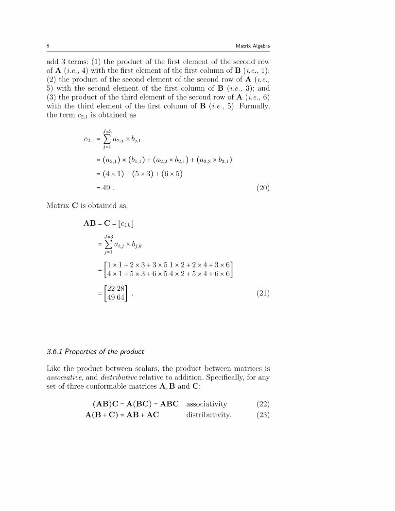
add 3 terms: (1) the product of the first element of the second rowof A (i.e., 4) with the first element of the first column of B (i.e., 1);(2) the product of the second element of the second row of A (i.e.,5) with the second element of the first column of B (i.e., 3); and(3) the product of the third element of the second row of A (i.e., 6)with the third element of the first column of B (i.e., 5). Formally,the term c2,1 is obtained as

c2,1 =J=3∑j=1

a2,j × bj,1

= (a2,1) × (b1,1) + (a2,2 × b2,1) + (a2,3 × b3,1)= (4 × 1) + (5 × 3) + (6 × 5)= 49 . (20)

Matrix C is obtained as:

AB =C = [ci,k]

=J=3∑j=1

ai,j × bj,k

= [1 × 1 + 2 × 3 + 3 × 5 1 × 2 + 2 × 4 + 3 × 64 × 1 + 5 × 3 + 6 × 5 4 × 2 + 5 × 4 + 6 × 6

]

= [22 2849 64

] . (21)

3.6.1 Properties of the product

Like the product between scalars, the product between matrices isassociative, and distributive relative to addition. Specifically, for anyset of three conformable matrices A,B and C:

(AB)C =A(BC) =ABC associativity (22)

A(B +C) =AB +AC distributivity. (23)

ABDI & WILLIAMS 9

The matrix products AB and BA do not always exist, but whenthey do, these products are not, in general, commutative:

AB ≠ BA . (24)

For example, with

A = [ 2 1−2 −1] and B = [ 1 −1

−2 2] (25)

we get:

AB = [ 2 1−2 −1] [

1 −1−2 2

] = [0 00 0

] . (26)

But

BA = [ 1 −1−2 2

] [ 2 1−2 −1] = [ 4 2

−8 −4] . (27)

Incidently, we can combine transposition and product and get thefollowing equation:

(AB)T = BTAT . (28)

3.7 Exotic product: Kronecker

Another product is the Kronecker product also called the direct,tensor, or Zehfuss product. It is denoted ⊗, and is defined for allmatrices. Specifically, with two matrices A = ai,j (with dimensionsI by J) and B (with dimensions K and L), the Kronecker productgives a matrix C (with dimensions (I ×K) by (J ×L)) defined as:

A⊗B =

⎡⎢⎢⎢⎢⎢⎢⎢⎢⎢⎢⎢⎣

a1,1B a1,2B ⋯ a1,jB ⋯ a1,JBa2,1B a2,2B ⋯ a2,jB ⋯ a2,JB⋮ ⋮ ⋱ ⋮ ⋱ ⋮

ai,1B ai,2B ⋯ ai,jB ⋯ ai,JB⋮ ⋮ ⋱ ⋮ ⋱ ⋮

aI,1B aI,2B ⋯ aI,jB ⋯ aI, JB

⎤⎥⎥⎥⎥⎥⎥⎥⎥⎥⎥⎥⎦

. (29)

10 Matrix Algebra

For example, with

A = [1 2 3] and B = [6 78 9

] (30)

we get:

A⊗B = [1 × 6 1 × 7 2 × 6 2 × 7 3 × 6 3 × 71 × 8 1 × 9 2 × 8 2 × 9 3 × 8 3 × 9

] = [6 7 12 14 18 218 9 16 18 24 27

] . (31)

The Kronecker product is used to write design matrices. It isan essential tool for the derivation of expected values and samplingdistributions.

4 Special matrices

Certain special matrices have specific names.

4.1 Square and rectangular matrices

A matrix with the same number of rows and columns is a squarematrix. By contrast, a matrix with different numbers of rows andcolumns, is a rectangular matrix. So:

A =⎡⎢⎢⎢⎢⎢⎣

1 2 34 5 57 8 0

⎤⎥⎥⎥⎥⎥⎦(32)

is a square matrix, but

B =⎡⎢⎢⎢⎢⎢⎣

1 24 57 8

⎤⎥⎥⎥⎥⎥⎦(33)

is a rectangular matrix.

ABDI & WILLIAMS 11

4.2 Symmetric matrix

A square matrix A with ai,j = aj,i is symmetric. So:

A =⎡⎢⎢⎢⎢⎢⎣

10 2 32 20 53 5 30

⎤⎥⎥⎥⎥⎥⎦(34)

is symmetric, but

A =⎡⎢⎢⎢⎢⎢⎣

12 2 34 20 57 8 30

⎤⎥⎥⎥⎥⎥⎦(35)

is not.

Note that for a symmetric matrix:

A =AT . (36)

A common mistake is to assume that the standard product of twosymmetric matrices is commutative. But this is not true as shownby the following example, with:

A =⎡⎢⎢⎢⎢⎢⎣

1 2 32 1 43 4 1

⎤⎥⎥⎥⎥⎥⎦and B =

⎡⎢⎢⎢⎢⎢⎣

1 1 21 1 32 3 1

⎤⎥⎥⎥⎥⎥⎦. (37)

We get

AB =⎡⎢⎢⎢⎢⎢⎣

9 12 1111 15 119 10 19

⎤⎥⎥⎥⎥⎥⎦, but BA =

⎡⎢⎢⎢⎢⎢⎣

9 11 912 15 1011 11 19

⎤⎥⎥⎥⎥⎥⎦. (38)

Note, however, that combining Equations 28 and 36, gives for sym-metric matrices A and B, the following equation:

AB = (BA)T . (39)

12 Matrix Algebra

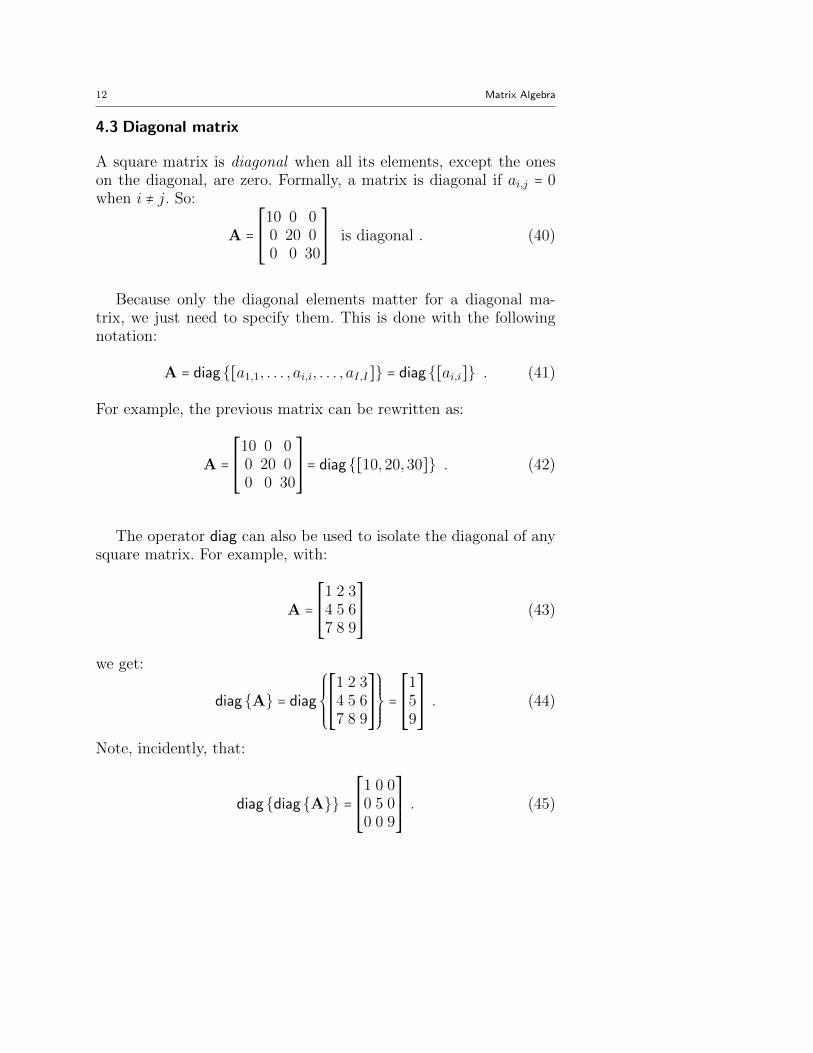
4.3 Diagonal matrix

A square matrix is diagonal when all its elements, except the oneson the diagonal, are zero. Formally, a matrix is diagonal if ai,j = 0when i ≠ j. So:

A =⎡⎢⎢⎢⎢⎢⎣

10 0 00 20 00 0 30

⎤⎥⎥⎥⎥⎥⎦is diagonal . (40)

Because only the diagonal elements matter for a diagonal ma-trix, we just need to specify them. This is done with the followingnotation:

A = diag{[a1,1, . . . , ai,i, . . . , aI,I]} = diag{[ai,i]} . (41)

For example, the previous matrix can be rewritten as:

A =⎡⎢⎢⎢⎢⎢⎣

10 0 00 20 00 0 30

⎤⎥⎥⎥⎥⎥⎦= diag{[10,20,30]} . (42)

The operator diag can also be used to isolate the diagonal of anysquare matrix. For example, with:

A =⎡⎢⎢⎢⎢⎢⎣

1 2 34 5 67 8 9

⎤⎥⎥⎥⎥⎥⎦(43)

we get:

diag{A} = diag

⎧⎪⎪⎪⎨⎪⎪⎪⎩

⎡⎢⎢⎢⎢⎢⎣

1 2 34 5 67 8 9

⎤⎥⎥⎥⎥⎥⎦

⎫⎪⎪⎪⎬⎪⎪⎪⎭=⎡⎢⎢⎢⎢⎢⎣

159

⎤⎥⎥⎥⎥⎥⎦. (44)

Note, incidently, that:

diag{diag{A}} =⎡⎢⎢⎢⎢⎢⎣

1 0 00 5 00 0 9

⎤⎥⎥⎥⎥⎥⎦. (45)

ABDI & WILLIAMS 13

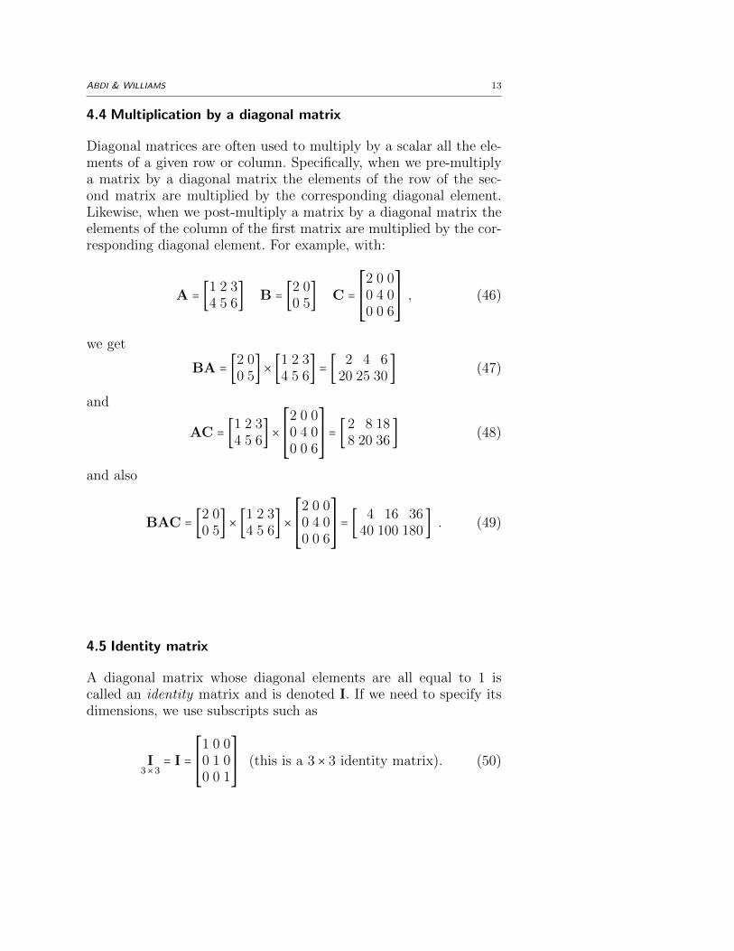
4.4 Multiplication by a diagonal matrix

Diagonal matrices are often used to multiply by a scalar all the ele-ments of a given row or column. Specifically, when we pre-multiplya matrix by a diagonal matrix the elements of the row of the sec-ond matrix are multiplied by the corresponding diagonal element.Likewise, when we post-multiply a matrix by a diagonal matrix theelements of the column of the first matrix are multiplied by the cor-responding diagonal element. For example, with:

A = [1 2 34 5 6

] B = [2 00 5

] C =⎡⎢⎢⎢⎢⎢⎣

2 0 00 4 00 0 6

⎤⎥⎥⎥⎥⎥⎦, (46)

we get

BA = [2 00 5

] × [1 2 34 5 6

] = [ 2 4 620 25 30

] (47)

and

AC = [1 2 34 5 6

] ×⎡⎢⎢⎢⎢⎢⎣

2 0 00 4 00 0 6

⎤⎥⎥⎥⎥⎥⎦= [2 8 18

8 20 36] (48)

and also

BAC = [2 00 5

] × [1 2 34 5 6

] ×⎡⎢⎢⎢⎢⎢⎣

2 0 00 4 00 0 6

⎤⎥⎥⎥⎥⎥⎦= [ 4 16 36

40 100 180] . (49)

4.5 Identity matrix

A diagonal matrix whose diagonal elements are all equal to 1 iscalled an identity matrix and is denoted I. If we need to specify itsdimensions, we use subscripts such as

I3×3

= I =⎡⎢⎢⎢⎢⎢⎣

1 0 00 1 00 0 1

⎤⎥⎥⎥⎥⎥⎦(this is a 3 × 3 identity matrix). (50)

14 Matrix Algebra

The identity matrix is the neutral element for the standard prod-uct. So:

I ×A =A × I =A (51)

for any matrix A conformable with I. For example:

⎡⎢⎢⎢⎢⎢⎣

1 0 00 1 00 0 1

⎤⎥⎥⎥⎥⎥⎦×⎡⎢⎢⎢⎢⎢⎣

1 2 34 5 57 8 0

⎤⎥⎥⎥⎥⎥⎦=⎡⎢⎢⎢⎢⎢⎣

1 2 34 5 57 8 0

⎤⎥⎥⎥⎥⎥⎦×⎡⎢⎢⎢⎢⎢⎣

1 0 00 1 00 0 1

⎤⎥⎥⎥⎥⎥⎦=⎡⎢⎢⎢⎢⎢⎣

1 2 34 5 57 8 0

⎤⎥⎥⎥⎥⎥⎦. (52)

4.6 Matrix full of ones

A matrix whose elements are all equal to 1, is denoted 1 or, when weneed to specify its dimensions, by 1

I ×J. These matrices are neutral

elements for the Hadamard product. So:

A2×3

⊙ 12×3

= [1 2 34 5 6

]⊙ [1 1 11 1 1

] (53)

= [1 × 1 2 × 1 3 × 14 × 1 5 × 1 6 × 1

] = [1 2 34 5 6

] . (54)

The matrices can also be used to compute sums of rows or columns:

[1 2 3] ×⎡⎢⎢⎢⎢⎢⎣

111

⎤⎥⎥⎥⎥⎥⎦= (1 × 1) + (2 × 1) + (3 × 1) = 1 + 2 + 3 = 6 , (55)

or also

[1 1] × [1 2 34 5 6

] = [5 7 9] . (56)

4.7 Matrix full of zeros

A matrix whose elements are all equal to 0, is the null or zero matrix.It is denoted by 0 or, when we need to specify its dimensions, by

ABDI & WILLIAMS 15

0I ×J

. Null matrices are neutral elements for addition

[1 23 4

] + 02×2

= [1 + 0 2 + 03 + 0 4 + 0

] = [1 23 4

] . (57)

They are also null elements for the Hadamard product.

[1 23 4

]⊙ 02×2

= [1 × 0 2 × 03 × 0 4 × 0

] = [0 00 0

] = 02×2

(58)

and for the standard product:

[1 23 4

] × 02×2

= [1 × 0 + 2 × 0 1 × 0 + 2 × 03 × 0 + 4 × 0 3 × 0 + 4 × 0

] = [0 00 0

] = 02×2

. (59)

4.8 Triangular matrix

A matrix is lower triangular when ai,j = 0 for i < j. A matrix is uppertriangular when ai,j = 0 for i > j. For example:

A =⎡⎢⎢⎢⎢⎢⎣

10 0 02 20 03 5 30

⎤⎥⎥⎥⎥⎥⎦is lower triangular, (60)

and

B =⎡⎢⎢⎢⎢⎢⎣

12 2 30 20 50 0 30

⎤⎥⎥⎥⎥⎥⎦is upper triangular. (61)

4.9 Cross-product matrix

A cross-product matrix is obtained by multiplication of a matrixby its transpose. Therefore a cross-product matrix is square andsymmetric. For example, the matrix:

A =⎡⎢⎢⎢⎢⎢⎣

1 12 43 4

⎤⎥⎥⎥⎥⎥⎦(62)

16 Matrix Algebra

pre-multiplied by its transpose

AT = [1 2 31 4 4

] (63)

gives the cross-product matrix:

ATA = [1 × 1 + 2 × 2 + 3 × 3 1 × 1 + 2 × 4 + 3 × 41 × 1 + 4 × 2 + 4 × 3 1 × 1 + 4 × 4 + 4 × 4

]

= [14 2121 33

] . (64)

4.9.1 A particular case of cross-product matrix:Variance/Covariance

A particular case of cross-product matrices are correlation or covari-ance matrices. A variance/covariance matrix is obtained from a datamatrix with three steps: (1) subtract the mean of each column fromeach element of this column (this is “centering”); (2) compute thecross-product matrix from the centered matrix; and (3) divide eachelement of the cross-product matrix by the number of rows of thedata matrix. For example, if we take the I = 3 by J = 2 matrix A:

A =⎡⎢⎢⎢⎢⎢⎣

2 15 108 10

⎤⎥⎥⎥⎥⎥⎦, (65)

we obtain the means of each column as:

m = 1

I× 1

1× I× A

I ×J= 1

3× [1 1 1] ×

⎡⎢⎢⎢⎢⎢⎣

2 15 108 10

⎤⎥⎥⎥⎥⎥⎦= [5 7] . (66)

To center the matrix we subtract the mean of each column from allits elements. This centered matrix gives the deviations from each

ABDI & WILLIAMS 17

element to the mean of its column. Centering is performed as:

D =A − 1J ×1

×m =⎡⎢⎢⎢⎢⎢⎣

2 15 108 10

⎤⎥⎥⎥⎥⎥⎦−⎡⎢⎢⎢⎢⎢⎣

111

⎤⎥⎥⎥⎥⎥⎦× [5 7] (67)

=⎡⎢⎢⎢⎢⎢⎣

2 15 108 10

⎤⎥⎥⎥⎥⎥⎦−⎡⎢⎢⎢⎢⎢⎣

5 75 75 7

⎤⎥⎥⎥⎥⎥⎦=⎡⎢⎢⎢⎢⎢⎣

−3 −60 33 3

⎤⎥⎥⎥⎥⎥⎦. (68)

We note S the variance/covariance matrix derived from A, it iscomputed as:

S = 1

IDTD = 1

3[−3 0 3−6 3 3] ×

⎡⎢⎢⎢⎢⎢⎣

−3 −60 33 3

⎤⎥⎥⎥⎥⎥⎦= 1

3× [18 27

27 54] = [6 9

9 18] . (69)

(Variances are on the diagonal, covariances are off-diagonal.)

5 The inverse of a square matrix

An operation similar to division exists, but only for (some) squarematrices. This operation uses the notion of inverse operation anddefines the inverse of a matrix. The inverse is defined by analogywith the scalar number case for which division actually correspondsto multiplication by the inverse, namely:

a

b= a × b−1 with b × b−1 = 1 . (70)

The inverse of a square matrix A is denoted A−1. It has thefollowing property:

A ×A−1 =A−1 ×A = I . (71)

18 Matrix Algebra

The definition of the inverse of a matrix is simple. but its computa-tion, is complicated and is best left to computers.

For example, for:

A =⎡⎢⎢⎢⎢⎢⎣

1 2 10 1 00 0 1

⎤⎥⎥⎥⎥⎥⎦, (72)

the inverse is:

A−1 =⎡⎢⎢⎢⎢⎢⎣

1 −2 −10 1 00 0 1

⎤⎥⎥⎥⎥⎥⎦. (73)

All square matrices do not necessarily have an inverse. The inverseof a matrix does not exist if the rows (and the columns) of this matrixare linearly dependent. For example,

A =⎡⎢⎢⎢⎢⎢⎣

3 4 21 0 22 1 3

⎤⎥⎥⎥⎥⎥⎦, (74)

does not have an inverse since the second column is a linear combi-nation of the two other columns:

⎡⎢⎢⎢⎢⎢⎣

401

⎤⎥⎥⎥⎥⎥⎦= 2 ×

⎡⎢⎢⎢⎢⎢⎣

312

⎤⎥⎥⎥⎥⎥⎦−⎡⎢⎢⎢⎢⎢⎣

223

⎤⎥⎥⎥⎥⎥⎦=⎡⎢⎢⎢⎢⎢⎣

624

⎤⎥⎥⎥⎥⎥⎦−⎡⎢⎢⎢⎢⎢⎣

223

⎤⎥⎥⎥⎥⎥⎦. (75)

A matrix without an inverse is singular. WhenA−1 exists it is unique.

Inverse matrices are used for solving linear equations, and leastsquare problems in multiple regression analysis or analysis of vari-ance.

ABDI & WILLIAMS 19

5.1 Inverse of a diagonal matrix

The inverse of a diagonal matrix is easy to compute: The inverse of

A = diag{ai,i} (76)

is the diagonal matrix

A−1 = diag{a−1i,i} = diag{1/ai,i} (77)

For example, ⎡⎢⎢⎢⎢⎢⎣

1 0 00 .5 00 0 4

⎤⎥⎥⎥⎥⎥⎦and

⎡⎢⎢⎢⎢⎢⎣

1 0 00 2 00 0 .25

⎤⎥⎥⎥⎥⎥⎦, (78)

are the inverse of each other.

6 The Big tool: eigendecomposition

So far, matrix operations are very similar to operations with num-bers. The next notion is specific to matrices. This is the idea ofdecomposing a matrix into simpler matrices. A lot of the power ofmatrices follows from this. A first decomposition is called the eigen-decomposition and it applies only to square matrices, the generaliza-tion of the eigendecomposition to rectangular matrices is called thesingular value decomposition.

Eigenvectors and eigenvalues are numbers and vectors associatedwith square matrices, together they constitute the eigendecompo-sition. Even though the eigendecomposition does not exist for allsquare matrices, it has a particularly simple expression for a classof matrices often used in multivariate analysis such as correlation,covariance, or cross-product matrices. The eigendecomposition ofthese matrices is important in statistics because it is used to findthe maximum (or minimum) of functions involving these matrices.For example, principal component analysis is obtained from the ei-gendecomposition of a covariance or correlation matrix and gives theleast square estimate of the original data matrix.

20 Matrix Algebra

6.1 Notations and definition

An eigenvector of matrix A is a vector u that satisfies the followingequation:

Au = λu , (79)

where λ is a scalar called the eigenvalue associated to the eigenvector.When rewritten, Equation 79 becomes:

(A − λI)u = 0 . (80)

Therefore u is eigenvector of A if the multiplication of u by Achanges the length of u but not its orientation. For example,

A = [2 32 1

] (81)

has for eigenvectors:

u1 = [32] with eigenvalue λ1 = 4 (82)

and

u2 = [−11] with eigenvalue λ2 = −1 (83)

When u1 and u2 are multiplied by A, only their length changes.That is,

Au1 = λ1u1 = [2 32 1

] [32] = [12

8] = 4 [3

2] (84)

and

Au2 = λ2u2 = [2 32 1

] [−11] = [ 1

−1] = −1 [−11] . (85)

This is illustrated in Figure 1.

For convenience, eigenvectors are generally normalized such that:

uTu = 1 . (86)

ABDI & WILLIAMS 21

3

2

12

8

u1

1Au

-1

11

-1

u

Au

a b

2

2

Figure 1: Two eigenvectors of a matrix.

For the previous example, normalizing the eigenvectors gives:

u1 = [.8321.5547

] and u2 [−.7071.7071] . (87)

We can check that:

[2 32 1

] [.8321.5547

] = [3.32842.2188

] = 4 [.8321.5547

] (88)

and

[2 32 1

] [−.7071.7071

] = [ .7071−.7071] = −1 [

−.7071.7071

] . (89)

6.2 Eigenvector and eigenvalue matrices

Traditionally, we store the eigenvectors of A as the columns a matrixdenoted U. Eigenvalues are stored in a diagonal matrix (denoted Λ).Therefore, Equation 79 becomes:

AU =UΛ . (90)

22 Matrix Algebra

For example, with A (from Equation 81), we have

[2 32 1

] × [3 −12 1

] = [3 −12 1

] × [4 00 −1] (91)

6.3 Reconstitution of a matrix

The eigen-decomposition can also be use to build back a matrix fromit eigenvectors and eigenvalues. This is shown by rewriting Equation90 as

A =UΛU−1 . (92)

For example, because

U−1 = [ .2 .2−.4 .6] ,

we obtain:

A =UΛU−1

= [3 −12 1

] [4 00 −1] [

.2 .2−.4 .6]

= [2 32 1

] . (93)

6.4 Digression:An infinity of eigenvectors for one eigenvalue

It is only through a slight abuse of language that we talk about theeigenvector associated with one eigenvalue. Any scalar multiple ofan eigenvector is an eigenvector, so for each eigenvalue there is aninfinite number of eigenvectors all proportional to each other. Forexample,

[ 1−1] (94)

ABDI & WILLIAMS 23

is an eigenvector of A:

[2 32 1

] . (95)

Therefore:

2 × [ 1−1] = [ 2

−2] (96)

is also an eigenvector of A:

[2 32 1

] [ 2−2] = [−2

2] = −1 × 2 [ 1

−1] . (97)

6.5 Positive (semi-)definite matrices

Some matrices, such as [0 10 0

], do not have eigenvalues. Fortunately,

the matrices used often in statistics belong to a category called pos-itive semi-definite. The eigendecomposition of these matrices alwaysexists and has a particularly convenient form. A matrix is positivesemi-definite when it can be obtained as the product of a matrix byits transpose. This implies that a positive semi-definite matrix is al-ways symmetric. So, formally, the matrix A is positive semi-definiteif it can be obtained as:

A =XXT (98)

for a certain matrix X. Positive semi-definite matrices include cor-relation, covariance, and cross-product matrices.

The eigenvalues of a positive semi-definite matrix are always pos-itive or null. Its eigenvectors are composed of real values and arepairwise orthogonal when their eigenvalues are different. This im-plies the following equality:

U−1 =UT . (99)

We can, therefore, express the positive semi-definite matrix A as:

A =UΛUT (100)

where UTU = I are the normalized eigenvectors.

24 Matrix Algebra

For example,

A = [3 11 3

] (101)

can be decomposed as:

A =UΛUT

=⎡⎢⎢⎢⎢⎢⎣

√12

√12√

12 −

√12

⎤⎥⎥⎥⎥⎥⎦[4 00 2

]⎡⎢⎢⎢⎢⎢⎣

√12

√12√

12 −

√12

⎤⎥⎥⎥⎥⎥⎦

= [3 11 3

] , (102)

with ⎡⎢⎢⎢⎢⎢⎣

√12

√12√

12 −

√12

⎤⎥⎥⎥⎥⎥⎦

⎡⎢⎢⎢⎢⎢⎣

√12

√12√

12 −

√12

⎤⎥⎥⎥⎥⎥⎦= [1 0

0 1] . (103)

6.5.1 Diagonalization

When a matrix is positive semi-definite we can rewrite Equation 100as

A =UΛUT⇐⇒ Λ =UTAU . (104)

This shows that we can transform A into a diagonal matrix. There-fore the eigen-decomposition of a positive semi-definite matrix isoften called its diagonalization.

6.5.2 Another definition for positive semi-definite matrices

A matrix A is positive semi-definite if for any non-zero vector x wehave:

xTAx ≥ 0 ∀x . (105)

When all the eigenvalues of a matrix are positive, the matrix ispositive definite. In that case, Equation 105 becomes:

xTAx > 0 ∀x . (106)

ABDI & WILLIAMS 25

6.6 Trace, Determinant, etc.

The eigenvalues of a matrix are closely related to three importantnumbers associated to a square matrix the: trace, determinant andrank.

6.6.1 Trace

The trace of A, denoted trace{A}, is the sum of its diagonal ele-ments. For example, with:

A =⎡⎢⎢⎢⎢⎢⎣

1 2 34 5 67 8 9

⎤⎥⎥⎥⎥⎥⎦(107)

we obtain:trace{A} = 1 + 5 + 9 = 15 . (108)

The trace of a matrix is also equal to the sum of its eigenvalues:

trace{A} =∑`

λ` = trace{Λ} (109)

with Λ being the matrix of the eigenvalues of A. For the previousexample, we have:

Λ = diag{16.1168,−1.1168,0} . (110)

We can verify that:

trace{A} =∑`

λ` = 16.1168 + (−1.1168) = 15 (111)

6.6.2 Determinant

The determinant is important for finding the solution of systems oflinear equations (i.e., the determinant determines the existence of asolution). The determinant of a matrix is equal to the product of its

26 Matrix Algebra

eigenvalues. If det{A} is the determinant of A:

det{A} =∏`

λ` with λ` being the `-th eigenvalue of A . (112)

For example, the determinant of A from Equation 107 is equal to:

det{A} = 16.1168 × −1.1168 × 0 = 0 . (113)

6.6.3 Rank

Finally, the rank of a matrix is the number of non-zero eigenvaluesof the matrix. For our example:

rank{A} = 2 . (114)

The rank of a matrix gives the dimensionality of the Euclidean spacewhich can be used to represent this matrix. Matrices whose rank isequal to their dimensions are full rank and they are invertible. Whenthe rank of a matrix is smaller than its dimensions, the matrix is notinvertible and is called rank-deficient, singular, or multicolinear. Forexample, matrix A from Equation 107, is a 3 × 3 square matrix, itsrank is equal to 2, and therefore it is rank-deficient and does nothave an inverse.

6.7 Statistical properties of the eigen-decomposition

The eigen-decomposition is essential in optimization. For example,principal component analysis (pca) is a technique used to analyze aI ×J matrix X where the rows are observations and the columns arevariables. Pca finds orthogonal row factor scores which “explain”as much of the variance of X as possible. They are obtained as

F =XQ , (115)

where F is the matrix of factor scores and Q is the matrix of loadingsof the variables. These loadings give the coefficients of the linearcombination used to compute the factor scores from the variables.

ABDI & WILLIAMS 27

In addition to Equation 115 we impose the constraints that

FTF =QTXTXQ (116)

is a diagonal matrix (i.e., F is an orthogonal matrix) and that

QTQ = I (117)

(i.e., Q is an orthonormal matrix). The solution is obtained by usingLagrangian multipliers where the constraint from Equation 117 isexpressed as the multiplication with a diagonal matrix of Lagrangianmultipliers denoted Λ in order to give the following expression

Λ (QTQ − I) (118)

This amounts to defining the following equation

L = trace{FTF −Λ (QTQ − I)} = trace{QTXTXQ −Λ (QTQ − I)} .(119)

The values of Q which give the maximum values of L, are found byfirst computing the derivative of L relative to Q:

∂L∂Q

= 2XTXQ − 2ΛQ, (120)

and setting this derivative to zero:

XTXQ −ΛQ = 0⇐⇒XTXQ = ΛQ . (121)

Because Λ is diagonal, this is an eigendecomposition problem, andΛ is the matrix of eigenvalues of the positive semi-definite matrixXTX ordered from the largest to the smallest and Q is the matrixof eigenvectors of XTX. Finally, the factor matrix is

F =XQ . (122)

The variance of the factors scores is equal to the eigenvalues:

FTF =QTXTXQ = Λ . (123)

28 Matrix Algebra

Because the sum of the eigenvalues is equal to the trace of XTX, thefirst factor scores “extract” as much of the variances of the originaldata as possible, and the second factor scores extract as much ofthe variance left unexplained by the first factor, and so on for the

remaining factors. The diagonal elements of the matrix Λ12 which are

the standard deviations of the factor scores are called the singularvalues of X.

7 A tool for rectangular matrices:

The singular value decomposition

The singular value decomposition (svd) generalizes the eigendecom-position to rectangular matrices. The eigendecomposition, decom-poses a matrix into two simple matrices, and the svd decomposes arectangular matrix into three simple matrices: Two orthogonal ma-trices and one diagonal matrix. The svd uses the eigendecompositionof a positive semi-definite matrix to derive a similar decompositionfor rectangular matrices.

7.1 Definitions and notations

The svd decomposes matrix A as:

A = P∆QT . (124)

where P is the (normalized) eigenvectors of the matrix AAT (i.e.,

PTP = I). The columns of P are called the left singular vectorsof A. Q is the (normalized) eigenvectors of the matrix ATA (i.e.,QTQ = I). The columns of Q are called the right singular vectors of

A. ∆ is the diagonal matrix of the singular values, ∆ = Λ12 with Λ

being the diagonal matrix of the eigenvalues of AAT and ATA.

The svd is derived from the eigendecomposition of a positivesemi-definite matrix. This is shown by considering the eigendecom-position of the two positive semi-definite matrices obtained from A:

ABDI & WILLIAMS 29

namely AAT and ATA. If we express these matrices in terms of thesvd of A, we find:

AAT = P∆QTQ∆PT = P∆2PT = PΛPT , (125)

andATA =Q∆PTP∆QT =Q∆2QT =QΛQT . (126)

This shows that∆ is the square root of Λ, that P are eigenvectorsof AAT, and that Q are eigenvectors of ATA.

For example, the matrix:

A =⎡⎢⎢⎢⎢⎢⎣

1.1547 −1.1547−1.0774 0.0774−0.0774 1.0774

⎤⎥⎥⎥⎥⎥⎦(127)

can be expressed as:

A = P∆QT

=⎡⎢⎢⎢⎢⎢⎣

0.8165 0−0.4082 −0.7071−0.4082 0.7071

⎤⎥⎥⎥⎥⎥⎦[2 00 1

] [ 0.7071 0.7071−0.7071 0.7071

]

=⎡⎢⎢⎢⎢⎢⎣

1.1547 −1.1547−1.0774 0.0774−0.0774 1.0774

⎤⎥⎥⎥⎥⎥⎦. (128)

We can check that:

AAT =⎡⎢⎢⎢⎢⎢⎣

0.8165 0−0.4082 −0.7071−0.4082 0.7071

⎤⎥⎥⎥⎥⎥⎦[2

2 00 12

] [ 0.8165 −0.4082 −0.40820 −0.7071 0.7071

]

30 Matrix Algebra

=⎡⎢⎢⎢⎢⎢⎣

2.6667 −1.3333 −1.3333−1.3333 1.1667 0.1667−1.3333 0.1667 1.1667

⎤⎥⎥⎥⎥⎥⎦(129)

and that:

ATA = [ 0.7071 0.7071−0.7071 0.7071

] [22 00 12

] [ 0.7071 −0.70710.7071 0.7071

]

= [ 2.5 −1.5−1.5 2.5

] . (130)

7.2 Generalized or pseudo-inverse

The inverse of a matrix is defined only for full rank square matri-ces. The generalization of the inverse for other matrices is calledgeneralized inverse, pseudo-inverse or Moore-Penrose inverse and isdenoted by X+. The pseudo-inverse of A is the unique matrix thatsatisfies the following four constraints:

AA+A =A (i)A+AA+ =A+ (ii)(AA+)T =AA+ (symmetry 1) (iii)(A+A)T =A+A (symmetry 2) (iv) . (131)

For example, with

A =⎡⎢⎢⎢⎢⎢⎣

1 −1−1 11 1

⎤⎥⎥⎥⎥⎥⎦(132)

we find that the pseudo-inverse is equal to

A+ = [ .25 −.25 .5−.25 .25 .5

] . (133)

ABDI & WILLIAMS 31

This example shows that the product of a matrix and its pseudo-inverse does not always gives the identity matrix:

AA+ =⎡⎢⎢⎢⎢⎢⎣

1 −1−1 11 1

⎤⎥⎥⎥⎥⎥⎦[ .25 −.25 .5−.25 .25 .5

] = [0.3750 0.12500.1250 0.3750

] . (134)

7.3 Pseudo-inverse and singular value decomposition

The svd is the building block for the Moore-Penrose pseudo-inverse.Because any matrix A with svd equal to P∆QT has for pseudo-inverse:

A+ =Q∆−1PT . (135)

For the preceding example we obtain:

A+ = [ 0.7071 0.7071−0.7071 0.7071

] [2−1 00 1−1] [

0.8165 −0.4082 −0.40820 −0.7071 0.7071

]

= [ 0.2887 −0.6443 0.3557−0.2887 −0.3557 0.6443

] . (136)

Pseudo-inverse matrices are used to solve multiple regression andanalysis of variance problems.

Related entries

Analysis of variance and covariance, canonical correlation, corre-spondence analysis, confirmatory factor analysis, discriminant analy-sis, general linear, latent variable, Mauchly test, multiple regression,principal component analysis, sphericity, structural equation mod-elling

32 Matrix Algebra

Further readings

1. Abdi, H. (2007a). Eigendecomposition: eigenvalues and eigen-vecteurs. In N.J. Salkind (Ed.): Encyclopedia of Measurementand Statistics. Thousand Oaks (CA): Sage. pp. 304–308.

2. Abdi, H. (2007b). Singular Value Decomposition (SVD) andGeneralized Singular Value Decomposition (GSVD). In N.J.Salkind (Ed.): Encyclopedia of Measurement and Statistics.Thousand Oaks (CA): Sage. pp. 907–912.

3. Basilevsky, A. (1983). Applied Matrix Algebra in the StatisticalSciences. New York: North-Holland.

4. Graybill, F.A. (1969). Matrices with Applications in Statistics.New York: Wadworth.

5. Healy, M.J.R. (1986). Matrices for Statistics. Oxford: OxfordUniversity Press.

6. Searle, S.R. (1982). Matrices Algebra Useful for Statistics. NewYork: Wiley.