1 increase malaysia palm oil production efficiency yik nam - bora
TRANSCRIPT

1
Increase Malaysia Palm Oil Production efficiency
Yik Nam,Lee
Submitted in Partial Fulfilment of the Requirements for the Degree of
Master of Philosophy in System Dynamics
System Dynamics Group,
Faculty of Social Sciences
University of Bergen
November, 2011
2
LIST OF TABLE AND FIGURE
ABSTRACT
Malaysia is the second largest palm oil producer in the world. It has been suffering from
low production efficiency for over 20 years. This paper tries to identify factors cause
the low production efficiency by using system dynamics method. A model has been
built to explain and further study slow improvement of production. The model also
serves as a tool for explaining the problematic behaviours and understanding the
feedbacks influence both oil palm area expansion and foreign labour workforce.
Production efficiency is sensitive to high yield area fresh fruit branch yield rate, mature
time and oil extraction rate. Production efficiency has weak relationship to labour.
Policies to improve production efficiency has been suggested to improve the production
efficiency within ten years.
Key words: palm oil, production efficiency, system dynamics, workforce.

3
ACKNOWLEDGEMENTS
I have been very please to have David Wheat as my supervisor. His teaching in system
dynamics has inspired me for understanding the complex system can be comprehend
with different methods.
I also want to thank Malaysia government, which provide detail information to
everyone who can access to the internet. This information is very useful to me and I
appreciate with it.
Finally, thanks to researchers from internet contribute their life on writing papers which
really help me a lot on sharing knowledge with me.
4
INTRODUCTION
Malaysia’s palm oil industry is the fourth largest contributor to the national
economy [1].
The oil palm industry in Malaysia is export oriented industry. It is heavily
depends on the world market. Most of the palm oil production has exported to foreign
countries, only 10% of which is consumed by locals. As the world’s palm oil demand is
growing quickly, it is expected, both Indonesia and Malaysia will keep dominating the
oil palm industry. The oil palm industry in Malaysia is very competitive and become
one of the major economic sectors contributing to the total revenue of the country [2] .
In year 2009, there was a total of 22.40 million tons of oil palm products
including palm oil, palm kernel oil, palm kernel cake, oleo-chemicals and finished
products, equivalent to RM 49.59 billion of export revenue. [2] .
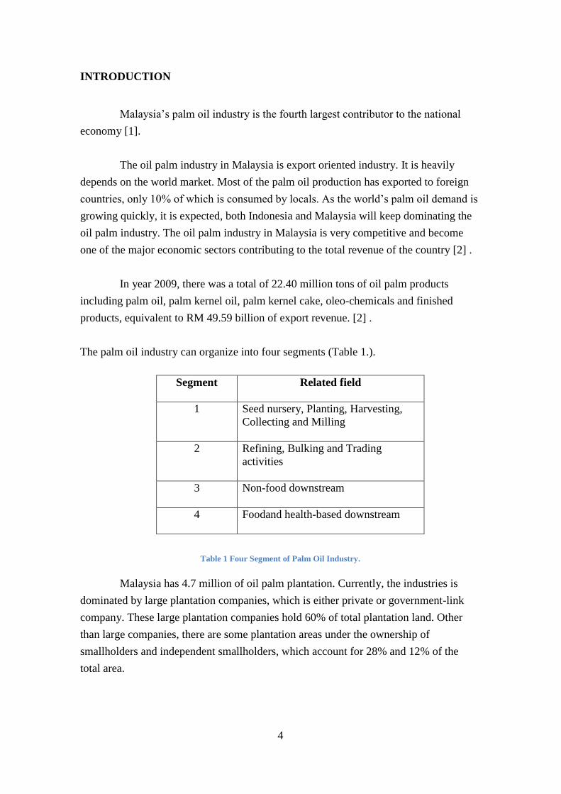
The palm oil industry can organize into four segments (Table 1.).
Segment
Related field
1 Seed nursery, Planting, Harvesting,
Collecting and Milling
2 Refining, Bulking and Trading
activities
3 Non-food downstream
4 Foodand health-based downstream
Table 1 Four Segment of Palm Oil Industry.
Malaysia has 4.7 million of oil palm plantation. Currently, the industries is
dominated by large plantation companies, which is either private or government-link
company. These large plantation companies hold 60% of total plantation land. Other
than large companies, there are some plantation areas under the ownership of
smallholders and independent smallholders, which account for 28% and 12% of the
total area.
5
Palm oil industry has 2 core advantages over other substitutes:
Strong demand
The demand for palm oil has increased sharply. It is driven by increasing
global population. Average growth rate of global demand for oil and fats is 7% over the
past ten years, over the same period palm oil has grown at 10% rate.
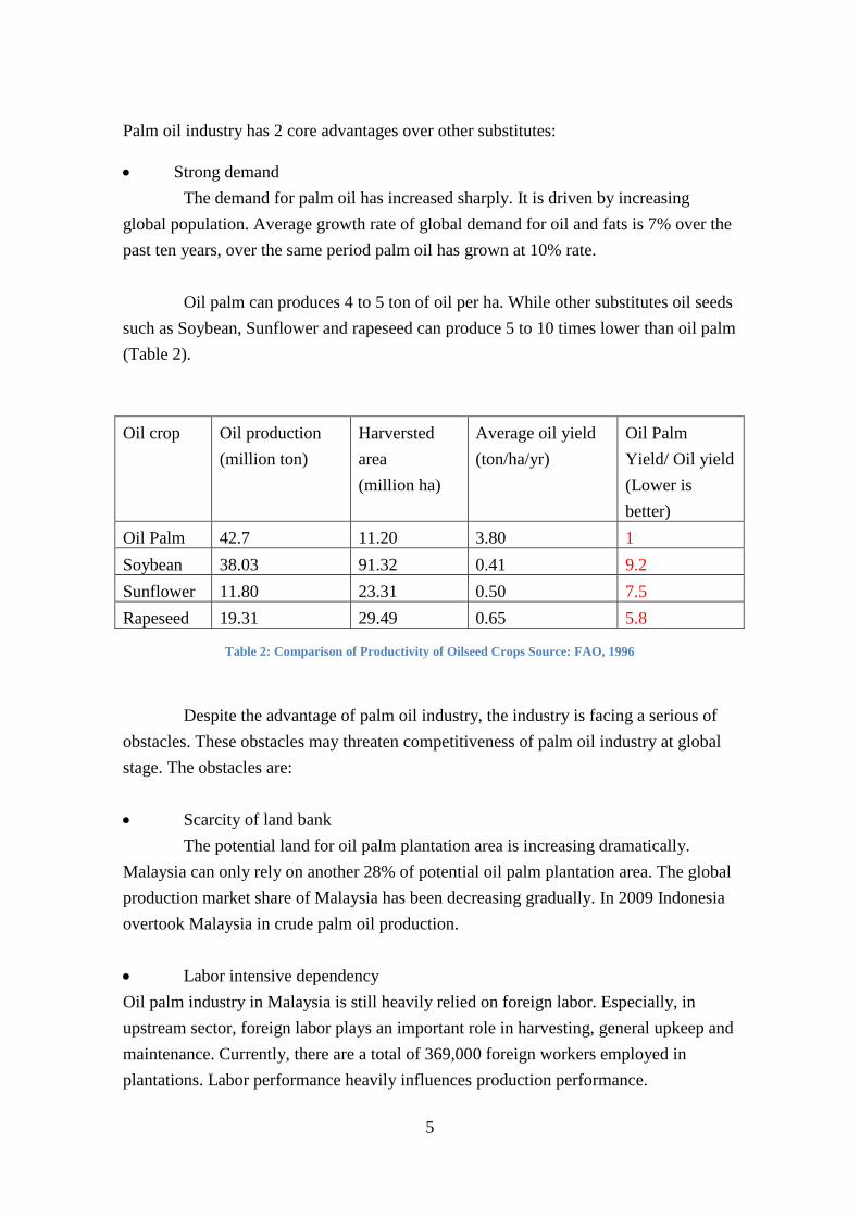
Oil palm can produces 4 to 5 ton of oil per ha. While other substitutes oil seeds
such as Soybean, Sunflower and rapeseed can produce 5 to 10 times lower than oil palm
(Table 2).
Oil crop Oil production
(million ton)
Harversted
area
(million ha)
Average oil yield
(ton/ha/yr)
Oil Palm
Yield/ Oil yield
(Lower is
better)
Oil Palm 42.7 11.20 3.80 1
Soybean 38.03 91.32 0.41 9.2
Sunflower 11.80 23.31 0.50 7.5
Rapeseed 19.31 29.49 0.65 5.8
Table 2: Comparison of Productivity of Oilseed Crops Source: FAO, 1996
Despite the advantage of palm oil industry, the industry is facing a serious of
obstacles. These obstacles may threaten competitiveness of palm oil industry at global
stage. The obstacles are:
Scarcity of land bank
The potential land for oil palm plantation area is increasing dramatically.
Malaysia can only rely on another 28% of potential oil palm plantation area. The global
production market share of Malaysia has been decreasing gradually. In 2009 Indonesia
overtook Malaysia in crude palm oil production.
Labor intensive dependency
Oil palm industry in Malaysia is still heavily relied on foreign labor. Especially, in
upstream sector, foreign labor plays an important role in harvesting, general upkeep and
maintenance. Currently, there are a total of 369,000 foreign workers employed in
plantations. Labor performance heavily influences production performance.
6
Environment concerns
Anti-palm oil campaigns have become stronger. According to the research, oil
palm plantation development has been descripted as “a poor substitute for natural
forests” (Emily Fitzherbert, 2008). The claims from Anti-palm oil campaigns have
generated a negative impact on perception of palm oil. The purpose of anti-palm oil
campaigns is to slow down the acceleration of deforestation because of oil palm
plantation expansion.
In September 21, 2010, Malaysia government has launched a programme,
called Economic Transformation Programme. One of the programme related to oil palm
development suggest that dependency of foreign worker will be reduced by 15% to 20%
as a result of major gains in worker productivity, which is equivalent to reducing of
110,000 foreign workers.
The programme also target a 25% increase in national average FFB yield.
Currently the average FFB yield is 21 ton per ha per year. By 2020, average FFB yield
should achieve 26.2 ton per ha per year.
Oil extraction rate has not been improved over the past 10 year. Date to 2009,
it averaged 20.5% in 2009. Economic Transformation Programme target a 23% oil
extraction rate by 2020.
The focus for this paper is to model the slow improvement on production
efficiency and test the policy options from Economic Transformation Programme. Then
Suggesting a better policy which can aid achieve Economic Transformation
Programme’s to achieve its goal.

7
LITERATURE REVIEW
Malaysia oil palm industry faces many challenges for years. One of those
challenges is low palm oil yield rate. Palm oil yield rate is caused by low palm oil
production rate and high land usage. Low yield decrease production rate, but increases
land usage. Low yield rate decrease the average oil extraction rate. Increasing land
usage raises number of worker and increase production cost. Mini tractor grabber is
introduce to lower the production cost.
As a second, largest palm oil producer in the world, Malaysia is benefit from
palm oil. Claire Carter, Willa Finley, James Fry,David Jackson and Lynn Willis
(2007)[3], analyzed global crude palm oil supply and output, Claire Carter et al.
compared the palm oil production, yield rate with other vegetable oil as well as oil
price with other global major vegetable oils, they found that palm oil has advantages
over other vegetable in production rate, sell price, production cost and yield rate. Yusof
Basiron (2007)[4] also agreed with Claire et al. He found that oil palm is highly
productive crop, which produces tenfold higher yield of oil than other. In other words,
oil palm uses comparatively less land than other edible oil industry, and hence palm oil
has no strong competitor, in term of price and production rate.
As the nature of oil palm, Claire et al. (2007) gave their conclusion on palm oil
development that palm oil industry growth as long as there is willingness to plant more
oil palm in environment sensitive areas and relatively lower price on demanding palm
oil. Thus, palm oil production can increase, if environment and labor concern can be
overcome. Abbai Belai et al.(2010) state that Malaysia currently has already turned 4.6
million hectare of agriculture land into oil palm area, which is account for 70% of total
agricultural land[5]. Thus, land scarcity pressure is becoming higher.
How will oil palm expansion affect biodiversity? There are little research on
how oil palm expansion affects biodiversity, especially in Malaysia. But Emily B.
Fitzherbert, Matthew J. Struebig, Alexandra Morel, Finn Danielsen, Carsten A. Bru¨ hl,
Paul F. Donald and Ben Phalan (2008)[6] compare the statistical data and the diversity
of oil palm, they claimed that increasing the productivity of palm oil production from
harvesting gain would only generate a conservation gain if it was linked to the
protection of natural habitats. With high yield per unit area could reduce the area of land
needed. In summary, Emily B et al. state that “oil palm is a particularly poor substitute
for either primary or degraded forests, and whereas any conversion of natural forest is

8
inevitably damaging to biodiversity, oil palm plantations support even fewer forest
species than do most other agricultural options” . Therefore, oil palm is not an ideal
replacement for natural forest.
If oil palm expansion is not a good alternative way to respond to the inevitable
increasing demand of oil palm, increasing production in existing plantation could be
one of the solution. Khoo Khee Ming and D Chandramohan (2002) [7] predicted the
gap of between low and high yield (yield rate) will come down in the future as the
lower yield palm are replanted by comparing best practice and national average yield
rate. But Khoo et al.(2002) did not explain how low yield palm will be replanted. But It
seems that replanting oil palm can increase the yield rate.
However, Claire et al. (2007) did raise two concerns on palm oil harvesting
process. First palm oil industry is still a labor-intensive system. Second, It is practically
difficult to mechanize. These two concerns were becoming more burdensome as labor
shortage pressure push up wage rates. With high wage rate, it might increase the palm
oil production cost and decrease palm oil competitiveness. These two behaviors have
been addressed by Abbai Belai et al. (2008).
A labor-intensive oil palm system could be vulnerable to labor workforce.
Khoo et al. referenced a survey from Malaysia Agricultural and stated that worker
dependency in west and east Malaysia were 40% and 37% respectively. He also state
that Malaysia policy were confusing. The frequent abrupt changes in policy caused the
shortage of workers. At the same time, recruitment and employment costs have been
pushed ahead, which adding the production cost. Khoo et al’s view, indeed, is similar to
Claire et al, which labor shortage increased production cost.
The Malaysian Palm Oil Cluster Final Report[5] which written by Abbai Belai,
Daniel Boakye, John Vrakas, Hashim Wasswa(2011) shows that the recent growth of
palm oil was result in increasing in edible oil globally. Malaysia has managed to
increase its productivity through innovation. Abbai Belai et al. compiled a table and
point out that Labor cost in Malaysia was higher than Indonesia which is the largest
palm oil producer. Malaysia labor cost was 4.5 dollar per hours, while Indonesia was
only 0.6. Thus, labor cost could be one of the major problems for oil palm.
To reduce production cost, mechanization in oil palm plantation is has been
considered. Abbai Belai et al. (2008) found that in palm oil harvesting 75% of FFB
collection is rely on manual labor and 25% is done mostly through mini tractor grabber.

9
The mini tractor grabber has 5 year life time, which is as long as foreign labor tenures
ends time.
Jalani, B S et al.(2002)[8] concluded that mechanization and automation are to
be adopted in all sectors from oil palm planting to processing because of current low
productivity. The increased productivity and yield would help supply the growing
demand of oil. Jalani et al. examined a few factors causing low productivity, such as
marginal areas, inadequate agronomic inputs, ineffective and inadequate management,
shortage of skilled labor and low replanting Rate. These factors, indeed can group into
3 categories, which are land, labor workforce and management. Jalani et al. also raised
the similar issues as other scholars. One different statement was low productivity could
lower down average oil extraction rate1.
How yield per unit area per year affects by production rate and land usage for
oil palm and whether yield rate have strong effect on labour number. The thesis will
answer clarified the issue and answer the doubt.
1 We should make it clear that average oil extraction rate is different from oil extraction rate. Average
oil extraction rate is an average of yield fresh fruit towards oil production in general. However, oil
extraction rate is capability of a machine to extract oil palm. Therefore, oil extraction rate is
machine dependence

10
Contents
LIST OF TABLE AND FIGURE 2
ABSTRACT 2
ACKNOWLEDGEMENTS 3
LITERATURE REVIEW 7
THE DYNAMIC PROBLEM 12
HYPOTHESIS 13
Hypothesis overview 13
Causal loop diagram: Capacity Section 14
MODEL STRUCTURE 20
The Model Boundary 20
Time Horizon 21
The Stock and Flow Structures 21
The capacity oil palm section 22 The production section 24
The workforce section 25
ANALYSIS 27
Equilibrium shock test 27
Capacity Section 30
Cutting C1 Loop 30 Cutting C2 Loop 31
Cutting R2 Loop 31 Cutting R3 Loop 32
Cutting R4 Loop 32 Workforce Section 33
Cutting C3 Loop 33 Cutting C4 Loop 34
Sensitivity analysis 36
Mature time 36
FFB yield per high yield area per year 36 FFB yield per deteriorated area per year 37 Oil extraction rate 38
Simulation settings 38
Recreation of reference mode 39
Historical production rate and simulation production rate 41
Historical total oil palm area and simulation oil palm area 42
Reference mode: Sensitivity test 44
Mature time 44 FFB yield per high yield area per year 45 Oil extraction rate 45

11
POLICY 46
ETP 2020 goal: Error! Bookmark not defined.
Policy Option 1 46
Analysis of Policy option 1 46
Policy Option 1 testing 47
Policy Option 2 50
Policy Option 2 testing 50
Scenario testing for policies option 1 and 2 51
CONCLUSION 54
APPENDIX 55
Equations 55
REFERENCES 67
12
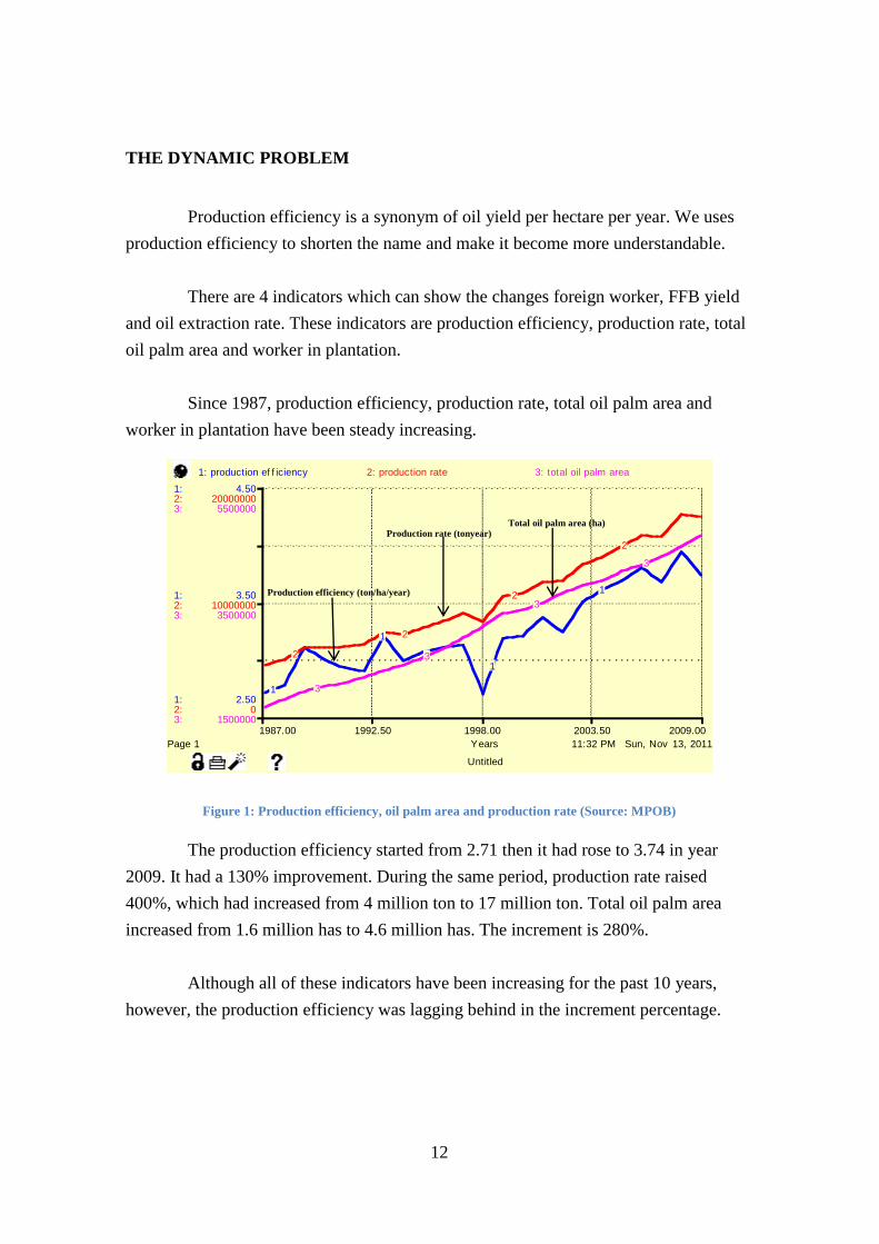
THE DYNAMIC PROBLEM
Production efficiency is a synonym of oil yield per hectare per year. We uses
production efficiency to shorten the name and make it become more understandable.
There are 4 indicators which can show the changes foreign worker, FFB yield
and oil extraction rate. These indicators are production efficiency, production rate, total
oil palm area and worker in plantation.
Since 1987, production efficiency, production rate, total oil palm area and
worker in plantation have been steady increasing.
Figure 1: Production efficiency, oil palm area and production rate (Source: MPOB)
The production efficiency started from 2.71 then it had rose to 3.74 in year
2009. It had a 130% improvement. During the same period, production rate raised
400%, which had increased from 4 million ton to 17 million ton. Total oil palm area
increased from 1.6 million has to 4.6 million has. The increment is 280%.
Although all of these indicators have been increasing for the past 10 years,
however, the production efficiency was lagging behind in the increment percentage.
11:32 PM Sun, Nov 13, 2011
Untitled
Page 1
1987.00 1992.50 1998.00 2003.50 2009.00
Years
1:
1:
1:
2:
2:
2:
3:
3:
3:
2.50
3.50
4.50
0
10000000
20000000
1500000
3500000
5500000
1: production ef f iciency 2: production rate 3: total oil palm area
1
1
1
1
2
2
2
2
3
3
3
3
Production rate (tonyear)
Production efficiency (ton/ha/year)
Total oil palm area (ha)

13
HYPOTHESIS
The system dynamics model describe in this section will give more dynamics
insight for the production, workforce recruitment and how these sector mutually
influence each other. The hypothesis will describe by using causal loop diagrams. The
discussion of the model will highlights the main feedbacks that we believe are
responsible for the system behaviour. Finally, the stock and flow structure of the model
is explained and focus on the delays and interaction between the model sectors.
Hypothesis overview
In 2009, production efficiency is about 3.7 ton per ha per year. In theory, the
production efficiency can reach 18.5 ton per ha per year (Dr. Yusof Basiron, 2006,
MPOC). The production efficiency is a ratio of production rate and total oil palm area
(Figure 1). Production efficiency is a measurement of utilization of land use.
There are 2 reasons we use production efficiency as an indicator. First,
production efficiency shows the relationship between palm oil production and land
usage. Second, production efficiency reflects the true nature of oil palm plantation. In
the extremely condition, increasing of production rate may be caused by larger
plantation area. Third, production efficiency decides the new plantation expansion
speed.
Figure 2: The factors influence production efficiency
total oil palm area
production
efficiency
production rate
+
-

14
CAUSAL LOOP DIAGRAM: CAPACITY SECTION
Capacity Section is about the plantation of oil palm area. There are three kinds
of oil palm areas: Immature oil palm area, high yield mature oil palm area and
deteriorated mature oil palm area.
PLANTATION CYCLE
New oil palm tree flows into immature oil palm area through a planting rate.
After a few years, immature oil palm area becomes high yield mature area. High yield
mature area can yield fresh fruit branch (FFB) used for oil extraction. When high yield
mature area is becoming older, it will go in deteriorated mature area. Deteriorated
mature area still can yield fresh fruit branch, but with a lower rate. When Deteriorated
mature area become older estate owner may clear cut the old oil palm tree. After clear
cut process, owner can replant new tree with a planting rate (R1, Figure 3). High
planting rate leads to increasing of oil palm area. Oil palm area then feedbacks to
planting rate.

15
Figure 3: Plantation cycle
CONTRIBUTION OF DETERIORATED AND HIGH YIELD AREA TO
PRODUCTION EFFICIENCY
Both high yield and deteriorated area can yield fresh fruit branch. From every
year, harvested fresh fruit branch can be used for oil extraction. The extracted oil is the
is production rate. Oil extraction rate (OER) is indicator of extraction efficiency.
Production rate then influences the production efficiency. Production efficiency has
negative impact on desired oil palm tree, because the production can be satisfied with
less capacity if the production efficiency is very high (C1,C2, Figure 4).
immature oil palm
area
high yield mature oil
palm area
deteriorated mature
oil palm area
total mature oil palm
tree area
total oil palm tree
area
+
+
+
+
total ffb per year
production
efficiency
production rate
+
-
+
+
++
+
planting rate
+
+
R1
density of agricultural
land for new oil palm tree
-
+
desired oil palm
tree
+
oil extraction rate
+

16
Figure 4 Contribution of deteriorated and high yield area to production efficiency
immature oil palm
area
high yield mature oil
palm area
deteriorated mature
oil palm area
total mature oil palm
tree area
total oil palm tree
area
+
+
+
+
total ffb per year
production
efficiency
production rate
+
-
+
+
++
+
planting rate
+
+
R1
density of agricultural
land for new oil palm tree
-
+
desired oil palm
tree
+
oil extraction rate
+
-
C2
C1

17
OIL PALM AREA RAISES PLANTING RATE
Total oil palm area is the sum of all oil palm area. Total oil palm area affects
production efficiency reversely. Increasing of oil palm area is decreasing of production
efficiency. In order to meet the demand of palm oil production, the desired oil palm tree
will be increased. The increment then feedback to total oil palm area. (R2,R3,R4,R5,
Figure 5).
Figure 5: Oil palm area raises planting rate
immature oil palm
area
high yield mature oil
palm area
deteriorated mature
oil palm area
total mature oil
palm area
total oil palm area
+
+
+
+
total ffb per year
production
efficiency
production rate
+
-
+
+
++
+
planting rate
+
+
R1
density of agricultural
land for new oil palm
-
+
desired oil palm
tree
+
oil extraction rate
+
-
C2
C1
R3
R4
R2

18
PRODUCTION SECTION
Production of palm oil relies on machine. The palm oil processing is quite
complicated, which included sterilization, threshing, digestion, pulp pressing, oil
clarification, oil drying, oil packing. However, the process time is very short, which
only takes a 48 hours to a few days. However, the model in the paper was used years as
measuring unit. Therefore, the disturbance from the processing will not surface, because
the measurement unit is very difference in scale and the bigger unit tends to pave the
disturbance. Because of this reason, the palm oil processing has been simplified. The
number of production is multiplication of fresh fruit branch and oil extraction rate.
Oil extraction rate (OER) was clearly defined .(Chang et al., oil palm Industry
economic journal, volume 3, 2003[9]). In paper, Chang define the Oil extract rate as
ratio of oil recovered and Fresh fruit branch (FFB) times 100. Mathematics formula is:
In the thesis, oil extraction rate is an average of machine performance. It measure how
well the machine can extract palm oil. Oil extraction rate affects production rate
positively (Figure 6).
Figure 6: Oil Extraction rate and production rate
production rate
oil extraction rate
+

19
WORKER SECTION
Production of Palm oil depends on fresh fruit branch, which can be harvested
through a mini tractor grabber or manual labour. Increasing of workforce through a hire
a rate will increase the tatal ffb haversting rate because of labour can collect more fresh
fruit. Increasing of fresh fruit will increase the production efficiency. The production
efficiency then reduces the desired oil palm area because the demand of palm oil can be
satisfied with smaller oil palm area. With smaller oil palm area, the demand of
workforce will be reduced (C3,Figure 5).
High desired workforce demand will increase the interest of using machine to
replace the worker. The workforce replacement will increase as the desired workforce.
Desired workforce increases the number of actual mini tractor grabber, which can
replace workforce partially (C4, R5, Figure 5).
Figure 7: Workforce can be replaced by mini tractor grabber
total oil palm area
total ffb per yearproduction
efficiency
production rate
+
+
planting rate
desired oil palm
area
+
oil extraction rate
+
-
desired workforce
workforce
replacement
gap of mini tractor
grabber
actual mini tractor
grabber
workforce from
grabber
ratio of actual and
desired workforce
+
+
+
+
+
gap of workerforce
+
hire rate +actual workforce +
+
-
+
+
+
C3
C4
R5

20
MODEL STRUCTURE
This section is focus on elaborating the logic behind structures. Some of the
important equations and model detail will be presented here.
The Model Boundary
The variables considered vital for understanding the oil palm system and the
interplay between production efficiency and performance of the Palm Oil system.
Endogenous Exogenous Excluded
new planting rate
desired replant rate
production efficiency
desired oil palm tree
clear cut delay
mature time
agriculture land bank
FFB yield per high yield
area per year
FFB yield per deteriorated
area per year
land acquire delay
average oil palm tree per
workers
domestic demand rate
export demand rate
grabber adjustment time
grabber life time
efficiency of grabber to
worker
efficiency of grabber to
worker
system feedback to export
demand
international palm oil price
influences to local market
government implement
new policies
environment influences on
oil palm growth rate and
yield rate.
oil palm trees density in
one hectare area
Table 3: List of variables
In the model, we did not include the cost of production. We also assume that
the demand of palm oil is mostly come from international. Malaysia domestic
consumption is very small. Therefore, the influence from domestic consumption and
feedback can be ignored.

21
Time Horizon
The oil palm tree production cycle is from 20 to 30 years. Depend on clear cut
delay which could take 1 year to 10 year. In other words, the minimum production cycle
is 20 years. We choose to run the model from 1987 to 2009 which is 22 years. The
reason is the data before 1987 either incomplete or inconsistent among different
authorities. Therefore, using these data is risky, unreliable and may lead to a wrong
conclusion.
The Stock and Flow Structures
The stock and flow structure will be described by subdividing. The stock and flow
structure will be described separately. Start with capacity modules, production modules
and workforce modules. We will describe from a simplified structure, and then proceed
further. The full stock and flow diagram is available in Appendix.

22
THE CAPACITY OIL PALM SECTION
Figure 8: Stock and flow diagram for oil palm capacity
The capacity for palm oil only consists of 3 stocks: Immature oil palm area,
high yield mature oil palm area and deteriorated oil palm area.
total oil palm area
planting rate
Immature oil palm area
deteriorated mature
oil palm area
mature rate
clear cut rate
deterioration rate
high y ield mature oil palm area
agriculture land bank
total mature oil palm tree area
clear cut delay
mature time
density of agricultural
land f or oil palm tree
FFB y ield per
deteriorated tree per y ear
FFB y ield per high
y ield per y ear
desired replant rate
new planting rate
FFB f rom deteriorated
area per y ear
FFB f rom high
y ield area per y ear
total FFB per y ear
production ef f iciency
deterorated time
land acquire delay

23
Each of the area represent the different age of oil palm tree grown in
plantation. We assume that the system is in equilibrium state that inflows equal to
outflows. With this assumption, we hypothesize that the plantation owner replants new
oil palm to the same plantation after a clear cut process. The desired replant rate
variable is the division of clear cut rate to density of agricultural land for oil palm tree.
It will add to planting rate as well as new planting rate. New planting rate influences by
the density of agriculture land. Density of agricultural land is represented in a
percentage form, which has a meaning of availability for oil palm tree. If it drops into
zero, there will be no more land for expansion.
New palm oil tree flows into immature oil palm area stock through a planting
rate. The planting rate influences by availability of land. The immature oil palm area
approximately takes 3 years, to become high yield mature. Only the mature oil palm
area can yield fresh fruit branch (FFB). The fresh fruit branch from high yield mature
area, is the multiplication of FFB yield per high yield area per year and the high yield
area.
The high yield area oil palm can stay in the stock for 17 year. During this
period, the oil palm area production is very high. Average fresh fruit branch yield per
hectare per year is about 23. After high yield period, it slowly change into deteriorated
mature oil palm area As high yield area, deteriorated mature oil palm area can also yield
fresh fruit branch, but with a lower rate of 18 yield per hectare per year in average. Both
high yield and deteriorated area are mature oil palm tree area.
The total oil palm area is the sum of immature and mature oil palm. The total
oil palm area influences the production efficiency reversely.
As we assume that the capacity of oil palm sector is in equilibrium state. If
there is no expansion of oil palm area, the immature, high yield and deteriorated area
should balance them self in a ratio of 3:17:5, according to the delay of each stock.

24
THE PRODUCTION SECTION
Figure 9: Production and production efficiency
The production efficiency is an indicator (Figure 7). It gauges the utilization of
land usage. High production efficiency means the production is very effective. The
reason we use production efficiency instead of production rate itself because the
production is misleading. Increasing of production could be the result of oil palm area
expansion. The formula of production efficiency is shown as follow:
The production section has no stock due to the reason we have stated in causal loop
diagram production section.
total oil palm area
total FFB per y ear
production ef f iciency
production rate
oil extract rate

25
THE WORKFORCE SECTION
Figure 10: Workforce section
The workforce section consists of two productive elements, which are manual
labour and machine. The upper stock, actual mini grabber is a machine which use for
replacement of workforce when suffering from labour shortage. Because of the terrain
limitation, the machine may not accessible to all terrain. This is the reason that manual
labour workforce still dominating the oil palm area. The lower stock, actual workforce
represents manual labour workforce (Figure 8).
We hypothesized workforce is decided by total oil palm area. This is
reasonable, as the larger area need more workers to manage. Worker is the workforce
that is needed to be allocated to harvest the fresh fruit branch. Using machine can
indeed replace labour, but using machine cannot reduce fruit harvesting task need to be
done.
The bottom left desired workforce is the total labour workforce needed. We
assume that each single unit of labour workforce carry single unit of workforce. The
leav ing rate
actual mini tractor grabber
gap of workf orce
grabber buy ing rate
ef f iciency of grabber to worker
grabber adjustment time
ratio of actual and
desired workf orce
actual workf orce
hire rate
hire time tenure ends time
av erage oil palm
area per worker
desired workf orce
workf orce replacement
worker dependency
grabber depreciation rate
gap of mini tractor grabber
total oil palm area
workf orce f rom grabber
grabber lif e time
efficiency of grabber to worker
desired mini tractor grabber

26
single unit of work force can be described as average oil palm area per worker. Desired
workforce has a reverse relationship to actual workforce. When there is a gap, labour
will flow into or out of actual workforce through a hire rate. The labour can be reduced
before tenure ends. In here, we assume that the hire time is 1 year. The tenure ends time
is 5 years which is decided by the government. The labour exit the stock with the
leaving rate will be replenished through hire rate, in order to stable the labour force.
This can be done because government allow plantation owner to replenish the labour
force, after the tenure ends. Worker dependency represents the dependency of labour
workforce. Worker dependency is a decision which influences the hire rate.
When there is a scarcity of workforce, especially labour shortage, estate owner
tends to search workforce replacement. The desired machine is called mini tractor
grabber. The desired mini tractor grabber creates a gap of mini tractor grabber that
eventually influences grabber buying rate. The adjustment time is 1 year. Through the
buying rate, the system builds up the stock of mini tractor grabber. However, one
should know that the grabber has a life time of 5 years. After 5 year, the owner may buy
new grabbers again. The grabber can increase the productivity for almost 1.25
percentage compare with manual labour. The actual and desired workforce will always
balance themselves so than the workforce can be fully utilized. Ratio of actual and
desired workforce represents utilization of workforce.

27
ANALYSIS
The model is a tool that allows us to understand the real world structure. But
the model cannot be as complex as the real world, otherwise the model will become too
complicated to be comprehend. Therefore, building a simplified model which merely
reflects the problem is the key. Through this, we may able to understand the
problematic behavior and to study the structure causes the problem.
The model has to be tested and make sure that it will produce predicted
behavior within a range of reasonable inputs. By testing the model, we may find out
some ambiguous structures in the model which generate unreasonable result. We have
to make sure that the model generates reasonable results. Then model will become
stable. If the model is stable, we will have confident in it.
With a stable model, we can begin to use it to study as well as to understand
our real structure effectively. The model running on a virtual environment can become a
test ground for different alternative strategies, so that the impact of the strategies can be
studied before implementation.
In this section, we will cover a few test designs to ensure the model is stable.
The model will divide into two main sections: Direct structure test and structure
orientated behavior test.
Direct structure test
The production section of the model is based on the descriptive data in
Malaysia Palm Oil Board2, wikipedia3 website and Malaysia Felda holding4
previously an government agency.
The production structure is based on Food and Agriculture Organization of the
United Nations5 which describe the process of oil processing in detail.
The workforce structure is based on the description on The Malaysia Palm Oil
Cluster Final Report6
2 http://www.mpob.gov.my/ 3 http://en.wikipedia.org/wiki/Oil_palm 4 http://www.felda.net.my/feldav3/ 5 PALM OIL PROCESSING, http://www.fao.org/DOCREP/005/Y4355E/y4355e04.htm 6 http://www.isc.hbs.edu/pdf/Student_Projects/Malaysia_Palm_Oil_2011.pdf

28
The detail has been described in literature review, causal loop section and stock
and flow section, which the structure is a simplified version of real oil palm industry.
The new planting rate is based the gap between oil production rate and export demand.
Oil yield rate decides the number of new oil palm number than need to be planted.
Equilibrium shock test
The whole model was put into equilibrium state. By applying a sudden shock
of 250 extra export demand after year 1995, the decided export rate raise until 500. At
same moment the production efficiency fell slowly. From a value of 3.84, production
efficiency dropped until a value of 3.82. Production efficiency slowly climbed back to
equilibrium state approximately after 20 year.

29
Figure 11: Production efficiency response to shock input
The falling of production efficiency is the system immediately responses to the
sudden increase of export outflow. The decided export rate increases desired total
consumption rate.
In order to fulfill the desire consumption rate, the system will increase new
planting rate. The new planting rate increases immature oil palm area stock. The
Immature oil palm area will take 3 years to become mature tree which can produce
palm fruits that can be extracted for palm oil.
However, during the immature period, total oil palm tree stock has been
increased. Thus, the production efficiency is lower because immature oil palm area
cannot produce any palm fruit. The next section, we will test equilibrium shock reaction
by cutting out individual loops. The loop cutting test will be presented in 2 sections:
The capacity section and workforce section. In each section the loop cutting test has
been conducted differently.
8:48 AM Tue, Nov 15, 2011
Untitled
Page 1
1987.00 1992.50 1998.00 2003.50 2009.00
Years
1:
1:
1:
2:
2:
2:
4
4
4
200
350
500
1: production ef f iciency 2: export demand rate
1 1
1
1
2 2
2 2
3.82 250
3.69
500

30
Capacity Section
CUTTING C1 LOOP
C1 loop is reinforcing loop which always strengthen the effect of the loop. By
Cutting C1 loop, we break the link between new planting rate and immature oil palm
area after the sudden shock. The production efficiency was raises because new planting
rate.
If our hypothesis matches what we describe on C1 loop, cutting the C1 loop
will reduce the production efficiency (Figure 10).
Figure 12: Cutting C1
9:02 AM Tue, Nov 15, 2011
Untitled
Page 1
1987.00 1992.50 1998.00 2003.50 2009.00
Years
1:
1:
1:
3.795
3.825
3.855
production ef f iciency : 1 - 2 -
1 1
1
1
2 2
2
2
Before cutting C1
After cutting C1

31
CUTTING C2 LOOP
C2 are similar to C1 loop. It is reinforcing loop. By Cutting C1 loop, we should
able to observer behavior similar to C1. It bounced back because of the C1 loop still
running when C2 loop has been cut.
Figure 13: Cutting C2
CUTTING R2 LOOP
R2 is reinforcing loop. By cutting R2, the production efficiency should
increase because it reduces the unproductive immature oil palm area from total oil palm
area. The total oil palm area has a reverse relationship to productive efficiency.
Figure 14: Cutting R2
9:17 AM Tue, Nov 15, 2011
Untitled
Page 1
1987.00 1992.50 1998.00 2003.50 2009.00
Years
1:
1:
1:
3.825
3.84
3.855
production ef f iciency : 1 - 2 -
1 1
1
1
2 2
2
2
9:40 AM Tue, Nov 15, 2011
Untitled
Page 1
1987.00 1992.50 1998.00 2003.50 2009.00
Years
1:
1:
1:
3
4
5
production ef f iciency : 1 - 2 -
1 1
1
1
2 2
2
2
Before cutting C2
After cutting C2
Before cutting R2
After cutting R2

32
CUTTING R3 LOOP
R3 is reinforcing loop. By cutting R3, the production efficiency should
increase because it reduces the total oil palm area which has a reverse relationship to
productive efficiency.
Figure 15: Cutting R3
CUTTING R4 LOOP
Similar to R3, cutting R4 should increase the production efficiency.
Figure 16: Cutting R4
9:46 AM Tue, Nov 15, 2011
Untitled
Page 1
1987.00 1992.50 1998.00 2003.50 2009.00
Years
1:
1:
1:
3
5
7
production ef f iciency : 1 - 2 -
1 1
1
1
2 2 2
2
9:53 AM Tue, Nov 15, 2011
Untitled
Page 1
1987.00 1992.50 1998.00 2003.50 2009.00
Years
1:
1:
1:
3
4
5
production ef f iciency : 1 - 2 -
1 1
1
1
2 2
2
2
Before cutting R3
After cutting R3
Before cutting R4
After cutting R4

33
Workforce Section
CUTTING C3 LOOP
Cutting C3 has no effect to production efficiency. The shock increases the
desired workforce. However, cutting C3 loop, the actual workforce is not going to
response to the shock. The workforce demand, switch to mini tractor grabber through
workforce replacement. Therefore, mini tractor increases, while actual workforce
remains unchanged. Workforce influences FFB harvesting directly, when workforce
remain unchanged, production efficiency will not response to it.
Figure 17: Cutting C3
Figure 18: Cutting C3: Increasing of mini tractor grabber
10:04 AM Tue, Nov 15, 2011
Untitled
Page 1
1987.00 1992.50 1998.00 2003.50 2009.00
Years
1:
1:
1:
3.05
3.45
3.85
production ef f iciency : 1 - 2 -
1 1
1
1
2 2
2
2
10:36 AM Tue, Nov 15, 2011
Untitled
Page 1
1987.00 1992.50 1998.00 2003.50 2009.00
Years
1:
1:
1:
0
1000
2000
actual mini tractor grabber: 1 - 2 -
1 1
1
1
2 2
2
2
Before cutting C3
After cutting C3

34
Figure 19: Cutting C3: Unchanging actual workforce
CUTTING C4 LOOP
C4 loop is very similar to C3 loop. Cutting C4 loop will leave the workforce
demand to C3 loop. C4 is loop is almost identical to C3. Therefore, production
efficiency remained unchanged.
Figure 20: Cutting C4: Unchanging actual workforce
10:36 AM Tue, Nov 15, 2011
Untitled
Page 1
1987.00 1992.50 1998.00 2003.50 2009.00
Years
1:
1:
1:
750
1200
1650
actual workf orce: 1 - 2 -
1 1
1
1
2 2 2 2
10:46 AM Tue, Nov 15, 2011
Untitled
Page 1
1987.00 1992.50 1998.00 2003.50 2009.00
Years
1:
1:
1:
3.05
3.45
3.85
production ef f iciency : 1 - 2 -
1 1
1
1
2 2
2
2
Before cutting C3
After cutting C3

35
Figure 21: Cutting C4: Unchanging actual workforce
10:46 AM Tue, Nov 15, 2011
Untitled
Page 1
1987.00 1992.50 1998.00 2003.50 2009.00
Years
1:
1:
1:
0
250
500
actual mini tractor grabber: 1 - 2 -
1 1
1
1
2 2
2
2
Before cutting C3
After cutting C3

36
Sensitivity analysis
MATURE TIME
Mature time is the time that immature oil palm area becomes high yield mature
area. Through cutting C1, C2, R3, R4 loops test, we believe that longer mature time will
lead to poor performance of production efficiency (Figure 19). Longer mature time not
only reduces the production efficiency, but it also increases the time for production
efficiency restore back to its equilibrium state.
Figure 22: Long mature time poor performance
FFB YIELD PER HIGH YIELD AREA PER YEAR
FFB yield per high yield area per year is productivity indicator for oil palm
tree. It can only be changed by using new breed of oil palm tree. From cutting C1 loop,
we have realized that this variable may be responsible for the production efficiency.
From the test, we have discovered this variable is very sensitive to production efficiency
(Figure 20).
11:25 AM Tue, Nov 15, 2011
Untitled
Page 1
1987.00 1992.50 1998.00 2003.50 2009.00
Years
1:
1:
1:
3
4
5
production ef f iciency : 1 - 2 - 3 -
1 1
1
1
2 2
2
2
3 3
3
3
mature time =1
mature time = 2 mature time = 3

37
Figure 23: FFB yield in high yield area per year vs production efficiency
FFB YIELD PER DETERIORATED AREA PER YEAR
FFB yield per deteriorated area per year is similar to FFB yield per high yield
area per year. We believe that this variable share the similar characteristics as FFB yield
per high yield per year (Figure 21). This variable is not as sensitive as FFB yield per
high yield area per year.
Figure 24: FFB yield in deteriorated area per year vs production efficiency
11:35 AM Tue, Nov 15, 2011
Untitled
Page 1
1987.00 1992.50 1998.00 2003.50 2009.00
Years
1:
1:
1:
2.5
3.5
4.5
production ef f iciency : 1 - 2 - 3 -
1 1
1
1
2 2
2
2
3 3
3
3
12:43 PM Tue, Nov 15, 2011
Untitled
Page 1
1987.00 1992.50 1998.00 2003.50 2009.00
Years
1:
1:
1:
3.05
3.5
3.95
production ef f iciency : 1 - 2 - 3 -
1 1
1
1
2 2
2
2
33
3
3
FFB yield per high yield = 21 (ton/ha/year)
FFB yield per high yield = 23 (ton/ha/year)
FFB yield per high yield = 25 (ton/ha/year)
FFB yield per high yield = 18
(ton/ha/year)
FFB yield per high yield = 19
(ton/ha/year)
FFB yield per high yield = 20 (ton/ha/year)

38
OIL EXTRACTION RATE
Oil extraction is a variable directly affects production efficiency. Oil extraction
rate directly influences the production rate. And the production rate has a positive
relationship with production efficiency. From the testing we determine production
efficiency is sensitive to oil extraction.
Figure 25: Oil extraction rate
Simulation settings
The simulator is ithink v9.14.
DT set to 0.25
Time measurement unit is year
Runge Kutta integration method was chosen to ensure accuracy result.
Simulation start from 1987 to 2009.
1:10 PM Tue, Nov 15, 2011
Untitled
Page 1
1987.00 1992.50 1998.00 2003.50 2009.00
Years
1:
1:
1:
3
4
5
production ef f iciency : 1 - 2 - 3 -
1 1
1
1
2 2
2
2
3 3
3
3
Oil extraction rate = 21%
Oil extraction rate = 22%
Oil extraction rate = 23%

39
Recreation of reference mode
Recreation of reference mode is very essential. In this section we compared the
reference mode with the historical data so that we can assess the gap between historical
and simulation behavior. Theil;s statistics test was use to access the differences, even
the bare eyes assessment had been conducted.
The stocks in the model were initialized with historical data. Some of the
stocks which historical data was absent, we tried to create initialize it by using estimate
data.
In this section, we recreate the reference mode with simulation setting. The
model was initialized with historical setting. Some of the data which absent from
historical data were replaced by estimated data. We would like to compare the behavior
of historical behavior with the simulation behavior by examining variable of interest.
Figure 26 was the simulation result. blue line is historical behavior and red line is
simulation.
Figure 26: Recreation of reference mode
By directly observation without calculation, the simulation behavior matched
the trend of historical behavior. Initial behavior tendency was similar to the historical
Both starting point of simulation and ending point of simulation matched the historical
data. Starting point matched the historical data because we initial the stocks with
historical data. The ending point matched the ending history data just by chance. The
noise of historical behavior was not be captured.
2:58 PM Tue, Nov 15, 2011
Untitled
Page 1
1987.00 1992.50 1998.00 2003.50 2009.00
Years
1:
1:
1:
2:
2:
2:
2.5
3.5
4.5
1: historical production ef f iciency 2: production ef f iciency
1
1
1
1
2 2
2
2
Simulation
Historical data

40
The historical and simulation behavior were found to match with each other.
Simulated and actual trajectories can be explained by using Theil’s Inequality Statistics
(Theil, 1966). Trajectories can be explained in bias, unequal variation and unequal co-
variation. The sum of bias, unequal variation and unequal co-variation should equal to
100%, if there are different between historical and simulation behavior. Historical and
simulation behavior were found with 7% of bias, 4% of unequal variation. Hence,
unequal co-variation is 89%. That means square error mainly arises from the point-by-
point differences. However, the point-by-point differences are not imposes a treat on the
validity of the model, as the purpose of the model is to understand the long term
dynamics of the production efficiency in low term.

41
Historical production rate and simulation production rate
Figure 27: Historical and simulation production rate
The simulation behavior was constantly lower than historical behavior.
However, the trend for simulation behavior is very similar to historical behavior. There
is a sharp fall in 1998, but the simulation did not catch this changes. This sharp fall
behavior was caused by Asia financial crisis in 1997. Malaysia oil palm industry is
export driven industry, almost 90% of palm oil export to other countries. When the
financial crisis hit Asia, the order from other countries decreased, as a result the
production of palm oil fell.
6:05 PM Tue, Nov 15, 2011
Untitled
Page 1
1987.00 1992.50 1998.00 2003.50 2009.00
Years
1:
1:
1:
2:
2:
2:
4503000
11116500
17730000
1: historical production rate 2: production rate
1
1
1
1
2
2
2
2
Simulation
Historical
42
Historical total oil palm area and simulation oil palm area
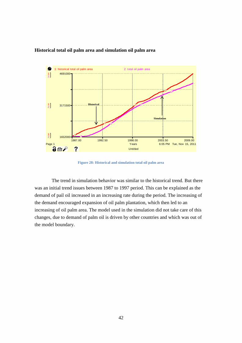
Figure 28: Historical and simulation total oil palm area
The trend in simulation behavior was similar to the historical trend. But there
was an initial trend issues between 1987 to 1997 period. This can be explained as the
demand of pail oil increased in an increasing rate during the period. The increasing of
the demand encouraged expansion of oil palm plantation, which then led to an
increasing of oil palm area. The model used in the simulation did not take care of this
changes, due to demand of palm oil is driven by other countries and which was out of
the model boundary.
6:05 PM Tue, Nov 15, 2011
Untitled
Page 1
1987.00 1992.50 1998.00 2003.50 2009.00
Years
1:
1:
1:
2:
2:
2:
1652000
3171500
4691000
1: historical total oil palm area 2: total oil palm area
1
1
1
1
2
2
2
2
Simulation
Historical

43
Figure 29: Reference mode reproduction
The simulation behaviors were not completely matched with the historical
behaviours. However, most of the behavior trends were similar to the historical trends.
For this, we believe that the model has already captured the dynamics problem from the
real world. The two factors: production rate and total oil palm area react together which
shape the production efficiency. The production efficiecny feedbacks to the system and
create the dyanmics problem. From the reference mode (Figure 29), production rate and
total oil palm area were react together, which generated fluctuation in production
efficiency.
6:58 PM Tue, Nov 15, 2011
Untitled
Page 1
1987.00 1992.50 1998.00 2003.50 2009.00
Years
1:
1:
1:
2:
2:
2:
3:
3:
3:
2.5
3.5
4.5
0
10000000
20000000
1500000
3000000
4500000
1: production ef f iciency 2: production rate 3: total oil palm area
1
1
1
1
2
2
2
2
3
3
3
3
production rate
total oil palm area
production efficiency

44
Reference mode: Sensitivity test
Previously shock test to the model shows that production efficiency is sensitive
to mature time, FFB yield per high yield area per year, and oil extraction rate. To
understand how these variables impact the reference mode. We will test these variables
separately.
MATURE TIME
The increasing of 1 year of mature time, it will leads to a fall of production
efficiency by 0.2. The behavior was expected as we conducted the shock test. The
behaviors were similar to each other. Longer time of mature time decreased the
production efficiency.
Figure 30: Mature time and reference mode
7:44 PM Tue, Nov 15, 2011
Untitled
Page 1
1987.00 1992.50 1998.00 2003.50 2009.00
Years
1:
1:
1:
2.5
3.5
4.5
production ef f iciency : 1 - 2 - 3 -
1
1
1
1
2
2
2
2
33
3
3
mature time = 3 (year)
mature time = 1 (year)
mature time = 2 (year)
45
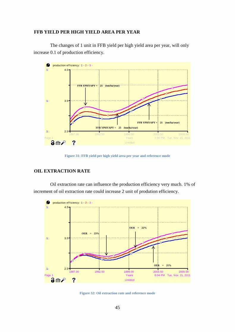
FFB YIELD PER HIGH YIELD AREA PER YEAR
The changes of 1 unit in FFB yield per high yield area per year, will only
increase 0.1 of production efficiency.
Figure 31: FFB yield per high yield area per year and reference mode
OIL EXTRACTION RATE
Oil extraction rate can influence the production efficiency very much. 1% of
increment of oil extraction rate could increase 2 unit of prodution efficiency.
Figure 32: Oil extraction rate and reference mode
7:56 PM Tue, Nov 15, 2011
Untitled
Page 1
1987.00 1992.50 1998.00 2003.50 2009.00
Years
1:
1:
1:
2.5
3.5
4.5
production ef f iciency : 1 - 2 - 3 -
1
1
1
1
22
2
2
3
3
3
3
8:04 PM Tue, Nov 15, 2011
Untitled
Page 1
1987.00 1992.50 1998.00 2003.50 2009.00
Years
1:
1:
1:
2.5
3.5
4.5
production ef f iciency : 1 - 2 - 3 -
1 1
1
1
22
2
2
33
3
3
FFB YPHYAPY = 21 (ton/ha/year)
FFB YPHYAPY = 25 (ton/ha/year)
FFB YPHYAPY = 23 (ton/ha/year)
OER = 21%
OER = 23%
OER = 22%

46
POLICY
After consideration two policies was proposed to improve the production
efficiency. Mature time was sensitive the system. But changing the mature time with
new breeding oil palm, in fact must take at less 26 years to complete a cycle. The policy
for mature time was considered not effective and was out of our purpose of achieving
significant result within 10 years.
We first elaborate and tested these policies. After that we conduct equilibrium
test on both policies separately. Finally, we test both polices together in scenario testing
section.
Policy Option 1
Allocating more workforce to high yield area. The policy directly increases the
fresh fruit branch production. Fresh fruit branch directly increases production rate. This
policy involves distribution of workforce.
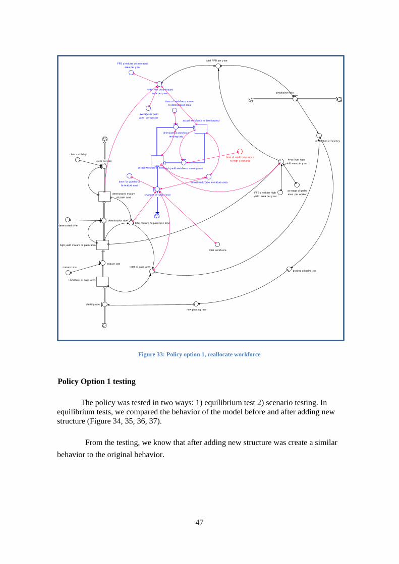
Analysis of Policy option 1
The main idea of this policy was allocating more workforce to the high yield
area, so that the efficiency in the high yield area can boast up greatly (Figure 33). This
policy doesn’t change the number of workforce as it involved just only distribution of
workforce.
This policy added two stocks which is actual workforce in deteriorated and
actual work force in high yield. Workforce in deteriorated area will move to high yield
area. However, workforce in high yield also moves back to deteriorated area. Usually
workforce will stay at high yield area and deteriorated area for a 17:5 ratio. If the ratio
increases, that means workforce will be concentrate to high yield area. Because of high
yield area can yield higher rate of fresh fruit per year. Therefore, increasing harvesting
activity in high yield area can boast up the production rate.
47
Figure 33: Policy option 1, reallocate workforce
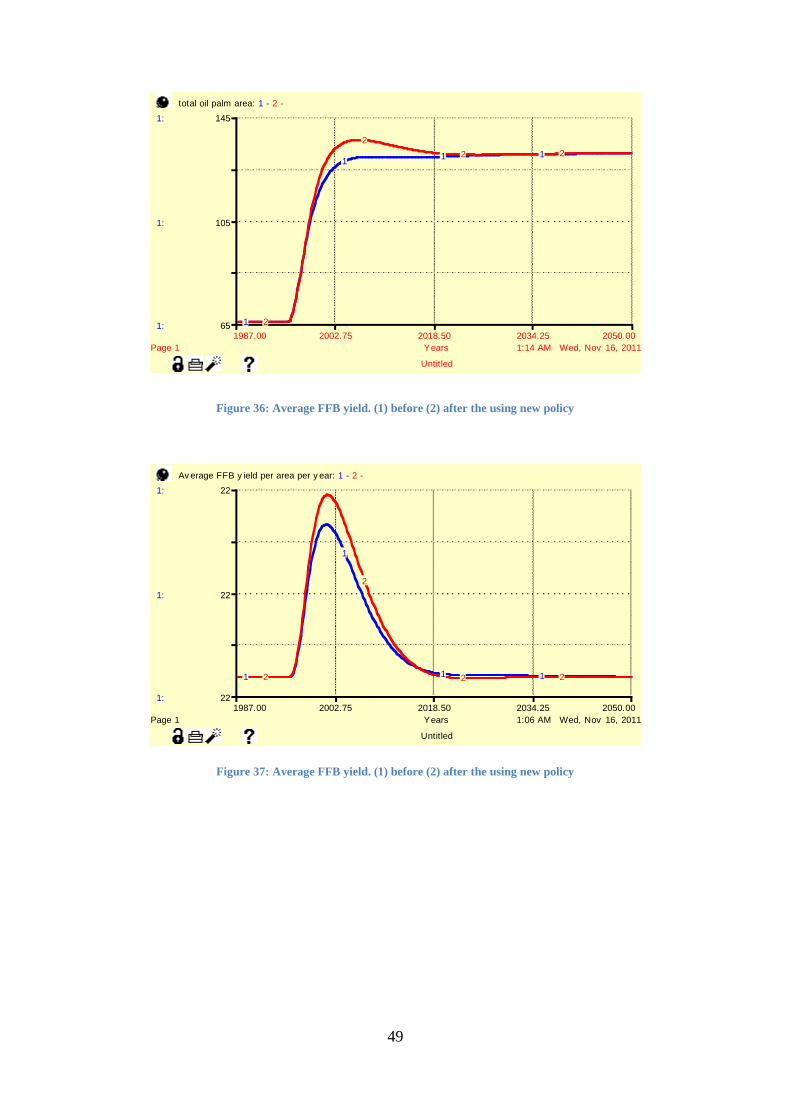
Policy Option 1 testing
The policy was tested in two ways: 1) equilibrium test 2) scenario testing. In
equilibrium tests, we compared the behavior of the model before and after adding new
structure (Figure 34, 35, 36, 37).
From the testing, we know that after adding new structure was create a similar
behavior to the original behavior.
total oil palm area
deteriorated mature
oil palm area
mature rate
clear cut rate
deterioration rate
high y ield mature oil palm area
total mature oil palm tree area
clear cut delay
mature time
FFB y ield per deteriorated
area per y ear
FFB y ield per high
y ield area per y ear
production rate
Immature oil palm area
FFB f rom deteriorated
area per y ear
FFB f rom high
y ield area per y ear
total FFB per y ear
production ef f iciency
new planting rate
deterorated time
planting rate
av erage oil palm
area per worker
actual workf orce in high y ield
deteriorated workf orce
mov ing rate
high y ield workf orce mov ing rate
time of workf orce mov e
to high y ield area
time of workf orce mov e
to deteriorated area
average oil palm
area per workeractual workf orce in deteriorated
changes of work f orce
actual workf orce in mature areatime f or workf orce
to mature area
total workf orce
desired oil palm tree

48
Figure 34: Production efficiency. (1) before (2) after the using new policy.
Figure 35: Production rate. (1) before (2) after the using new policy
1:00 AM Wed, Nov 16, 2011
Untitled
Page 1
1987.00 2002.75 2018.50 2034.25 2050.00
Years
1:
1:
1:
2.9
3.4
3.9
production ef f iciency : 1 - 2 -
1
1
1 12
2
2 2
1:06 AM Wed, Nov 16, 2011
Untitled
Page 1
1987.00 2002.75 2018.50 2034.25 2050.00
Years
1:
1:
1:
200
400
600
production rate: 1 - 2 -
1
1
1 1
2
2 2 2
49
Figure 36: Average FFB yield. (1) before (2) after the using new policy
Figure 37: Average FFB yield. (1) before (2) after the using new policy
1:14 AM Wed, Nov 16, 2011
Untitled
Page 1
1987.00 2002.75 2018.50 2034.25 2050.00
Years
1:
1:
1:
65
105
145
total oil palm area: 1 - 2 -
1
11 1
2
2
2 2
1:06 AM Wed, Nov 16, 2011
Untitled
Page 1
1987.00 2002.75 2018.50 2034.25 2050.00
Years
1:
1:
1:
22
22
22
Av erage FFB y ield per area per y ear: 1 - 2 -
1
1
1 12
2
2 2
50
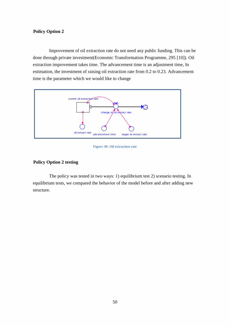
Policy Option 2
Improvement of oil extraction rate do not need any public funding. This can be
done through private investment(Economic Transformation Programme, 295 [10]). Oil
extraction improvement takes time. The advancement time is an adjustment time, In
estimation, the investment of raising oil extraction rate from 0.2 to 0.23. Advancement
time is the parameter which we would like to change
Figure 38: Oil extraction rate
Policy Option 2 testing
The policy was tested in two ways: 1) equilibrium test 2) scenario testing. In
equilibrium tests, we compared the behavior of the model before and after adding new
structure.
current oil extraction rate
change of oil extract rate
oil extract rateadv ancement time target oil extract rate
51
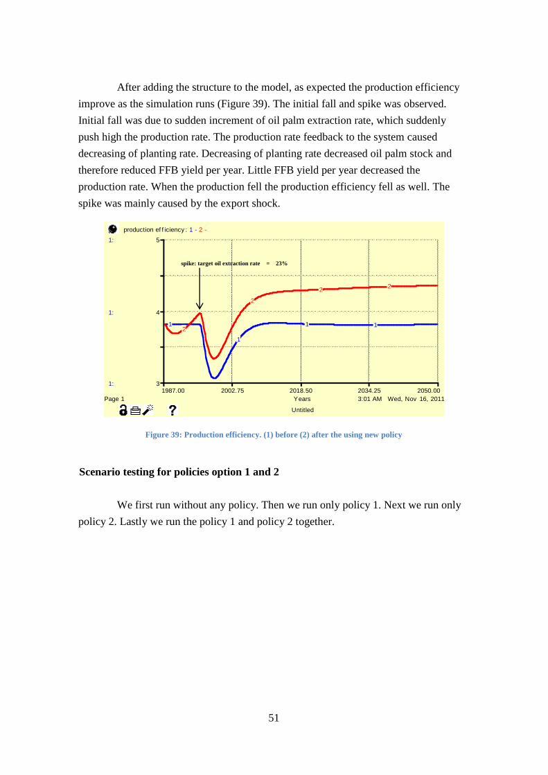
After adding the structure to the model, as expected the production efficiency
improve as the simulation runs (Figure 39). The initial fall and spike was observed.
Initial fall was due to sudden increment of oil palm extraction rate, which suddenly
push high the production rate. The production rate feedback to the system caused
decreasing of planting rate. Decreasing of planting rate decreased oil palm stock and
therefore reduced FFB yield per year. Little FFB yield per year decreased the
production rate. When the production fell the production efficiency fell as well. The
spike was mainly caused by the export shock.
Figure 39: Production efficiency. (1) before (2) after the using new policy
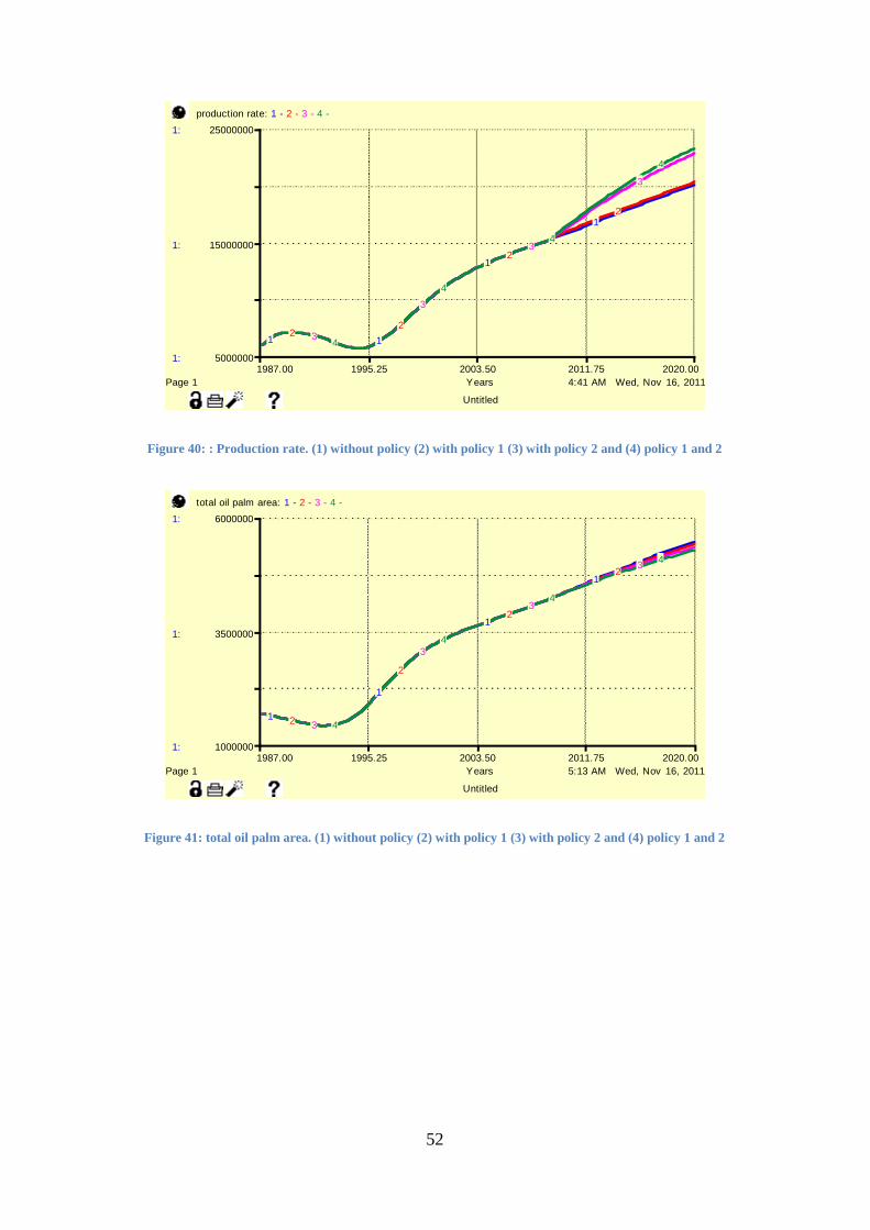
Scenario testing for policies option 1 and 2
We first run without any policy. Then we run only policy 1. Next we run only
policy 2. Lastly we run the policy 1 and policy 2 together.
3:01 AM Wed, Nov 16, 2011
Untitled
Page 1
1987.00 2002.75 2018.50 2034.25 2050.00
Years
1:
1:
1:
3
4
5
production ef f iciency : 1 - 2 -
1
1
1 12
2
22
spike: target oil extraction rate = 23%
52
Figure 40: : Production rate. (1) without policy (2) with policy 1 (3) with policy 2 and (4) policy 1 and 2
Figure 41: total oil palm area. (1) without policy (2) with policy 1 (3) with policy 2 and (4) policy 1 and 2
4:41 AM Wed, Nov 16, 2011
Untitled
Page 1
1987.00 1995.25 2003.50 2011.75 2020.00
Years
1:
1:
1:
5000000
15000000
25000000
production rate: 1 - 2 - 3 - 4 -
1 1
1
1
22
2
2
3
3
3
3
4
4
4
4
5:13 AM Wed, Nov 16, 2011
Untitled
Page 1
1987.00 1995.25 2003.50 2011.75 2020.00
Years
1:
1:
1:
1000000
3500000
6000000
total oil palm area: 1 - 2 - 3 - 4 -
1
1
1
1
2
2
2
2
3
3
3
3
4
4
4
4

53
Figure 42: Production efficiency. (1) without policy (2) with policy 1 (3) with policy 2 and (4) policy 1 and 2
Figure 43: : Actual workforce. (1) without policy (2) with policy 1 (3) with policy 2 and (4) policy 1 and 2
Through observation (Figure 40, 41, 42, 43) from the difference policy, we
were able to analyze and the behavior outcome.
Using Policy 1 separately we able the production indeed increase as expected.
We found that increasing of oil extraction rate doesn’t have help to reduce the number
of labor workforce (Figure 43). Even the productivity has been increased, but the total
oil palm area kept increasing. With the policies 1 and 2 combine, we can obtain a higher
production rate as well as production efficiency.
5:13 AM Wed, Nov 16, 2011
Untitled
Page 1
1987.00 1995.25 2003.50 2011.75 2020.00
Years
1:
1:
1:
2.5
4
5.5
production ef f iciency : 1 - 2 - 3 - 4 -
1
1
1 1
2
2
22
3
3
3
3
4
4
4
4
5:13 AM Wed, Nov 16, 2011
Untitled
Page 1
1987.00 1995.25 2003.50 2011.75 2020.00
Years
1:
1:
1:
100000
300000
500000
actual workf orce: 1 - 2 - 3 - 4 -
1
1
1
1
2
2
2
2
3
3
3
3
4
4
4
4
54
CONCLUSION
From our research, through the modeling process, we have learned the leverage
point of that responsible to the slow improvement of production efficiency. To resolve
the problem we have developed 2 policies, to improve the production efficiency,
through increasing fresh fruit branch yield in high yield area and oil extraction rate.
Fresh fruit branch yield in high yield area and extraction rate both play an
important role on increasing production rate. The delays of oil palm tree clear cut time
amazingly have weak relationship to production efficiency.
The workforce is not sensitive to the change of production efficiency. Mature
rate, high yield FFB yield per high yield area per year and oil extraction rate are
sensitive to production efficiency.
In term of supply and demand balance in oil palm system, actual workforce,
which represents the number of worker was not to be blame of low production
efficiency. As long as the plantation owner do not have willingness to switch from
manual labor workforce to mechanical method, the manual labor still remain the same
situation.

55
APPENDIX 1
Equations
actual_mini_tractor_grabber(t) = actual_mini_tractor_grabber(t - dt) + (grabber_buying_rate -
grabber_depreciation_rate) * dt
INIT actual_mini_tractor_grabber = initial_mini_tractor_grabber
INFLOWS:
grabber_buying_rate = (grabber_depreciation_rate*grabber_adjustment_time +
gap_of_mini_tractor_grabber)/grabber_adjustment_time
OUTFLOWS:
grabber_depreciation_rate = actual_mini_tractor_grabber/grabber_life_time
actual_workforce(t) = actual_workforce(t - dt) + (hire_rate - leaving_rate) * dt
INIT actual_workforce = initial_actual_estate_worker
INFLOWS:
hire_rate = ((gap_of_workforce)/hire_time ) + leaving_rate
OUTFLOWS:
leaving_rate = actual_workforce/tenure_ends_time
decided_oil_extraction_rate(t) = decided_oil_extraction_rate(t - dt) + (change_of_oil_extract_rate) * dt
INIT decided_oil_extraction_rate = initial_oil_extraction_rate
INFLOWS:
change_of_oil_extract_rate = (target_oil_extract_rate-decided_oil_extraction_rate) /advancement_time
desired_domestic_consumption_rate(t) = desired_domestic_consumption_rate(t - dt) +
(changing_of_domestic_consumption_rate) * dt
INIT desired_domestic_consumption_rate = domestic_demand_rate
INFLOWS:
changing_of_domestic_consumption_rate = MAX (0, ((domestic_demand_rate) -
desired_domestic_consumption_rate)/adjustment_time_of__domestic_consumption_rate )
desired_export_rate(t) = desired_export_rate(t - dt) + (change_of_export_rate) * dt
INIT desired_export_rate = export_demand_rate
INFLOWS:
change_of_export_rate = (export_demand_rate - desired_export_rate)/adjustment_time_of_desired_export_rate
deteriorated_mature_oil_palm_area(t) = deteriorated_mature_oil_palm_area(t - dt) + (deterioration_rate -
clear_cut_rate) * dt
INIT deteriorated_mature_oil_palm_area = initial_deteriorated_oil_palm_tree
INFLOWS:
deterioration_rate = high_yield_mature_oil_palm_area/deterorated_time
OUTFLOWS:

56
clear_cut_rate = deteriorated_mature_oil_palm_area/(clear_cut_delay )
domestic_stock(t) = domestic_stock(t - dt) + (production_rate - export_rate - domestic_consumption_rate) * dt
INIT domestic_stock = psychological_stock_level
INFLOWS:
production_rate = total_FFB_per_year*oil_extract_rate
OUTFLOWS:
export_rate = (desired_export_rate - adjustment_of_psycholigical_and_domestic_stock_level -
perceived_palm_oil_production_gap)
domestic_consumption_rate = (desired_domestic_consumption_rate)
high_yield_mature_oil_palm_area(t) = high_yield_mature_oil_palm_area(t - dt) + (mature_rate - deterioration_rate)
* dt
INIT high_yield_mature_oil_palm_area = initial_high_yield_oil_palm_tree
INFLOWS:
mature_rate = Immature_oil_palm_area/(mature_time)
OUTFLOWS:
deterioration_rate = high_yield_mature_oil_palm_area/deterorated_time
Immature_oil_palm_area(t) = Immature_oil_palm_area(t - dt) + (planting_rate - mature_rate) * dt
INIT Immature_oil_palm_area = initial_immature_oil_palm_tree
INFLOWS:
planting_rate = MAX (0, (desired_replant_rate + new_planting_rate)) *
density_of_agricultural_land_for_oil_palm_tree
OUTFLOWS:
mature_rate = Immature_oil_palm_area/(mature_time)
initial_base_real_price(t) = initial_base_real_price(t - dt)
INIT initial_base_real_price = historical_domestic_real_price
initial_max_total_potential_land_for_oil_palm(t) = initial_max_total_potential_land_for_oil_palm(t - dt)
INIT initial_max_total_potential_land_for_oil_palm =
initial_deteriorated_oil_palm_tree+initial_high_yield_oil_palm_tree+initial_immature_oil_palm_tree
Noname_19(t) = Noname_19(t - dt)
INIT Noname_19 = IF (l=1) THEN
desired_workforce * worker_dependency
ELSE
historical_worker_in_plantation
perceived_production_rate(t) = perceived_production_rate(t - dt) + (changing_of_production_rate) * dt
INIT perceived_production_rate = production_rate
INFLOWS:
changing_of_production_rate = (production_rate - perceived_production_rate)/adjustment_time_of_production_rate
shock_test_immature_oil_palm_tree(t) = shock_test_immature_oil_palm_tree(t - dt) + (shock_test_new_plant_rate -

57
shock_test_new_plant_exit_rate) * dt
INIT shock_test_immature_oil_palm_tree = 0
INFLOWS:
shock_test_new_plant_rate = if (time>=shocktestyear) then
if (is_cut_R2>0) then
new_planting_rate * density_of_agricultural_land_for_oil_palm_tree
ELSE
0
ELSE
0
OUTFLOWS:
shock_test_new_plant_exit_rate = shock_test_immature_oil_palm_tree/mature_time
adjustment_of_psycholigical_and_domestic_stock_level = (psychological_stock_level -
domestic_stock)/correction_adjustment_time
adjustment_time_of_desired_export_rate = 1
adjustment_time_of_production_rate = 1
adjustment_time_of__domestic_consumption_rate = 1
advancement_time = 20
agriculture_land_bank = IF (i=0) then
MAX (initial_max_total_potential_land_for_oil_palm,6600000 )
else
Round (initial_max_total_potential_land_for_oil_palm * 100)/100
agriculture_land_increment = 100
annually_salary_for_estate_worker = 1000 * 12
Average_FFB_yield_per_area_per_year = (FFB_from_high_yield_area_per_year +
FFB_from_deteriorated_area_per_year)
/ (
(FFB_from_high_yield_area_per_year/FFB_yield_per_high_yield__area_per_year)
+
(FFB_from_deteriorated_area_per_year/FFB_yield_per_deteriorated_area_per_year)
)
average_FFB_yield_per_year =
(FFB_yield_per_deteriorated_area_per_year+FFB_yield_per_high_yield__area_per_year)/2
average_oil_palm_area_per_mini_tractor_grabber = 25
average_oil_palm_area__per_worker = 12
base_real_price = initial_base_real_price
clear_cut_delay = 5

58
correction_adjustment_time = 1
cost_of_production_per_unit_FFB = 5200
density_of_agricultural_land_for_oil_palm_tree = (1-
(total_oil_palm_area/(agriculture_land_bank+agriculture_land_increment)))
desired_mini_tractor_grabber = workforce_replacement*efficiency_of_grabber_to_worker
desired_oil_palm_tree = IF (production_efficiency =0) THEN
0
ELSE
perceived_palm_oil_production_gap/production_efficiency
desired_replant_rate = IF (density_of_agricultural_land_for_oil_palm_tree=0) THEN
clear_cut_rate/1
ELSE
clear_cut_rate/density_of_agricultural_land_for_oil_palm_tree
desired_total_consumption_rate = desired_domestic_consumption_rate+desired_export_rate
desired_workforce = total_oil_palm_area/average_oil_palm_area__per_worker
deteriorated_palm_tree = FFB_yield_from_deteriorated/FFB_yield_per_deteriorated_area_per_year
deterorated_time = 17
domestic_demand_rate = IF (i = 0) THEN
+ (110000 * (TIME-STARTTIME) + 70000)
ELSE IF (j=1) THEN
v1 + STEP (v1 * percent_of_domestic_shock/100,shocktestyear)
ELSE
v1
efficiency_of_grabber_to_worker =
average_oil_palm_area__per_worker/average_oil_palm_area_per_mini_tractor_grabber
export_demand_rate = IF (i = 0) THEN
(540000* (TIME-STARTTIME) + 5500000 - 1000000 - 300000)
ELSE IF (j=1) THEN
v2 + STEP (v2 * percent_of_export_shock/100,shocktestyear)
ELSE
v2
FFB_from_deteriorated_area_per_year =
deteriorated_mature_oil_palm_area*FFB_yield_per_deteriorated_area_per_year
FFB_from_high_yield_area_per_year =
high_yield_mature_oil_palm_area*FFB_yield_per_high_yield__area_per_year

59
FFB_yield_from_deteriorated = initial_total_FFB_yield - FFB_yield_from_high_yield
FFB_yield_from_high_yield =
initial_total_FFB_yield*(ratio_of_FFB_rate_in_High_yield_and_FFB_rate_indeteriorated/(1+ratio_of_FFB_rate_in_
High_yield_and_FFB_rate_indeteriorated))
FFB_yield_per_deteriorated_area_per_year = 17
FFB_yield_per_high_yield__area_per_year = 23
gap_of_mini_tractor_grabber = desired_mini_tractor_grabber - actual_mini_tractor_grabber
gap_of_workforce = if (time<shocktestyear) then
( (desired_workforce ) - (actual_workforce / worker_dependency ))
else
( (desired_workforce ) - (actual_workforce / worker_dependency ))
grabber_adjustment_time = 1
grabber_life_time = 5
high_yield_palm_tree = FFB_yield_from_high_yield/FFB_yield_per_high_yield__area_per_year
hire_time = 1
i = IF (Is_equilibrium_test =1 OR Is_shock_test = 1) THEN
1
ELSE
0
immature_tree = high_yield_palm_tree/deterorated_time*mature_time
initial_actual_estate_worker = Noname_19
initial_average_real_price = 764.28
initial_deteriorated_oil_palm_tree = IF (l=1) THEN
deteriorated_palm_tree
ELSE
historical_mature_palm_oil_tree * share_of_deteriorated
initial_high_yield_oil_palm_tree = IF (l=1) THEN
high_yield_palm_tree
ELSE
historical_mature_palm_oil_tree *share_of_high_yield
initial_immature_oil_palm_tree = IF (l=1) THEN
immature_tree
ELSE
historical_immature_oil_palm_tree
initial_mini_tractor_grabber = max (0,desired_mini_tractor_grabber)
initial_oil_extraction_rate = IF (i >= 1) THEN
target_oil_extract_rate
60
ELSE
0.15
initial_stock_switch = 0
initial_total_consumption_rate = domestic_demand_rate+export_demand_rate
initial_total_FFB_yield = initial_total_consumption_rate / (target_oil_extract_rate)
is_cut_R2 = 0
Is_equilibrium_test = 0
Is_shock_test = 0
j = Is_shock_test
l = IF (i=1) THEN
1
ELSE
initial_stock_switch
land_acquire_delay = 2.5
mature_time = 3
minimum_supply_of_stock_in_year = 18/365
new_planting_rate = desired_oil_palm_tree/land_acquire_delay
Noname_9 = initial_total_FFB_yield * 0.2
oil_extract_rate = if (time >=2009) then
decided_oil_extraction_rate
else
decided_oil_extraction_rate - decided_oil_extraction_rate + 0.2
palm_oil_production_cost = 50
perceived_palm_oil_production_gap = (desired_total_consumption_rate - perceived_production_rate)
percent_of_domestic_shock = 100
percent_of_export_shock = 100
production_efficiency = IF (total_oil_palm_area=0) THEN
production_rate/total_oil_palm_area
ELSE
production_rate/total_oil_palm_area
production_efficiency_forecast = if (time >2009) then
historical_production_efficiency_2
else
historical_production_efficiency
production_rate_forecast = if (time >2009) then
historical_production_rate_2
else
historical_production_rate

61
psychological_stock_level = IF (i = 1) THEN
(perceived_production_rate) * minimum_supply_of_stock_in_year
ELSE IF (STARTTIME = TIME) THEN
historical_domestic_stock
ELSE
(perceived_production_rate) * minimum_supply_of_stock_in_year
ratio_of_actual_and_desired_workforce = if (time<shocktestyear) then
IF (desired_workforce = 0) THEN
0
ELSE
(actual_workforce + workforce_from_grabber) /desired_workforce
else
IF (desired_workforce = 0) THEN
0
ELSE
(actual_workforce + workforce_from_grabber) /desired_workforce
ratio_of_deteriorated_and_clear_cut = deterorated_time/clear_cut_delay
ratio_of_FFB_rate_in_High_yield_and_FFB_rate_indeteriorated =
ratio_of_deteriorated_and_clear_cut*ratio_of_FFB_yield_in_high_yield_and__FFB_yield_in_deteriorated
ratio_of_FFB_yield_in_high_yield_and__FFB_yield_in_deteriorated =
FFB_yield_per_high_yield__area_per_year/FFB_yield_per_deteriorated_area_per_year
refinary_cost = palm_oil_production_cost * total_FFB_per_year * oil_extract_rate
share_of_deteriorated = 1- share_of_high_yield
share_of_high_yield = deterorated_time/(clear_cut_delay + deterorated_time)
shocktestyear = 1995
target_oil_extract_rate = IF (i >= 1) THEN
0.2
ELSE
0.23
tenure_ends_time = 5
total_cost = (total_FFB_production_cost + refinary_cost-refinary_cost)
total_FFB_per_year = (FFB_from_deteriorated_area_per_year+FFB_from_high_yield_area_per_year) *
ratio_of_actual_and_desired_workforce
total_FFB_production_cost = cost_of_production_per_unit_FFB*total_FFB_per_year
total_mature_oil_palm_tree_area = high_yield_mature_oil_palm_area + deteriorated_mature_oil_palm_area
total_oil_palm_area =
Immature_oil_palm_area + total_mature_oil_palm_tree_area
total_oil_plam_area_and_forecast = if (time >2009) then

62
historical_total_oil_palm_area_2
else
historical_total_oil_palm_area
total_worker_cost = actual_workforce*annually_salary_for_estate_worker
v1 = 500
v2 = 500
worker_cost_and_total_cost = IF (total_worker_cost = 0) THEN
0
ELSE
total_cost/total_worker_cost
worker_dependency = 1
worker_forecast = if (time >2009) then
historical_worker_in_plantation_2
else
historical_worker_in_plantation
workforce_from_grabber = actual_mini_tractor_grabber /efficiency_of_grabber_to_worker
workforce_replacement = if (time<shocktestyear) then
Max (0, (desired_workforce - actual_workforce) )
else
Max (0, (desired_workforce - actual_workforce) )
historical_agriculture_land = GRAPH(TIME)
(1961, 4.2e+006), (1962, 4.3e+006), (1963, 4.3e+006), (1964, 4.4e+006), (1965, 4.4e+006), (1966, 4.5e+006), (1967,
4.5e+006), (1968, 4.6e+006), (1969, 4.6e+006), (1970, 4.7e+006), (1971, 4.7e+006), (1972, 4.8e+006), (1973,
4.8e+006), (1974, 4.9e+006), (1975, 4.9e+006), (1976, 5e+006), (1977, 5e+006), (1978, 5e+006), (1979, 5e+006),
(1980, 5.1e+006), (1981, 5.1e+006), (1982, 5.3e+006), (1983, 5.5e+006), (1984, 5.7e+006), (1985, 6e+006), (1986,
6.2e+006), (1987, 6.4e+006), (1988, 6.7e+006), (1989, 7e+006), (1990, 7.2e+006), (1991, 7.5e+006), (1992,
7.7e+006), (1993, 7.9e+006), (1994, 7.9e+006), (1995, 7.9e+006), (1996, 7.9e+006), (1997, 7.9e+006), (1998,
7.9e+006), (1999, 7.9e+006), (2000, 7.9e+006), (2001, 7.9e+006), (2002, 7.9e+006), (2003, 7.9e+006), (2004,
7.9e+006), (2005, 7.9e+006), (2006, 7.9e+006), (2007, 7.9e+006), (2008, 7.9e+006), (2009, 7.9e+006)
historical_domestic_consumption_rate = GRAPH(TIME)
(1980, 241951), (1981, 456616), (1982, 638867), (1983, 145000), (1984, 148879), (1985, 1e+006), (1986, 69812),
(1987, 118215), (1988, 542617), (1989, 1.2e+006), (1990, 414856), (1991, 984933), (1992, 463167), (1993,
1.9e+006), (1994, 565223), (1995, 1.4e+006), (1996, 1e+006), (1997, 1.7e+006), (1998, 568861), (1999, 1.6e+006),
(2000, 2e+006), (2001, 1.4e+006), (2002, 1.4e+006), (2003, 1.2e+006), (2004, 1.9e+006), (2005, 2.1e+006), (2006,
1.8e+006), (2007, 2e+006), (2008, 2.5e+006), (2009, 2.4e+006)
historical_domestic_Interest_rate_in_pecentage = GRAPH(TIME)
(1980, 8.50), (1981, 8.50), (1982, 8.50), (1983, 10.8), (1984, 12.2), (1985, 10.8), (1986, 10.0), (1987, 7.50), (1988,
7.50), (1989, 7.00), (1990, 6.99), (1991, 7.49), (1992, 8.68), (1993, 9.29), (1994, 8.22), (1995, 6.83), (1996, 8.03),

63
(1997, 9.18), (1998, 9.53), (1999, 10.6), (2000, 6.79), (2001, 6.79), (2002, 6.40), (2003, 6.40), (2004, 6.00), (2005,
6.25), (2006, 6.75), (2007, 6.75), (2008, 6.50), (2009, 5.55), (2010, 6.30), (2011, 6.30), (2012, 6.30), (2013, 6.30),
(2014, 6.30), (2015, 6.30), (2016, 6.30), (2017, 6.30), (2018, 6.30), (2019, 6.30), (2020, 6.30), (2021, 6.30), (2022,
6.30), (2023, 6.30), (2024, 6.30), (2025, 6.30), (2026, 6.30), (2027, 6.30), (2028, 6.30), (2029, 6.30), (2030, 6.30),
(2031, 6.30), (2032, 6.30), (2033, 6.30), (2034, 6.30), (2035, 6.30), (2036, 6.30), (2037, 6.30), (2038, 6.30), (2039,
6.30), (2040, 6.30), (2041, 6.30), (2042, 6.30), (2043, 6.30), (2044, 6.30), (2045, 6.30), (2046, 6.30), (2047, 6.30),
(2048, 6.30), (2049, 6.30), (2050, 6.30)
historical_domestic_price = GRAPH(TIME)
(1980, 919), (1981, 964), (1982, 829), (1983, 991), (1984, 1408), (1985, 1046), (1986, 579), (1987, 773), (1988,
1029), (1989, 822), (1990, 701), (1991, 837), (1992, 917), (1993, 890), (1994, 1284), (1995, 1473), (1996, 1192),
(1997, 1358), (1998, 2378), (1999, 1450), (2000, 997), (2001, 895), (2002, 1364), (2003, 1544), (2004, 1610), (2005,
1394), (2006, 1511), (2007, 2531), (2008, 2778), (2009, 2245)
historical_domestic_real_price = GRAPH(TIME)
(1980, 919), (1981, 879), (1982, 714), (1983, 823), (1984, 1125), (1985, 815), (1986, 449), (1987, 596), (1988, 791),
(1989, 616), (1990, 509), (1991, 583), (1992, 610), (1993, 572), (1994, 795), (1995, 882), (1996, 690), (1997, 766),
(1998, 1273), (1999, 756), (2000, 511), (2001, 453), (2002, 678), (2003, 759), (2004, 781), (2005, 656), (2006, 686),
(2007, 1127), (2008, 1173), (2009, 942)
historical_domestic_stock = GRAPH(TIME)
(1985, 342622), (1986, 342622), (1987, 278947), (1988, 575160), (1989, 765261), (1990, 424365), (1991, 456384),
(1992, 341795), (1993, 777941), (1994, 430024), (1995, 496497), (1996, 435414), (1997, 549549), (1998, 373733),
(1999, 717573), (2000, 905162), (2001, 734364), (2002, 589035), (2003, 594080), (2004, 890781), (2005, 892838),
(2006, 878551), (2007, 926979), (2008, 1.2e+006), (2009, 1.2e+006)
historical_harvasted_area = GRAPH(TIME)
(1975, 258204), (1976, 292093), (1977, 325210), (1978, 366293), (1979, 403898), (1980, 433146), (1981, 466280),
(1982, 505888), (1983, 545242), (1984, 592607), (1985, 626191), (1986, 671397), (1987, 1.2e+006), (1988,
1.4e+006), (1989, 1.5e+006), (1990, 1.6e+006), (1991, 1.6e+006), (1992, 1.7e+006), (1993, 1.8e+006), (1994,
1.9e+006), (1995, 2e+006), (1996, 2.1e+006), (1997, 2.3e+006), (1998, 2.3e+006), (1999, 2.6e+006), (2000,
2.6e+006), (2001, 2.7e+006), (2002, 2.8e+006), (2003, 2.9e+006), (2004, 3.1e+006), (2005, 3.2e+006), (2006,
3.3e+006), (2007, 3.8e+006), (2008, 3.9e+006), (2009, 3.9e+006)
historical_harvested_FFB = GRAPH(TIME)
(1975, 4.9e+006), (1976, 5e+006), (1977, 5.7e+006), (1978, 5.9e+006), (1979, 7.1e+006), (1980, 7.6e+006), (1981,
8.3e+006), (1982, 1e+007), (1983, 8.7e+006), (1984, 1.1e+007), (1985, 1.2e+007), (1986, 1.3e+007), (1987,
2.2e+007), (1988, 2.5e+007), (1989, 2.9e+007), (1990, 2.9e+007), (1991, 2.9e+007), (1992, 3e+007), (1993,
3.7e+007), (1994, 3.5e+007), (1995, 3.8e+007), (1996, 4e+007), (1997, 4.3e+007), (1998, 3.7e+007), (1999,
5e+007), (2000, 4.8e+007), (2001, 5.1e+007), (2002, 5.1e+007), (2003, 5.5e+007), (2004, 5.7e+007), (2005,
6.1e+007), (2006, 6.4e+007), (2007, 7.9e+007), (2008, 8.8e+007), (2009, 9e+007)
historical_immature_oil_palm_tree = GRAPH(TIME)
(1975, 256125), (1976, 260591), (1977, 260328), (1978, 249892), (1979, 268564), (1980, 245918), (1981, 259720),

64
(1982, 294178), (1983, 242161), (1984, 257815), (1985, 281389), (1986, 238732), (1987, 299728), (1988, 275017),
(1989, 274463), (1990, 283410), (1991, 267761), (1992, 307392), (1993, 285409), (1994, 267919), (1995, 297022),
(1996, 339139), (1997, 379906), (1998, 481170), (1999, 456692), (2000, 434873), (2001, 493745), (2002, 481936),
(2003, 498907), (2004, 424367), (2005, 419934), (2006, 461961), (2007, 540524), (2008, 572033), (2009, 615458)
historical_mature_palm_oil_tree = GRAPH(TIME)
(1975, 385666), (1976, 454009), (1977, 521486), (1978, 603087), (1979, 670299), (1980, 777388), (1981, 848143),
(1982, 888619), (1983, 1e+006), (1984, 1.1e+006), (1985, 1.2e+006), (1986, 1.4e+006), (1987, 1.4e+006), (1988,
1.5e+006), (1989, 1.7e+006), (1990, 1.7e+006), (1991, 1.8e+006), (1992, 1.9e+006), (1993, 2e+006), (1994,
2.1e+006), (1995, 2.2e+006), (1996, 2.4e+006), (1997, 2.5e+006), (1998, 2.6e+006), (1999, 2.9e+006), (2000,
2.9e+006), (2001, 3e+006), (2002, 3.2e+006), (2003, 3.3e+006), (2004, 3.5e+006), (2005, 3.6e+006), (2006,
3.7e+006), (2007, 3.8e+006), (2008, 3.9e+006), (2009, 4.1e+006)
historical_palm_oil_export_rate = GRAPH(TIME)
(1975, 1.2e+006), (1976, 1.3e+006), (1977, 1.4e+006), (1978, 1.5e+006), (1979, 1.9e+006), (1980, 2.3e+006), (1981,
2.5e+006), (1982, 2.9e+006), (1983, 2.6e+006), (1984, 3.2e+006), (1985, 3.4e+006), (1986, 4.6e+006), (1987,
4.2e+006), (1988, 4.3e+006), (1989, 5.2e+006), (1990, 5.7e+006), (1991, 5.6e+006), (1992, 5.6e+006), (1993,
6.1e+006), (1994, 6.8e+006), (1995, 6.5e+006), (1996, 7.2e+006), (1997, 7.5e+006), (1998, 7.5e+006), (1999,
8.9e+006), (2000, 9.1e+006), (2001, 1.1e+007), (2002, 1.1e+007), (2003, 1.2e+007), (2004, 1.3e+007), (2005,
1.3e+007), (2006, 1.4e+007), (2007, 1.4e+007), (2008, 1.5e+007), (2009, 1.6e+007)
historical_production_efficiency = GRAPH(TIME)
(1975, 1.96), (1976, 1.95), (1977, 2.06), (1978, 2.09), (1979, 2.33), (1980, 2.51), (1981, 2.55), (1982, 2.97), (1983,
2.41), (1984, 2.79), (1985, 2.79), (1986, 2.84), (1987, 2.71), (1988, 2.78), (1989, 3.11), (1990, 3.00), (1991, 2.93),
(1992, 2.90), (1993, 3.21), (1994, 2.99), (1995, 3.07), (1996, 3.11), (1997, 3.13), (1998, 2.70), (1999, 3.19), (2000,
3.21), (2001, 3.37), (2002, 3.24), (2003, 3.51), (2004, 3.61), (2005, 3.69), (2006, 3.81), (2007, 3.68), (2008, 3.95),
(2009, 3.74)
historical_production_efficiency_2 = GRAPH(TIME)
(2009, 3.74), (2010, 4.10), (2011, 4.30), (2013, 4.40), (2014, 4.47), (2015, 4.53), (2016, 4.58), (2018, 4.58), (2019,
4.60), (2020, 4.58)
historical_production_of_palm_oil_per_hectare = GRAPH(TIME)
(1975, 4.87), (1976, 4.77), (1977, 4.96), (1978, 4.87), (1979, 5.42), (1980, 5.94), (1981, 6.05), (1982, 6.94), (1983,
5.53), (1984, 6.27), (1985, 6.60), (1986, 6.77), (1987, 3.67), (1988, 3.64), (1989, 4.05), (1990, 3.90), (1991, 3.75),
(1992, 3.75), (1993, 4.09), (1994, 3.75), (1995, 3.90), (1996, 3.97), (1997, 4.00), (1998, 3.57), (1999, 4.11), (2000,
4.14), (2001, 4.43), (2002, 4.21), (2003, 4.58), (2004, 4.53), (2005, 4.66), (2006, 4.88), (2007, 4.20), (2008, 4.53),
(2009, 4.53)
historical_production_rate = GRAPH(TIME)
(1975, 1.3e+006), (1976, 1.4e+006), (1977, 1.6e+006), (1978, 1.8e+006), (1979, 2.2e+006), (1980, 2.6e+006), (1981,
2.8e+006), (1982, 3.5e+006), (1983, 3e+006), (1984, 3.7e+006), (1985, 4.1e+006), (1986, 4.5e+006), (1987,
4.5e+006), (1988, 5e+006), (1989, 6.1e+006), (1990, 6.1e+006), (1991, 6.1e+006), (1992, 6.4e+006), (1993,
7.4e+006), (1994, 7.2e+006), (1995, 7.8e+006), (1996, 8.4e+006), (1997, 9.1e+006), (1998, 8.3e+006), (1999,

65
1.1e+007), (2000, 1.1e+007), (2001, 1.2e+007), (2002, 1.2e+007), (2003, 1.3e+007), (2004, 1.4e+007), (2005,
1.5e+007), (2006, 1.6e+007), (2007, 1.6e+007), (2008, 1.8e+007), (2009, 1.8e+007)
historical_production_rate_2 = GRAPH(TIME)
(2009, 1.8e+007), (2010, 2e+007), (2011, 2e+007), (2013, 2.2e+007), (2014, 2.2e+007), (2015, 2.3e+007), (2016,
2.4e+007), (2018, 2.5e+007), (2019, 2.6e+007), (2020, 2.6e+007)
historical_total_oil_palm_area = GRAPH(TIME)
(1975, 641791), (1976, 714600), (1977, 781814), (1978, 852979), (1979, 938863), (1980, 1e+006), (1981, 1.1e+006),
(1982, 1.2e+006), (1983, 1.3e+006), (1984, 1.3e+006), (1985, 1.5e+006), (1986, 1.6e+006), (1987, 1.7e+006), (1988,
1.8e+006), (1989, 1.9e+006), (1990, 2e+006), (1991, 2.1e+006), (1992, 2.2e+006), (1993, 2.3e+006), (1994,
2.4e+006), (1995, 2.5e+006), (1996, 2.7e+006), (1997, 2.9e+006), (1998, 3.1e+006), (1999, 3.3e+006), (2000,
3.4e+006), (2001, 3.5e+006), (2002, 3.7e+006), (2003, 3.8e+006), (2004, 3.9e+006), (2005, 4.1e+006), (2006,
4.2e+006), (2007, 4.3e+006), (2008, 4.5e+006), (2009, 4.7e+006)
historical_total_oil_palm_area_2 = GRAPH(TIME)
(2009, 4.7e+006), (2010, 5.1e+006), (2011, 5.3e+006), (2012, 5.6e+006), (2013, 5.7e+006), (2014, 5.9e+006), (2016,
6.1e+006), (2017, 6.3e+006), (2018, 6.3e+006), (2019, 6.4e+006), (2020, 6.5e+006)
historical_worker_in_plantation = GRAPH(TIME)
(1975, 75975), (1976, 77459), (1977, 80947), (1978, 86634), (1979, 94990), (1980, 100963), (1981, 102373), (1982,
98106), (1983, 95237), (1984, 101493), (1985, 106539), (1986, 102976), (1987, 108470), (1988, 114681), (1989,
126498), (1990, 131842), (1991, 137140), (1992, 146369), (1993, 155295), (1994, 164808), (1995, 175427), (1996,
190183), (1997, 208646), (1998, 225100), (1999, 246088), (2000, 252549), (2001, 265182), (2002, 285444), (2003,
314658), (2004, 331648), (2005, 329709), (2006, 347755), (2007, 350000), (2008, 350000), (2009, 369000)
historical_worker_in_plantation_2 = GRAPH(TIME)
(2009, 369000), (2010, 382500), (2011, 395000), (2013, 410000), (2014, 430000), (2015, 442500), (2016, 467500),
(2018, 472500), (2019, 487500), (2020, 500000)

66
Appendix 2. Full Stock and flow diagram
Figure 44: Full stock and flow diagram for oil palm
total oil palm area
leaving rate
domestic stock
psychological stock level
actual mini tractor grabber
minimum supply of stock in year
perceived palm oil
production gap
planting rate
Immature oil palm area
deteriorated mature
oil palm area
mature rate
clear cut rate
deterioration rate
high yield mature oil palm area
agriculture land bank
total mature oil palm tree area
clear cut delay
mature time
density of agricultural
land for oil palm tree
desired oil palm tree
FFB yield per deteriorated
area per year
FFB yield per high
yield area per year
adjustment of psycholigical
and domestic stock level
perceived production rate
historical domestic stock
~
desired replant rate
new planting rate
production rate export rate
desired domestic
consumption rate
domestic consumption rate
oil extract rate
i
FFB from deteriorated
area per year
gap of workforce
FFB from high yield
area per year
total FFB per year
desired export rate
grabber buying rate
efficiency of grabber to worker
production efficiency
grabber adjustment time
domestic demand rate
export demand rate
deterorated time
ratio of actual and
desired workforce
change of export rate
desired total consumption rate
correction adjustment time
adjustment time of
desired export rate
changing of production rate
adjustment time of
production rate
actual workforce
changing of domestic
consumption rate
hire rate
adjustment time of
domestic consumption rate
hire time tenure ends time
average oil palm
area per worker
desired workforce
land acquire delay
workforce replacement
worker dependency
grabber depreciation rate
gap of mini tractor grabber
shocktestyearshocktestyear
agriculture land increment
workforce from grabber
grabber life time
efficiency of grabber to worker
desired mini tractor grabber

67
REFERENCES
1. Malaysia. Unit Pengurusan Prestasi dan P: Economic transformation
programme : a roadmap for Malaysia. Putrajaya: Performance Management
and Delivery Unit, Jabatan Perdana Menteri; 2010.
2. Elaine Lau Ying Man AB: A Qualitative Approach of Identifying Major Cost
Influencing Factors in Palm Oil Mills and the Relations towards Production
Cost of Crude Palm Oil. American Journal of Applied Sciences 8 (5): 441-446,
2011 2010.
3. Carter C, Finley W, Fry J, Jackson D, Willis L: Palm oil markets and future
supply. European Journal of Lipid Science and Technology 2007, 109(4):307-
314.
4. Basiron Y: Palm oil production through sustainable plantations. European
Journal of Lipid Science and Technology 2007, 109(4):289-295.
5. Abbai Belai DB, John Vrakas, Hashim Wasswa: The Malaysian Palm Oil
Cluster Final Report In.; 2011.
6. Emily B. Fitzherbert MJS, Alexandra Morel, Finn Danielsen, Carsten A. Bru¨ hl,
Paul F. Donald and Ben Phalan: How will oil palm expansion affect
biodiversity? Trends in Ecology and Evolution 2008, 23(10):545.
7. Ming KK, Chandramohan D: Malaysian palm oil industry at crossroads and its
future direction. Oil Palm Industry Economic Journal 2002, 2(2):10-15.
8. Jalani B, Basiron Y, Darus A, Chan K, Rajanaidu N: Prospects of elevating
national oil palm productivity: a Malaysian perspective. Oil Palm Industry
Economic Journal 2002, 2(2):1-9.
9. Chang LCARASaZB: An Economic Perspective of Oil Extraction Rate in the
Oil Palm Industry of Malaysia. OIL PALM INDUSTRY ECONOMIC
JOURNAL 2003, 3(1):30.
10. Economic transformation programme: a roadmap for Malaysia (1
Malaysia). In.: Performance Management and Delivery Unit (PEMANDU);
2010.