1

Impacts of Hydrological Uncertainty on Management of Water Resources 1

Newsha K. Ajami, George M. Hornberger, David L. Sunding, David N. Yates, and David 2

R. Purkey 3

Abstract 4

Improvement of techniques to assist in the sustainable management of water resource 5

systems is a crucial issue since our limited resources are under ever increasing pressure. 6

Water demand is on the rise because of growing population and increasing standards of 7

living. Water supplies, on the other hand, are being stressed by requirements for 8

improved water quality measures. Changes in the levels of water supply and demand 9

have increased the vulnerability of water-supply systems to shortfalls. This research 10

paper focuses on identifying and assessing impacts of end-to-end hydrological 11

uncertainty on efficient management of water-resources systems. We demonstrate an 12

Integrated Bayesian Uncertainty Estimator framework (IBUNE), which quantifies 13

uncertainty sources within the hydrological modeling process (including input forcing, 14

model parameters and model structural uncertainties). These uncertainty sources directly 15

affect streamflow predictions, and consequently water supply predictions. We propagate 16

these uncertainties through a water resources management and planning tool, WEAP, to 17

asses the impact of hydrological uncertainties on management of water resources. The 18

results of this study for the Upper Sacramento River of northern California, USA, suggest 19

that for reliable water resources management and planning, it is essential to account for 20

various sources of hydrological uncertainty. 21

2

1 INTRODUCTION 1

There is widespread recognition that an integrated approach to assess management 2

options for water-resources systems is necessary to inform the complex decisions facing 3

society today (e.g., Jakeman et al. 2006). In particular, it is essential that uncertainties in 4

environmental modeling be taken into account within the context of a risk-based 5

methodology (e.g., Maier and Ascough, 2006). One useful risk-based approach is to use 6

the concepts of reliability, resiliency, and vulnerability as proposed by Hashimoto et al. 7

(1982). Fowler et al. (2003) quantified the risk measures associated with each of these 8

concepts (reliability, resilience and vulnerability) in analyzing the impacts of climate 9

change on a catchment in England. 10

Economists have demonstrated the importance of hydrologic uncertainty in water 11

resource management, and have shown how such uncertainty affects the value of 12

property rights. The pioneering study of Burness and Quirk (1979) developed an 13

approach to water supply reliability that demonstrated how changes in the distribution of 14

water supply affects the value of access to water, and showed how legal institutions such 15

as water rights regimes can help users adapt to conditions of hydrologic uncertainty. Tsur 16

and Graham-Tomasi (1991) developed a similar model of water use that recognized the 17

buffering role of groundwater in determining the impact of water supply reliability. More 18

recently, papers by Howe et al. (1994) and Griffin and Mjelde (2000) have developed 19

applied models to capture the value of reliability in urban water systems, the latter paper 20

utilizing stated preference data to measure consumers' willingness to pay for a predictable 21

water supply. 22

3

A common approach to studying how hydrological variability affects water-supply 1

reliability is to use a historical sequence of measured hydrological variables (e.g., Brekke 2

et al., 2004; Cai and Rosegrant, 2004). This approach avoids the uncertainty introduced 3

from using a hydrological model, but is seriously limited by use of a relatively short 4

record and still suffers from an inherent measurement uncertainty. Another common 5

approach is to assign probabilities to different hydrological scenarios and study their 6

impact through economic analyses of water systems (e.g., Marques et al., 2005). 7

More recently, the inclusion of hydrological uncertainty estimates into integrated water 8

resources management modeling has focused primarily on input (forcing) variables (e.g., 9

Vicuna et al., 2007), for example to study impacts of climate change. These methods 10

ignore the importance of hydrological modeling uncertainty, which can play a significant 11

role on the accuracy of projected future events. 12

On the other hand, in the past decade some hydrologists have given much attention to 13

understanding and developing methods to estimate major sources of hydrological 14

modeling uncertainty (e.g. uncertainty associated with streamflow predictions or other 15

hydrological variables). Many studies have focused on hydrological uncertainties in 16

relation to parameter estimation (e.g. Beven and Binley, 1992; Kuczera and Parent, 1998; 17

Vrugt et al., 2003). Recently, a few studies have tried to address input (Kavetski et al., 18

2006a&b; Kuczera et al., 2006) and model structural (e.g. Vrugt et al., 2005) 19

uncertainties along with parameter uncertainties. As part of such efforts Ajami et al. 20

(2007) presented a Bayesian framework called Integrated Bayesian Uncertainty Estimator 21

4

(IBUNE), which incorporates model structure uncertainty along with uncertainty in 1

forcing variables and parameter values, into hydrological models. 2

Although input uncertainties have been treated (through climate change studies) within 3

water resources management models and although a full range of uncertainties have been 4

included in hydrological models, studies that investigate and address end-to-end impacts 5

of hydrological modeling uncertainties from a water-supply point of view (i.e., within a 6

management framework) are lacking. 7

In this study, we propose a methodology to quantify how uncertainty arising from the 8

hydrological modeling process propagates through a water resources management 9

system. We will investigate how these uncertainties translate into estimation of the 10

reliability, resilience, and vulnerability of a system. We evaluate the importance of the 11

uncertainty associated with hydrological input forcing, model parameter estimates, and 12

model structure. The sources of uncertainty in streamflow estimates are assessed using 13

IBUNE and the simulated streamflow ensembles are then propagated through a water 14

resources management and planning tool, WEAP (Water Evaluation and Planning; Yates 15

el al., 2005b), to evaluate the effect of hydrological uncertainty on water supply 16

predictions. We present the method in context, that is, in application to the watersheds 17

that contribute to the Shasta reservoir in the upper portion of the Sacramento river, 18

California, USA. The results indicate that accounting for different sources of 19

hydrological uncertainty will lead to more accurate streamflow predictions. Knowing a 20

full range of possible streamflow scenarios and their associated likelihood and 21

5

propagating them through a management tool, can provide valuable insights for decision 1

makers regarding the reliability and vulnerability of a water resources system. 2

2 METHODS 3

2.1 Assessment of hydrological uncertainty 4

To account for hydrological uncertainty we used the Integrated Bayesian Uncertainty 5

Estimator, (IBUNE; Ajami et al., 2007). IBUNE is a framework that accounts for three 6

major sources of uncertainty in hydrological predictions, including input (forcings), 7

model parameters, and model structural uncertainties. IBUNE combines and exploits the 8

strengths of an efficient and effective probabilistic parameter estimator algorithm and 9

Bayesian model combination technique, to provide an integrated assessment of 10

uncertainty propagating through the system. IBUNE works in two steps. First, it 11

estimates the uncertainty associated with input forcing (e.g. precipitation) and model 12

parameters for a set of hydrological models with different complexity levels. Since each 13

hydrological model is a simplified representation of real world processed, it can not 14

capture the entire physical behavior of the system. IBUNE reduces the model structural 15

deficiency by combining the simulated streamflow ensembles generated through different 16

hydrological models using Bayesian Model Averaging (BMA; Hoeting et al., 1999). The 17

combination weights are estimated based on the performance of the hydrological models 18

in capturing the observed behavior of the system. The final consensus hydrological 19

predictions reflect the uncertainty propagated through the system from the three major 20

sources. IBUNE results in both consensus deterministic and probabilistic hydrological 21

predictions. For more details on this framework reader is referred to Ajami et al. (2007). 22

6

2.2 Management model 1

Water Evaluation and Planning (WEAP) is an integrated hydrology and water resources 2

management model (Yates et al., 2005b). The model maintains equilibrium between 3

water supply (generated through watershed-scale hydrological processes) and various 4

water demands. At each time step, the network allocation is made, where criteria on 5

reservoirs and the distribution network and priorities and preferences of demands and 6

supplies determine the allocation according to maximization of demand “satisfaction”. 7

All flows are assumed to occur instantaneously, thus a demand site can withdraw water 8

from the river, consume some, optionally return the remainder to a wastewater treatment 9

plant and then return it to the river in the same time step. A monthly time step is typically 10

used but the model can be on daily, weekly, or even annual time steps. For more details 11

on WEAP model the reader is referred to Yates et al. [2005a&b]. The simulated 12

streamflow ensembles generated using IBUNE are propagated through WEAP to evaluate 13

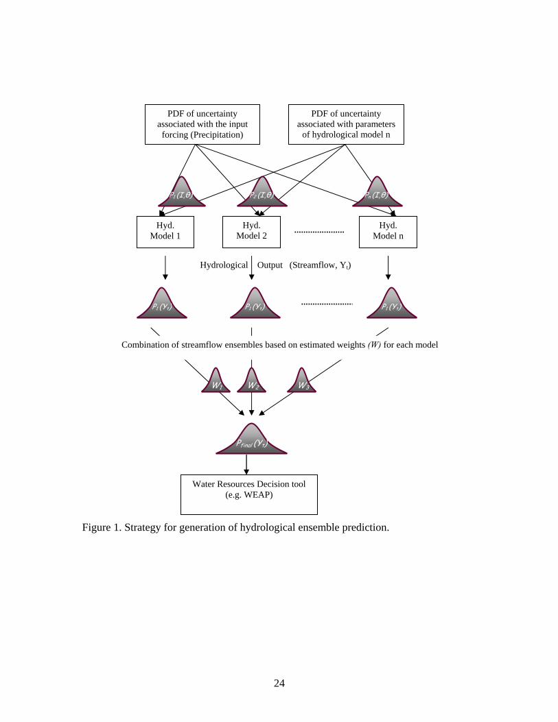
the effect of hydrological uncertainty on water supply predictions (Figure 1). 14

2.3 Reliability, resilience and vulnerability 15

Reliability, resilience and vulnerability are used here as indices to evaluate the 16

performance of a water resources system in meeting demand. These indicators were first 17

recommended by Hashimoto et al. [1982] and were later explored by Fowler et al. [2002] 18

to assess the performance of various water resources management systems under a 19

climate change scenario. First a criterion, C, is defined for the water supply sources, 20

where an unsatisfactory condition occurs when the specified demand is not met. The time 21

7

series of monthly demand coverage, Xt, are evaluated. If all the demand is met, we are in 1

a satisfactory (S) state, otherwise in an unsatisfactory (U) state [Hashimoto et al., 1982]: 2

Zt = (1) 3

An index, Wt, is defined to capture the transitions between satisfactory and unsatisfactory 4

states [Hashimoto et al., 1982]: 5

Wt = (2) 6

7

Now, if the periods of unsatisfactory state Xt are J1,…,JN then reliability, resilience and 8

vulnerability are defined as follows [Hashimoto et al., 1982; Fowler et al., 2002], where 9

T is the total number of elements in the time series: 10

Reliability T

ZT

tt∑

== 1RC (3) 11

Resilience ∑

∑

=

=

−= T

tt

T

tt

RS

ZT

WC

1

1 (4) 12

Vulnerability ⎭⎬⎫

⎩⎨⎧

=−= ∑∈

N....1i,XCmaxCiJt

tV (5) 13

Here, reliability, CR, measures the frequency of source failures to meet the specified 14

criterion (e.g. all the demand). Resilience, CRS, indicates the recovery speed of the system 15

1, if Xt∈U and Xt+1∈S 0, otherwise

1, if Xt∈S 0, if Xt∈U

8

from the state of failure. Vulnerability, CV, is a measure of the extent of failure. For more 1

details on these measures, the reader is referred to Hashimoto et al. [1982] and Fowler et 2

al. [2002]. 3

2.4 Study site and hydrological models 4

To make the application of the proposed method concrete and to develop quantitative 5

results, we used the watersheds that contribute to Shasta reservoir in the upper portion of 6

the Sacramento River, California (Figure 2). This upper portion of the watershed was 7

sub-divided into twelve sub-catchments that contribute to Shasta, with a monthly climate 8

time series derived from the 1/8 deg gridded daily time series computed as an average of 9

all grid cell values within the individual catchment (Maurer et al., 2002). Monthly 10

precipitation was given as the sum of the daily values for the period 1962 through 1994. 11

Other climate variables include temperature, wind speed and humidity each given as 12

monthly values for each catchment. The climatology of the Upper Sacramento River is 13

dominated by winter snowfall and dry, warm summers with little or no precipitation. 14

These climatological data were used as the forcing data for three different hydrological 15

models. These included the Sacramento Soil Moisture Accounting model (SAC-SMA, 13 16

parameters; Burnash et al., 1973), the Simple Water Balance model (SWB, five 17

parameters; Schaake et al., 1996) and the HYdrological MODel (HYMOD, five 18

parameters; Boyle, 2001). Parameters of SAC-SMA, HYMOD and SWB models are 19

listed in Tables (1), (2) and (3), respectively. We took the parameters of these three 20

models to be constant over the entire basin even though the models are spatially 21

distributed (12 sub-basins). 22

9

3 RESULTS 1

3.1 Probabilistic streamflow simulation 2

IBUNE’s estimated 95% uncertainty bounds (associated with input, model parameters 3

and model structural uncertainty), which are consistently narrow, capture most of the 4

observation points (Figure 3). The IBUNE framework, which optimally combines the 5

output of various hydrological models, clearly outperforms the individual models on both 6

the monthly Root Mean Square Error (RMSE) and monthly mean ABSolute Error 7

(ABSE) (Figure 4). 8

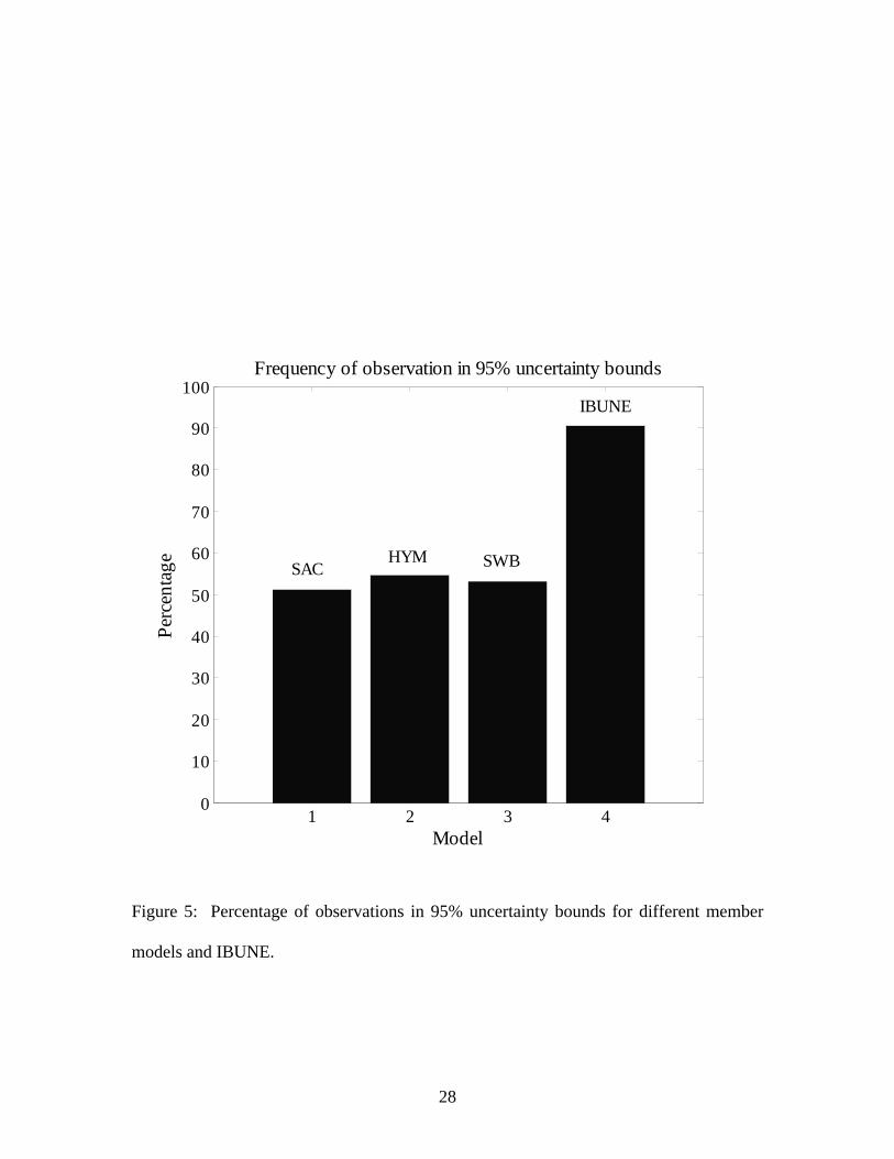
In addition to having relatively low error measures, a good model should have a posterior 9

distribution of errors that is consistent with the data. For example, approximately 95% of 10

the observation points should fall within the 95% forecast ranges (uncertainty bounds) of 11

a model. The individual hydrological models capture at most 55% of the observation 12

points, so they fail in this respect (Figure 5). However, as soon as we combine these 13

hydrological models to account for model structural uncertainty, the percentage of 14

observation points that fall within the uncertainty bounds increases to 90%. 15

3.2 Propagation of uncertainty through a water management system 16

After estimating the streamflow and its associated uncertainty using IBUNE, the 17

generated streamflow ensembles were used to force WEAP for demand projection under 18

the specified operational rules in the model. As a base of comparison the historical 19

observed streamflow was also fed into WEAP to asses the behavior of the water supply 20

10

system under the observed hydrological condition. Hereafter this scenario is called 1

observed. 2

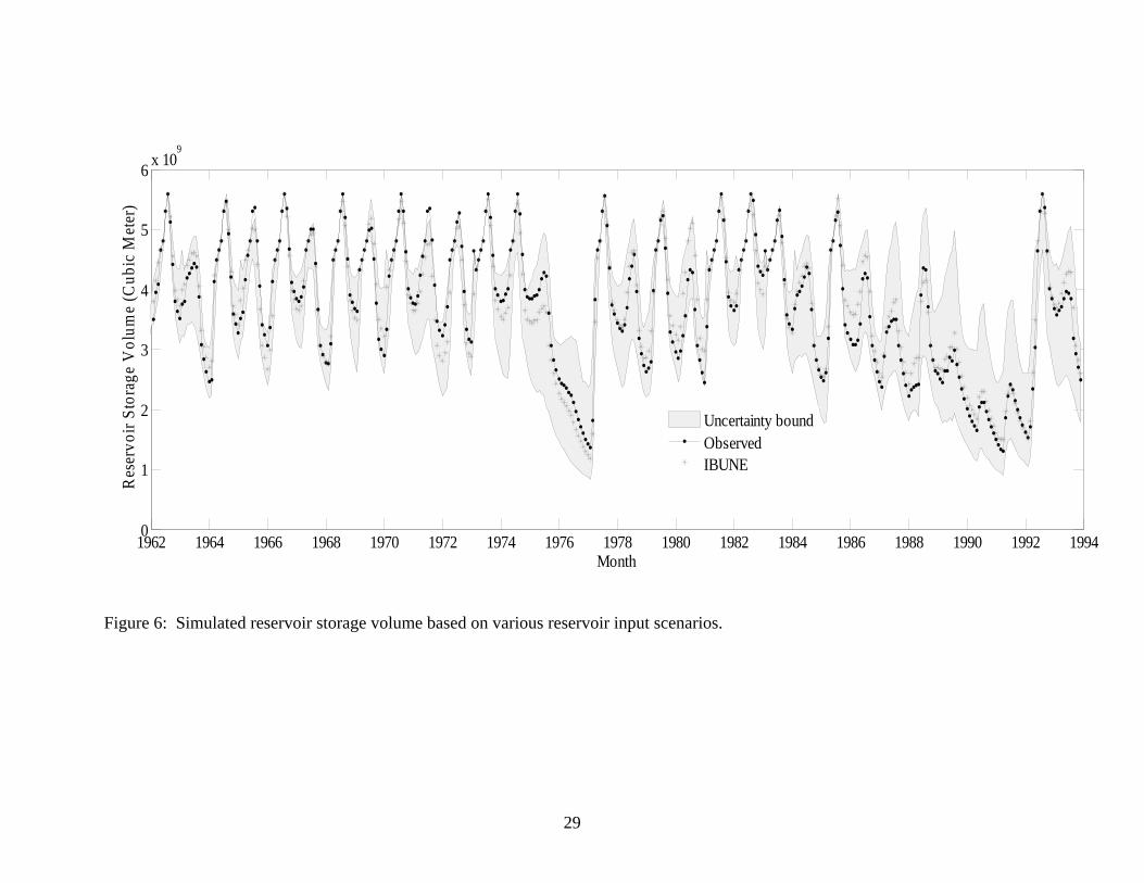
IBUNE simulations of storage volumes in Shasta compared reasonably well with 3

observed storage (Figure 6). This can be seen especially during the drought years of 1976 4

and 1977 and the dry period of 1989 through 1991. Also, we can see that as we 5

propagated the hydrological uncertainty through WEAP, the uncertainty bounds widen 6

(Figure 6) compared to streamflow (Figure 3). 7

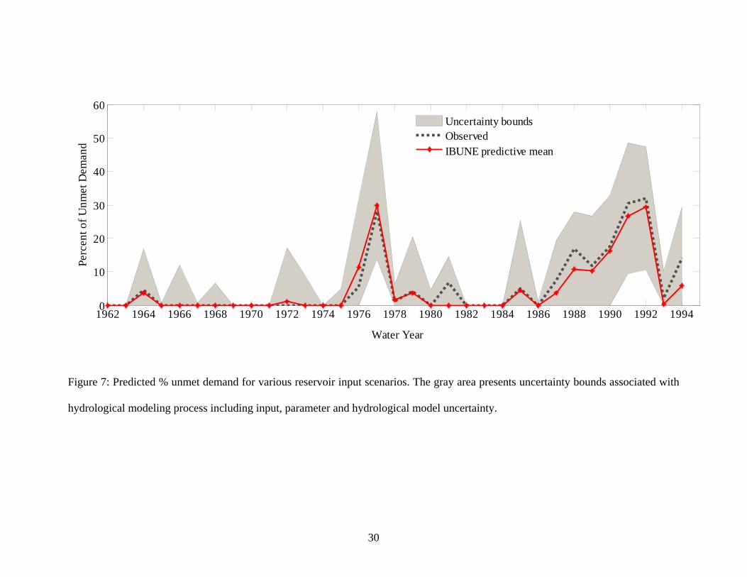
Percent of annual unmet demand was also studied (Figure 7). IBUNE performs quite 8

well in capturing the observed behavior of the system in meeting demand especially for 9

the drought years of 1976 and 1977. 10

3.3 Reliability, Resilience and Vulnerability 11

IBUNE’s predictive mean of unmet demand is found to be as reliable, to be more 12

resilient, and to be as vulnerable as observed unmet demand (Figure 8). This result 13

confirms the accuracy of IBUNE in matching the observed behavior of the system. 14

Having a good measure of reliability, resilience and vulnerability for different streamflow 15

scenarios provides vital information to decision makers. 16

For a 20% decline in reliability (lower bound in Figure 8), suddenly the system becomes 17

significantly (65%) more vulnerable compared to the mean behavior. This can be caused 18

by pre-specified operational rules within the model. These rules can be modified by the 19

decision makers to prevent high vulnerability. 20

11

Also looking at the annual RRV measures (T is equal to 12 in equations 4, 5 and 6), we 1

found that the system is significantly vulnerable to a sudden and considerable decline in 2

reliability, especially if it is during the drought period (Figure 9, lower bound scenario in 3

water year 1977). 4

4 DISCUSSION 5

Our results for hydrograph simulation using IBUNE show that it is crucial to account for 6

various sources of hydrological uncertainty. The consensus ensemble has superior 7

statistical properties (e.g. 40% more observation point falls within the 95% uncertainty 8

bounds) relative to the individual hydrological models (Figures 4 and 5). This result is 9

consistent with evaluations in other scientific areas (e.g., Jones et al. 2007). Araujo and 10

New (2007) have argued that robust models with a sensible estimate of uncertainty are 11

essential for guiding policy decisions related to potential ecological changes and that 12

ensemble forecasting is an excellent approach for providing such information. Our results 13

indicate that the same can be said for hydrological models. 14

When we propagated the uncertainty from IBUNE hydrology through Shasta Lake, the 15

width of the uncertainty bounds, especially during dry periods, increased (Figure 6). This 16

widening is mainly caused by the operational rules. Reservoir storage at the end of each 17

month depends on the water released from the dam, which is a function of demand, 18

inflow to the reservoir in that month, and the initial storage. In wet years the uncertainty 19

bounds become quite narrow, because in each month, even with the lowest streamflow 20

ensemble input (lower bound), there is enough water stored in the reservoir to meet the 21

demand. Conversely, during the dry years, there can be a significant difference in the way 22

12

that the reservoir is operated under various inflows, reservoir levels, and the percentage 1

of demand that is met. These different operational strategies will lead to significant 2

widening of the uncertainty bounds during dry periods. 3

This result of increased uncertainties for the ensemble when propagated through the 4

reservoir is consistent with the observation of Yao and Georgakakos (2001) that good 5

forecasts do not necessarily lead to improvements in reservoir operation unless an 6

adaptive management tool is used. Yao and Georgakakos (2001) show that ensemble 7

forecasts do have significant advantages when linked with an operational management 8

model. Vicuna and Dracup (2007) point out that additional research is needed to 9

determine how reservoir operation rules should be adapted to deal with changes such as 10

those postulated under climate-change scenarios. As part of our ongoing research we are 11

investigating impacts of different operational rules on reliability, resilience and 12

vulnerability of the system under climate change, especially when we have a measure for 13

uncertainty. 14

The IBUNE consensus ensemble approach appears to be a robust method for estimating 15

indices of RRV -- reliability, resilience, and vulnerability (Figures 8 and 9). Such indices 16

can be very useful for evaluating reservoir operation (e.g., Kuo et al. 2006). For example, 17

when reliability starts to decline, decision makers can consider altering some of the 18

operating rules (e.g. the amount of water that can be released from different zones of the 19

reservoir) to prevent the vulnerability of the system from rapidly increasing. Also by 20

analyzing the reliability, resilience and vulnerability of the system, decision makers can 21

evaluate the risk involved with possible events and test alternative coordinated 22

13

operational strategies. Understanding of the sources of uncertainty and their impact on 1

the reliability of the system is vital information that should be considered for water 2

planning and climate change impact studies. 3

The use of a full ensemble to evaluate operational rules should lead to better results for 4

RRV just as for other measures of reservoir performance as analyzed by Yao and 5

Georgakakos (2001). Although vulnerability is inversely related to reliability and 6

resilience, the relationship is not a direct one (Equations 3, 4 and 5). Therefore reservoir 7

operation is a multi-objective problem and, as discussed in Hashimoto et al. (1982), 8

decision makers should find a set of rules that leads to minimum possible vulnerability, 9

while maintaining high reliability and resilience. Finding these sets of optimal operational 10

rules along with the measure of uncertainty associated with them can help the decision 11

makers to consider modifying operational rules and strategy to meet reliability and 12

vulnerability goals. 13

Acknowledgements 14

This work was supported by the Berkeley Water center (BWC). The authors would like 15

to acknowledge Stockholm Environment Institute for providing us with a copy of the 16

WEAP model. 17

References 18

Ajami, N. K., Q. Duan, and S. Sorooshian (2007), An Integrated Hydrologic Bayesian 19

Multi-Model Combination Framework: Confronting Input, parameter and model 20

14

structural uncertainty in Hydrologic Prediction, Water Resources Research, 43, W01403, 1

doi:10.1029/2005WR004745. 2

Araujo M. B., and M. New (2007) Ensemble forecasting of species distribution, Trends in 3

Ecology & Evolution, 22, 42-47. 4

.Beven, K., and A., Binley (1992), The future of distributed models: model calibration 5

and uncertainty prediction, Hydrological Processes, 6, 279-298. 6

Boyle, D. (2001), Multicriteria calibration of hydrological models, Ph.D. dissertation, 7

Univ. of Arizona, Tucson. 8

Brekke, L., N. L. Miller, K. E. Bashford, N.W.T. Quinn, and J. A. Dracup, (2004) 9

Climate change impacts uncertainty for water resources in the San Joaquin River Basin, 10

California, J. American Water Resources Association 40(1),149–164. 11

Burnash, R.J., R. L. Ferral, and R. A. McGuire (1973), A Generalized Streamflow 12

Simulation System Conceptual Modeling for Digital Computers, U.S. Department of 13

Commerce National Weather Service and State of California Department of Water 14

Resources. 15

Burness, H. S. and J. P. Quirk, (1979), Appropriative water rights and the efficient 16

allocation of resources, American Economic Review, 69(1), 25–37. 17

Cai, X., and M. W. Rosegrant (2004), Irrigation technology choices under hydrologic 18

uncertainty: A case study from Maipo river basin, Chile, Water Resources Research, 19

40(4), W04103, doi:10.1029/2003WR002810. 20

15

Fowler, H. J., C. G. Kilsby, and P. E. O'Connell (2003), Modeling the impacts of climatic 1

change and variability on the reliability, resilience, and vulnerability of a water resource 2

system, Water Resour. Res., 39(8), doi:10.1029/2002WR001778. 3

Griffin, R. C. and J. W. Mjelde (2000), Valuing water supply reliability, American 4

Journal of Agricultural Economics, 82, 414–426. 5

Hashimoto T., J. R. Stedinger, and D. P. Loucks (1982), Reliability, resiliency and 6

vulnerability criteria for water resource system performance evaluation, Water Resources 7

Research, 18(1), 14-20. 8

Hoeting, J. A., D. Madigan, A. E. Raftery, and C. T. Volinsky (1999), Bayesian Model 9

Averaging: a tutorial, Statistical Science, 14(4), 382-417. 10

Howe, C. W., M. G. Smith, L. Bennett, C. M. Brendecke, J. E. Flack, R. M. Hamm, R. 11

Mann, L. Rozaklis, and K. Wunderlich (1994), The value of water supply reliability in 12

urban water systems, Journal of Environmental Economics and Management 26(1), 19–13

30. 14

Jakeman A. J., J. P. Norton, R. A. Letcher, and H. R. Maier, (2006) Integrated modelling 15

for managing catchments, in Sustainable Management of Water Resources: an Integrated 16

Approach, edited by C. Giupponi, A. Jakeman and D. Kassenberg, Edward Elgar 17

Publishing. 18

16

Jones M. S., B. A. Colle, and J. S. Tongue (2007), Evaluation of a mesoscale short-range 1

ensemble forecast system over the northeast United States, Weather and Forecasting 22, 2

36-55 3

Kavetski, D., G. Kuczera, and S. W. Franks (2006), Bayesian analysis of input 4

uncertainty in hydrological modelling. I. Theory, Water Resources Research, 42, 5

W03407, doi:10.1029/2005WR004368. 6

Kavetski, D., G. Kuczera, and S. W. Franks (2006), Bayesian analysis of input 7

uncertainty in hydrological modelling. II. Application, Water Resources Research, 42, 8

W03408, doi:10.1029/2005WR004376. 9

Kjeldsen T.R. and D. Rosbjerg (2004), Choice of reliability, resilience and vulnerability 10

estimators for risk assessments of water resources systems, Hydrological Sciences 11

Journal, 49, 755-767. 12

Kuczera, G., D. Kavetski, S. W. Franks, and M. T. Thyer (2006), Towards a Bayesian 13

Total Error Analysis of Conceptual Rainfall-Runoff Models: Characterising Model Error 14

Using Storm-Dependent Parameters, Journal of Hydrology, 331:1-2, 161-177. 15

Kuczera, G., and E. Parent (1998), Monte Carlo assessment of parameter uncertainty in 16

conceptual catchment models: the metropolis algorithm, Journal of Hydrology, 211, 69-17

85. 18

17

Kuo J.T., N.S. Hsu, and S.K. Chiu (2006), Optimization and risk analyses for rule curves 1

of reservoir operation: application to Tien-Hua-Hu Reservoir in Taiwan, Water Science 2

and Technology, 53, 317-325. 3

Maier H.R. and J. C. Ascough II (2006), Uncertainty in environmental decision-making: 4

issues, challenges and future directions, in Proceedings of the iEMSs Third Biennial 5

Meeting: Summit on Environmental Modelling and Software, edited by A. Voinov, A. 6

Jakeman, A. Rizzoli, iEMSs, Burlington, VT, USA. Internet: 7

http://www.iemss.org/iemss2006/sessions/all.html 8

Marques, G. F., J. R. Lund, and R. E. Howitt (2005), Modeling irrigated agricultural 9

production and water use decisions under water supply uncertainty, Water Resour. Res., 10

41(8), W08423, doi: 10.1029/2005WR004048. 11

Maurer, E. P., A. W. Wood, J. C. Adam, D. P. Lettenmaier, and B. Nijssen. (2002), A 12

Long Term Hydrologically-Based Data Set of Land Surface Fluxes and States for the 13

Conterminous United States, Journal of Climate, 15, 3237-51. 14

Schaake, J.C., V.I. Koren, Q.Y. Duan, K. Mitchell and F. Chen (1996), Simple water 15

balance model for estimating runoff at different spatial and temporal scales, J. Geophys. 16

Res., 101(D3), 7461-7475. 17

Singh VP, Frevert DK (Eds.) (2002), Mathematical models of large watershed hydrology, 18

Water Resources Publications, Colorado. 19

18

Tsur, Y. and T. Graham-Tomasi (1991), The buffer value of groundwater with stochastic 1

surface water supplies, Journal of Environmental Economics and Management 21(3), 2

201–224. 3

Vicuna S., E. P. Maurer, P. Edwin, B. Joyce, J. A. Dracup, D. Purkey (2007), The 4

sensitivity of California water resources to climate change scenarios, Journal of the 5

American Water Resources Association, 43, 482-498. 6

Vicuna S. and J.A. Dracup (2007), The evolution of climate change impact studies on 7

hydrology and water resources in California, Climatic Change, 82, 327-350. 8

Vrugt, J.A., C.G.H. Diks, H.V. Gupta, W. Bouten, and J.M. Verstraten (2005), Improved 9

treatment of uncertainty in hydrologic modeling: combining the strengths of global 10

optimization and data assimilation, Water Resources Research, 41(1), W01017, 11

doi:10.1029/2004WR003059. 12

Vrugt, J.A., H.V. Gupta, W. Bouten, and S. Sorooshian (2003), A Shuffled Complex 13

Evolution Metropolis algorithm for optimization and uncertainty assessment of 14

hydrologic model parameters, Water Resources Research, 39 (8), 1214, 15

doi:10.1029/2002WR001746. 16

Yao H. and A. Georgakakos (2001), Assessment of Folsom Lake response to historical 17

and potential future climate scenarios 2. Reservoir management, Journal of Hydrology 18

249, 176-196. 19

19

Yates, D., J. Sieber, D. Purkey, and A. Huber Lee, and H. Galbraith (2005a), WEAP21: 1

A demand, priority, and preference driven water planning model: Part 2, Aiding 2

freshwater ecosystem service evaluation, Water International, 30(4): 501–512. 3

Yates, D., J. Sieber, D. Purkey, and A. Huber Lee (2005b),WEAP21: A demand, priority, 4

and preference driven water planning model: Part 1, model characteristics, Water 5

International, 30(4): 487–500. 6

7

8

9

10

11

12

13

14

15

16

17

20

Figure Captions 1

Figure 1. Strategy for generation of hydrological ensemble prediction. 2

Figure 2: The 12 catchments of the Upper Sacramento that contribute to the upper Shasta 3 reservoir. 4

Figure 3: Streamflow predictions and the 95% uncertainty bounds associated with input, 5

model parameters and model structural uncertainty, assessed by IBUNE. 6

Figure 4: Distribution of root mean square error and mean absolute error for WEAP, 7

IBUNE’s individual member models (while accounting just for parameter and input 8

uncertainty) and IBUNE (quantifying all three sources of uncertainty) 9

Figure 5: Percentage of observations in 95% uncertainty bounds for different member 10

models and IBUNE. 11

Figure 6: Simulated reservoir storage volume based on various reservoir input scenarios 12

Figure 7: Predicted % unmet demand for various reservoir input scenarios. The gray area 13

presents uncertainty bounds associated with hydrological modeling process including 14

input, parameter and hydrological model uncertainty. 15

Figure 8: Total reliability, resilience and vulnerability of the system. 16

Figure 9: Annual reliability and vulnerability measures. 17

18

19

21

Table 1. Parameters of modified the SAC-SMA Model.

Parameters Description

UZTWM Upper-zone tension-water capacity (mm) UZFWM Upper-zone free-water capacity (mm)

UZK Upper-zone recession coefficient (day-1) LZTM Total lower-zone water capacity (mm)

LZSK Lower-zone supplementary recession coefficient (day-1)

ADIMP Additional impervious area

PCTIM Impervious fraction of the watershed area

ZPERC Minimum percolation rate coefficient

PFREE Percentage percolating from upper to lower zone free water storage

REXP Exponent of the percolation equation

Parameters (not optimized) RIVA Riparian vegetation area

SIDE Ratio of deep recharge to channel base flow

RSERV Fraction of lower-zone free water not transferable to tension water

22

Table 2. Parameters of the HYMOD Model.

Parameters Description

Cmax Maximum storage capacity in catchment (mm) bexp Factor distributing flow between two series of reservoirs (-)

ALPHA Shape factor for the main soil water storage tank (-) Rs Residence time of linear slow flow reservoirs (day) Rq Residence time of linear quick flow reservoirs (day)

23

Table 3. Parameters of the SWB Model.

Parameters Description

Db,max Maximum soil moisture deficit of bottom layer of the soil (mm)

Qmax Potential subsurface runoff (mm/day)

β Ratio of the lower level posture that produces subsurface flow (-)

α Upper layer deficit proportion (-) Kdt Time scale factor (day)

24

Figure 1. Strategy for generation of hydrological ensemble prediction.

Hydrological Output (Streamflow, Yt)

PDF of uncertainty associated with parameters

of hydrological model n

P1 (I,θ)

PDF of uncertainty associated with the input forcing (Precipitation)

Pn (I,θ) P2 (I,θ)

Hyd. Model 1

Hyd. Model 2

Hyd. Model n

P1 (Yt)

P1 (Yt) P1 (Yt)

Combination of streamflow ensembles based on estimated weights (W) for each model

W1 W2 W3

Pfinal (Yt)

Water Resources Decision tool (e.g. WEAP)

25

OregonCalifornia

ShastaReservoir

Sacramento River

UpperSacramento

0 30 60 90 Kilometers

Figure 2: The 12 catchments of the Upper Sacramento that contribute to the upper Shasta reservoir.

26

1962 1964 1966 1968 1970 1972 1974 19760

500

1000

1500

Stre

amflo

w (m

3/s)

Months

1978 1980 1982 1984 1986 1988 1990 1992 19940

500

1000

1500

Stre

amflo

w (m

3/s)

Months

Figure 3: Streamflow predictions and the 95% uncertainty bounds associated with input, model parameters and model structural

uncertainty, assessed by IBUNE.

27

54 56 58 60 62 64 66 68 700

0.5

1

1.5RMSE distributions

Prob

abili

ty D

ensit

y Es

timat

es

30 32 34 36 38 40 42 44 46 480

0.2

0.4

0.6

0.8

1ABSE distributions

Prob

abili

ty D

ensit

y Es

timat

es

SACHYMSWBIBUNE

Figure 4: Distribution of root mean square error and mean absolute error for WEAP,

IBUNE’s individual member models (while accounting just for parameter and input

uncertainty) and IBUNE (quantifying all three sources of uncertainty).

m3/s

28

1 2 3 40

10

20

30

40

50

60

70

80

90

100Frequency of observation in 95% uncertainty bounds

Model

Perc

enta

ge SAC HYM SWB

IBUNE

Figure 5: Percentage of observations in 95% uncertainty bounds for different member

models and IBUNE.

29

1962 1964 1966 1968 1970 1972 1974 1976 1978 1980 1982 1984 1986 1988 1990 1992 19940

1

2

3

4

5

6 x 109

Month

Res

ervo

ir St

orag

e V

olum

e (C

ubic

Met

er)

Uncertainty boundObservedIBUNE

Figure 6: Simulated reservoir storage volume based on various reservoir input scenarios.

30

1962 1964 1966 1968 1970 1972 1974 1976 1978 1980 1982 1984 1986 1988 1990 1992 19940

10

20

30

40

50

60

Water Year

Perc

ent o

f Unm

et D

eman

d

Uncertainty boundsObservedIBUNE predictive mean

Figure 7: Predicted % unmet demand for various reservoir input scenarios. The gray area presents uncertainty bounds associated with

hydrological modeling process including input, parameter and hydrological model uncertainty.

31

Reliability Resilience0

0.2

0.4

0.6

0.8

1

Vulnerability(m3)0

1

2

3

4

5

6x 10

9

Lower BoundObservedIBUNEUpper Bound

Figure 8: Total reliability, resilience and vulnerability of the system.

32

1962 1966 1970 1974 1978 1982 1986 1990 19940

0.2

0.4

0.6

0.8

1

Water Year

Relia

bilit

y

1962 1966 1970 1974 1978 1982 1986 1990 19940

1

2

3

4x 10

9

Water Year

Vul

nera

bilit

y (m

3)

ObservedLower BoundIBUNEUpper Bound

Figure 9: Annual reliability and vulnerability measures.