1 filtering filtering is one of the most widely used complex signal processing operations the system...
TRANSCRIPT

1
FilteringFiltering
• Filtering is one of the most widely used complex signal processing operations
• The system implementing this operation is called a filter
• A filter passes certain frequency components without any distortion and blocks other frequency components

2
FilteringFiltering
• The range of frequencies that is allowed to pass through the filter is called the passband, and the range of frequencies that is blocked by the filter is called the stopband
• In most cases, the filtering operation for analog signals is linear

3
FilteringFiltering
• The filtering operation of a linear analog filter is described by the convolution integral
where x(t) is the input signal, y(t) is the output of the filter, and h(t) is the impulse response of the filter
dxthty )()()(

4
FilteringFiltering• A lowpass filter passes all low-frequency
components below a certain specified frequency , called the cutoff frequency, and blocks all high-frequency components above
• A highpass filter passes all high-frequency components a certain cutoff frequency and blocks all low-frequency components below
cf
cf
cf

5
FilteringFiltering• A bandpass filter passes all frequency
components between 2 cutoff frequencies, and , where , and blocks all frequency components below the frequency and above the frequency
• A bandstop filter blocks all frequency components between 2 cutoff frequencies, and , where , and passes all frequency components below the frequency and above the frequency
1cf 2cf 21 cc ff
1cf 2cf 21 cc ff
1cf 2cf
1cf 2cf

6
FilteringFiltering• Figures below illustrate the lowpass
filtering of an input signal composed of 3 sinusoidal components of frequencies 50 Hz, 110 Hz, and 210 Hz
0 20 40 60 80 100-4
-2
0
2
4
Time, msec
Am
plitu
de
Input signal
0 20 40 60 80 100-1
-0.5
0
0.5
1
Time, msec
Am
plitu
de
Lowpass filter output

7
FilteringFiltering• Figures below illustrate highpass and
bandpass filtering of the same input signal
0 20 40 60 80 100-1
-0.5
0
0.5
1
Time, msec
Am
plitu
de
Highpass filter output
0 20 40 60 80 100-1
-0.5
0
0.5
1
Time, msec
Am
plitu
de
Bandpass filter output

8
FilteringFiltering
• There are various other types of filters
• A filter blocking a single frequency component is called a notch filter
• A multiband filter has more than one passband and more than one stopband
• A comb filter blocks frequencies that are integral multiples of a low frequency

9
FilteringFiltering
• In many applications the desired signal occupies a low-frequency band from dc to some frequency Hz, and gets corrupted by a high-frequency noise with frequency components above Hz with
• In such cases, the desired signal can be recovered from the noise-corrupted signal by passing the latter through a lowpass filter with a cutoff frequency where
Lf
Hf LH ff
cf HcL fff

10
Digital Filter DesignDigital Filter Design
• Objective - Determination of a realizable transfer function G(z) approximating a given frequency response specification is an important step in the development of a digital filter
• If an IIR filter is desired, G(z) should be a stable real rational function
• Digital filter design is the process of deriving the transfer function G(z)

11
Digital Filter SpecificationsDigital Filter Specifications• Usually, either the magnitude and/or the
phase (delay) response is specified for the design of digital filter for most applications
• In some situations, the unit sample response or the step response may be specified
• In most practical applications, the problem of interest is the development of a realizable approximation to a given magnitude response specification

12
Digital Filter SpecificationsDigital Filter Specifications• We discuss in this course only the
magnitude approximation problem
• There are four basic types of ideal filters with magnitude responses as shown below
1
0 c –c
HLP(e j)
0 c –c
1
HHP (e j)
11–
–c1 c1 –c2 c2
HBP (e j)
1
–c1 c1 –c2 c2
HBS(e j)

13Copyright © 2005, S. K. Mitra
Impulse Responses of Ideal Impulse Responses of Ideal FiltersFilters
• Ideal lowpass filter -
• Ideal highpass filter -
nn
nnh c
LP ,sin
][
1
0 c –c
HLP(e j)
0 c –c
1
HHP (e j)
0,
)sin(
0,1][
nnn
nnh
c
c
HP

14Copyright © 2005, S. K. Mitra
Impulse Responses of Ideal Impulse Responses of Ideal FiltersFilters
• Ideal bandpass filter -
0,
0,)sin()sin(
][12
12
n
nnn
nn
nhcc
cc
BP
11–
–c1 c1 –c2 c2
HBP (e j)

15Copyright © 2005, S. K. Mitra
Impulse Responses of Ideal Impulse Responses of Ideal FiltersFilters
• Ideal bandstop filter -
1
–c1 c1 –c2 c2
HBS(e j)
0,
)sin()sin(
0,)(
1][
21
12
nnn
nn
nnh
cc
cc
BS

16Copyright © 2005, S. K. Mitra
Impulse Responses of Ideal Impulse Responses of Ideal FiltersFilters
• Ideal multiband filter -
0
1 2 3 4
HML (e j)
A5
A 4
A3
A2
A1
,)( kj
ML AeH
,1 kk
Lk ,,2,1
LL
ML nn
AAnh1
1)sin(
)(][
17Copyright © 2005, S. K. Mitra
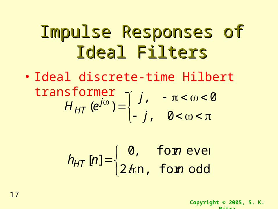
Impulse Responses of Ideal Impulse Responses of Ideal FiltersFilters
• Ideal discrete-time Hilbert transformer -
0,
0,)(
j
jeH j
HT
oddforn,2/
evenfor,0][
n
nnhHT

18Copyright © 2005, S. K. Mitra
Impulse Responses of Ideal Impulse Responses of Ideal FiltersFilters
• Ideal discrete-time differentiator -
0,)( jeH jDIF
0,cos0,0
][nn
nn
nhDIF

19
Digital Filter SpecificationsDigital Filter Specifications• As the impulse response corresponding to
each of these ideal filters is noncausal and of infinite length, these filters are not realizable
• In practice, the magnitude response specifications of a digital filter in the passband and in the stopband are given with some acceptable tolerances
• In addition, a transition band is specified between the passband and stopband

20
Digital Filter SpecificationsDigital Filter Specifications• For example, the magnitude response
of a digital lowpass filter may be given as indicated below
)( jeG

21
Digital Filter SpecificationsDigital Filter Specifications• As indicated in the figure, in the passband,
defined by , we require that with an error , i.e.,
• In the stopband, defined by , we require that with an error , i.e.,
1)( jeG
0)( jeG s
pp0
s
ppj
p eG ,1)(1
ss
jeG ,)(

22
Digital Filter SpecificationsDigital Filter Specifications• - passband edge frequency
• - stopband edge frequency
• - peak ripple value in the passband
• - peak ripple value in the stopband
• Since is a periodic function of , and of a real-coefficient digital filter is an even function of
• As a result, filter specifications are given only for the frequency range
p
s
sp
)( jeG)( jeG
0

23
Digital Filter SpecificationsDigital Filter Specifications
• Specifications are often given in terms of loss function A in dB
• Peak passband ripple
dB
• Minimum stopband attenuation
dB
)(log20)( 10 jeG
)1(log20 10 pp
)(log20 10 ss

26
Digital Filter SpecificationsDigital Filter Specifications
• For the normalized specification, maximum value of the gain function or the minimum value of the loss function is 0 dB
• Maximum passband attenuation -
dB
• For , it can be shown that
dB
210max 1log20
1 p
)21(log20 10max p

27
Digital Filter SpecificationsDigital Filter Specifications• In practice, passband edge frequency
and stopband edge frequency are specified in Hz
• For digital filter design, normalized bandedge frequencies need to be computed from specifications in Hz using
TFF
F
F pT
p
T
pp
2
2
TFFF
F sT
s
T
ss 2
2
sFpF

28
Digital Filter SpecificationsDigital Filter Specifications
• Example - Let kHz, kHz, and kHz
• Then
7pF 3sF25TF
56.01025
)107(23
3
p
24.01025
)103(23
3
s

29
• The transfer function H(z) meeting the frequency response specifications should be a causal transfer function
• For IIR digital filter design, the IIR transfer function is a real rational function of :
• H(z) must be a stable transfer function and must be of lowest order N for reduced computational complexity
Selection of Filter TypeSelection of Filter Type
1z
NMzdzdzdd
zpzpzppzH
NN
MM
,)(
22
110
22
110

30
Selection of Filter TypeSelection of Filter Type• For FIR digital filter design, the FIR
transfer function is a polynomial in with real coefficients:
• For reduced computational complexity, degree N of H(z) must be as small as possible
• If a linear phase is desired, the filter coefficients must satisfy the constraint:
N
n
nznhzH0
][)(
][][ nNhnh
1z

31
Selection of Filter TypeSelection of Filter Type• Advantages in using an FIR filter -
(1) Can be designed with exact linear phase,
(2) Filter structure always stable with quantized coefficients
• Disadvantages in using an FIR filter - Order of an FIR filter, in most cases, is considerably higher than the order of an equivalent IIR filter meeting the same specifications, and FIR filter has thus higher computational complexity

32
Digital Filter Design: Digital Filter Design: Basic ApproachesBasic Approaches
• Most common approach to IIR filter design - (1) Convert the digital filter specifications into an analog prototype lowpass filter specifications
• (2) Determine the analog lowpass filter transfer function
• (3) Transform into the desired digital transfer function
)(sHa
)(zG)(sHa

33
Digital Filter Design: Digital Filter Design: Basic ApproachesBasic Approaches
• This approach has been widely used for the following reasons:(1) Analog approximation techniques are highly advanced(2) They usually yield closed-form solutions(3) Extensive tables are available for analog filter design(4) Many applications require digital simulation of analog systems

34
Digital Filter Design: Digital Filter Design: Basic ApproachesBasic Approaches
• FIR filter design is based on a direct approximation of the specified magnitude response, with the often added requirement that the phase be linear
• The design of an FIR filter of order M may be accomplished by finding either the length-(N+1) impulse response samples or the (N+1) samples of its frequency response
][nh
)( jeH
35
Digital Filter Design: Digital Filter Design: Basic ApproachesBasic Approaches
• Three commonly used approaches to FIR filter design -
(1) Windowed Fourier series approach
(2) Frequency sampling approach
(3) Computer-based optimization methods

36Copyright © 2005, S. K. Mitra
Gibbs PhenomenonGibbs Phenomenon
• Gibbs phenomenon - Oscillatory behavior in the magnitude responses of causal FIR filters obtained by truncating the impulse response coefficients of ideal filters
0 0.2 0.4 0.6 0.8 10
0.5
1
1.5
/
Mag
nitu
de
N = 20N = 60

37Copyright © 2005, S. K. Mitra
Gibbs PhenomenonGibbs Phenomenon• As can be seen, as the length of the lowpass
filter is increased, the number of ripples in both passband and stopband increases, with a corresponding decrease in the ripple widths
• Height of the largest ripples remain the same independent of length
• Similar oscillatory behavior observed in the magnitude responses of the truncated versions of other types of ideal filters

38Copyright © 2005, S. K. Mitra
Gibbs PhenomenonGibbs Phenomenon• Gibbs phenomenon can be explained by
treating the truncation operation as an windowing operation:
• In the frequency domain
• where and are the DTFTs of and , respectively
][][][ nwnhnh dt
deeHeH jjd
jt )()()( )(
21
)( jt eH )( je
][nht ][nw
39Copyright © 2005, S. K. Mitra
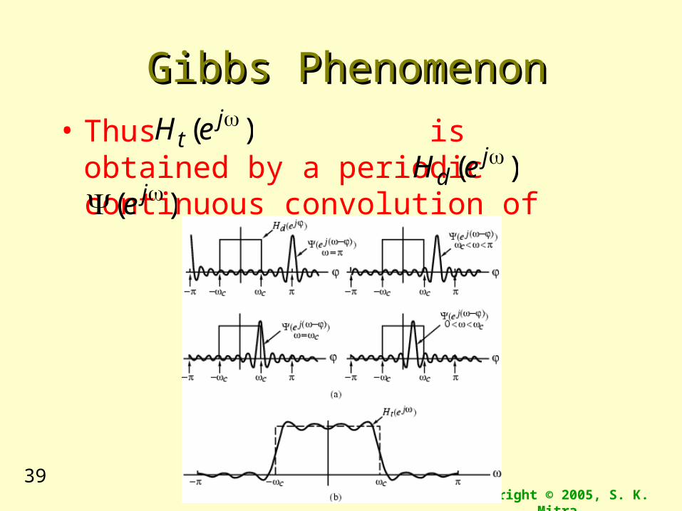
Gibbs PhenomenonGibbs Phenomenon• Thus is obtained by a periodic
continuous convolution of with)( j
t eH
)( je)( j
d eH
40Copyright © 2005, S. K. Mitra
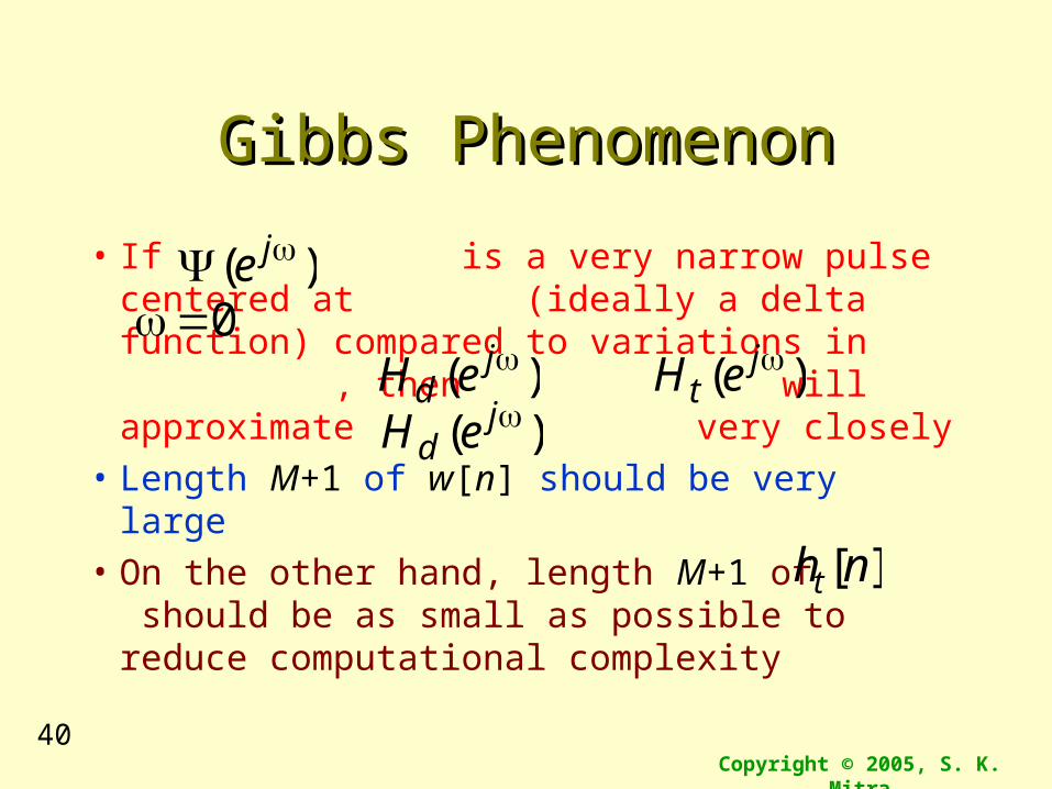
Gibbs PhenomenonGibbs Phenomenon
• If is a very narrow pulse centered at (ideally a delta function) compared
to variations in , then will approximate very closely
• Length M+1 of w[n] should be very large
• On the other hand, length M+1 of should be as small as possible to reduce computational complexity
)( je
)( jd eH
)( jd eH
)( jt eH
][nht
0

41Copyright © 2005, S. K. Mitra
Gibbs PhenomenonGibbs Phenomenon• A rectangular window is used to achieve
simple truncation:
• Presence of oscillatory behavior in is basically due to:– 1) is infinitely long and not absolutely
summable, and hence filter is unstable– 2) Rectangular window has an abrupt transition
to zero
otherwise,0
0,1][
MnnwR
)( jt eH
][nhd

42Copyright © 2005, S. K. Mitra
Gibbs PhenomenonGibbs Phenomenon• Oscillatory behavior can be explained by
examining the DTFT of :
• has a main lobe centered at
• Other ripples are called sidelobes
][nwR)( jR e
)( jR e 0
-1 -0.5 0 0.5 1-10
0
10
20
30
/
Am
plitu
deRectangular window
M = 4
M = 10 main lobe
side lobe

43Copyright © 2005, S. K. Mitra
Gibbs PhenomenonGibbs Phenomenon• Main lobe of characterized by its
width defined by first zero crossings on both sides of
• As M increases, width of main lobe decreases as desired
• Area under each lobe remains constant while width of each lobe decreases with an increase in M
• Ripples in around the point of discontinuity occur more closely but with no decrease in amplitude as M increases
)( jR e
0)1/(4 M
)( jt eH

44Copyright © 2005, S. K. Mitra
Gibbs PhenomenonGibbs Phenomenon• Rectangular window has an abrupt transition
to zero outside the range , which results in Gibbs phenomenon in
• Gibbs phenomenon can be reduced either:
(1) Using a window that tapers smoothly to zero at each end, or
(2) Providing a smooth transition from passband to stopband in the magnitude specifications
2/2/ MnM
)( jt eH

45Copyright © 2005, S. K. Mitra
Fixed Window FunctionsFixed Window Functions• Using a tapered window causes the height
of the sidelobes to diminish, with a corresponding increase in the main lobe width resulting in a wider transition at the discontinuity
• Hann:
• Hamming:
• Blackman:)4cos(08.0)2cos(5.042.0][ MnMnnw
),2cos(46.054.0][ Mnnw
),2cos(5.05.0][M
nnw 2/2/ MnM
2/2/ MnM
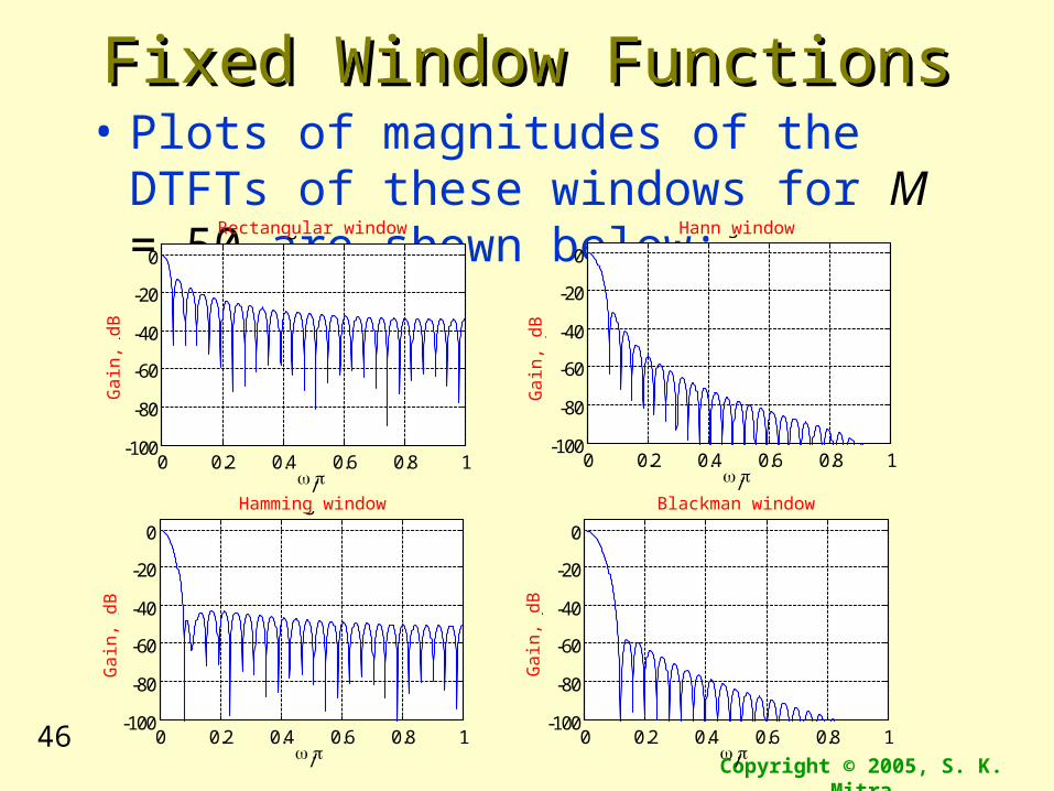
46Copyright © 2005, S. K. Mitra
Fixed Window FunctionsFixed Window Functions• Plots of magnitudes of the DTFTs of these
windows for M = 50 are shown below:
0 0.2 0.4 0.6 0.8 1-100
-80
-60
-40
-20
0
/
Gai
n, d
B
Rectangular window
0 0.2 0.4 0.6 0.8 1-100
-80
-60
-40
-20
0
/
Gai
n, d
B
Hanning window
0 0.2 0.4 0.6 0.8 1-100
-80
-60
-40
-20
0
/
Gai
n, d
B
Hamming window
0 0.2 0.4 0.6 0.8 1-100
-80
-60
-40
-20
0
/
Gai
n, d
B
Blackman window
Hann window
Gai
n, d
B
Gai
n, d
B
Gai
n, d
B
Gai
n, d
B
Rectangular window
Hamming window Blackman window

47Copyright © 2005, S. K. Mitra
Fixed Window FunctionsFixed Window Functions
• Magnitude spectrum of each window characterized by a main lobe centered at = 0 followed by a series of sidelobes with decreasing amplitudes
• Parameters predicting the performance of a window in filter design are:
• Main lobe width
• Relative sidelobe level

48Copyright © 2005, S. K. Mitra
Fixed Window FunctionsFixed Window Functions
• Main lobe width - given by the distance between zero crossings on both sides of main lobe
• Relative sidelobe level - given by the difference in dB between amplitudes of largest sidelobe and main lobe
ML
sA

49Copyright © 2005, S. K. Mitra
Fixed Window FunctionsFixed Window Functions
• Observe
• Thus,
• Passband and stopband ripples are the same
1)()( )()( cc jt
jt eHeH
5.0)( cjt eH

50Copyright © 2005, S. K. Mitra
Fixed Window FunctionsFixed Window Functions
• Distance between the locations of the maximum passband deviation and minimum stopband value
• Width of transition band
ML
MLps

51Copyright © 2005, S. K. Mitra
Fixed Window FunctionsFixed Window Functions
• To ensure a fast transition from passband to stopband, window should have a very small main lobe width
• To reduce the passband and stopband ripple , the area under the sidelobes should be very small
• Unfortunately, these two requirements are contradictory

52Copyright © 2005, S. K. Mitra
Fixed Window FunctionsFixed Window Functions
• In the case of rectangular, Hann, Hamming, and Blackman windows, the value of ripple does not depend on filter length or cutoff frequency , and is essentially constant
• In addition,
where c is a constant for most practical purposes
Mc
c

53Copyright © 2005, S. K. Mitra
Fixed Window FunctionsFixed Window Functions• Rectangular window -
dB, dB,
• Hann window -
dB, dB,
• Hamming window -
dB, dB,
• Blackman window -
dB, dB,
)1/(4 MML
)1/(8 MML
)1/(8 MML
)1/(12 MML
3.13sA
5.31sA
7.42sA
1.58sA
9.20s
9.43s
5.54s
3.75s
)2//(92.0 M
)2//(11.3 M
)2//(32.3 M
)2//(56.5 M

54Copyright © 2005, S. K. Mitra
Fixed Window FunctionsFixed Window Functions• Filter Design Steps -
(1) Set
(2) Choose window based on specified
(3) Estimate M using
(4) Find coefficients by multiplying ideal impulse response with the window function
(5) Shift by M/2 samples to make the filter causalMc
2/)( spc
s

55Copyright © 2005, S. K. Mitra
FIR Filter Design ExampleFIR Filter Design Example• Lowpass filter of length 51 and 2/c
0 0.2 0.4 0.6 0.8 1
-100
-50
0
/
Gai
n, d
B
Lowpass Filter Designed Using Blackman window
0 0.2 0.4 0.6 0.8 1
-100
-50
0
/
Gai
n, d
B
Lowpass Filter Designed Using Hann window
0 0.2 0.4 0.6 0.8 1
-100
-50
0
/
Gai
n, d
B
Lowpass Filter Designed Using Hamming window

56Copyright © 2005, S. K. Mitra
Adjustable Window FunctionsAdjustable Window Functions• Kaiser Window -
where is an adjustable parameter and is the modified zeroth-order Bessel function of the first kind:
• Note for u > 0
• In practice
2/2/,)(
})/2(1{][
0
20 MnM
I
MnInw
1
20 ]
!)2/([1)(
r
r
ruuI
0)(0 uI
20
1
20 ]
!)2/([1)(
r
r
ruuI
)(0 uI

57Copyright © 2005, S. K. Mitra
Adjustable Window FunctionsAdjustable Window Functions• controls the minimum stopband
attenuation of the windowed filter response• is estimated using
• Filter order is estimated using
where is the normalized transition bandwidth
,0
),21(07886.04.0)21(5842.0
),7.8(1102.0
ss
s
21for
5021for
50for
s
s
s
)(285.2
8
sM

58Copyright © 2005, S. K. Mitra
FIR Filter Design ExampleFIR Filter Design Example• Specifications: , ,
dB
• Thus
• Choose M = 24
01.010 20/ ss
40s
3.0p 5.0s
4.02/)( spc
3953.31907886.0)19(5842.0 4.0
2886.22)2.0(285.2
32
M