1

Fault Dynamics of theApril 6, 2009 L'Aquila, Italy

Earthquake Sequence

Robert B. HerrmannSaint Louis University

Luca MalagniniINGV, Roma

2

Overview• Determined moment tensor solutions

for 102 of 160 earthquakes with ML ≥ 3

• Developed regional crustal model that fits ground velocities well in the 0.02 – 0.20 Hz frequency band

• Evaluated INGV ML and source depth

• Noted stations that are difficult to fit• Make recommendations on digital

network

3

Moment Tensor Solution

• Initially used WUS model• Developed regional velocity model

from–DSS study– Love and Rayleigh wave dispersion from

L'Aquila aftershocks–Receiver functions

4

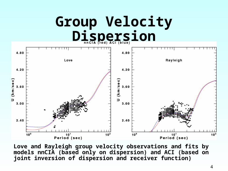
Group Velocity Dispersion

Love and Rayleigh group velocity observations and fits by models nnCIA (based only on dispersion) and ACI (based on joint inversion of dispersion and receiver function)

5

Receiver function fits at AQU using ACI model

• Used iterative deconvolution

• Used filter α = 0.5 and 1.0

• Reverberations due to surface low-velocity and crustal velocity inversions

6

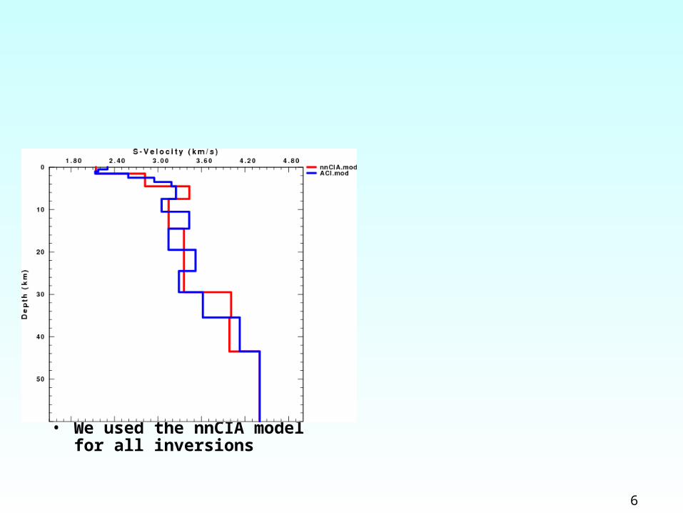
• Group velocities require low velocities near the surface.

• Receiver functions provide more detail on crust.

• Both models fit waveforms very well in the 0.02 – 0.20 Hz band in for the 0 – 150 km epicentral distance range.

• At these frequencies, discontinuities are averaged

• We used the nnCIA model for all inversions

7

Waveform fitsComparison of observed and model predicted waveforms for earthquake of 20090423151408

STK=345, DIP-30RAKE=-50, MW=3.84

•Each trace pair is plotted to the same scale: observed is red, blue is predicted

•All traces represent filtered velocity in the 0.02 – 0.10 Hz band

•Waveform shapes are excellent

•Some stations have problems and were not used for moment tensor

8

Moment Tensor Solutions

• M < 3 (black for seismicity – no inversion)

• 3 < M < 4 (blue)

• 4 < M < 5 (blue-green)

• 5 < M < 5.5 (yellow)

• 5.5 < M (red) (IDIDE locations and magnitudes)

9

Moment Tensorscolored by depth

• Main Mw=6.25 plotted at INGV epicenter not at centroid

• Northern group shows a pattern of down-dip to SE

• Southern group also shows same pattern

10

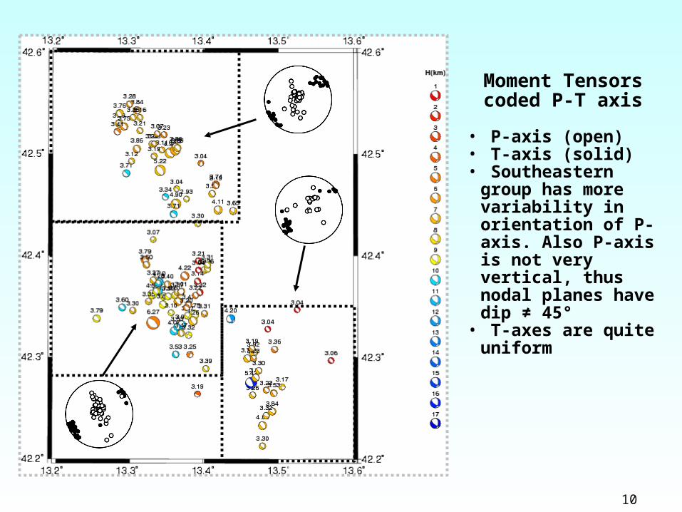
Moment Tensorscoded P-T axis

• P-axis (open)• T-axis (solid)• Southeastern group

has more variability in orientation of P- axis. Also P-axis is not very vertical, thus nodal planes have dip ≠ 45°

• T-axes are quite uniform

11

Comparison of Moment Tensor and INGV Depths and Magnitudes

Comparison of Depths Comparison of magnitudes

12

Source Complexity• We were able to get the moment

tensor solution for the main event by using the frequency band 0.01 – 0.025 Hz

• This was strange since we used 0.01 – 0.05 Hz for the Mw=5.91 2008/02/21 Wells, Nevada earthquake

• Using a 0.01 – 0.05 band gave an unrealistic depth of 29 km for L'Aquila

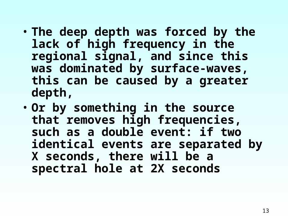
13

• The deep depth was forced by the lack of high frequency in the regional signal, and since this was dominated by surface-waves, this can be caused by a greater depth,

• Or by something in the source that removes high frequencies, such as a double event: if two identical events are separated by X seconds, there will be a spectral hole at 2X seconds

14

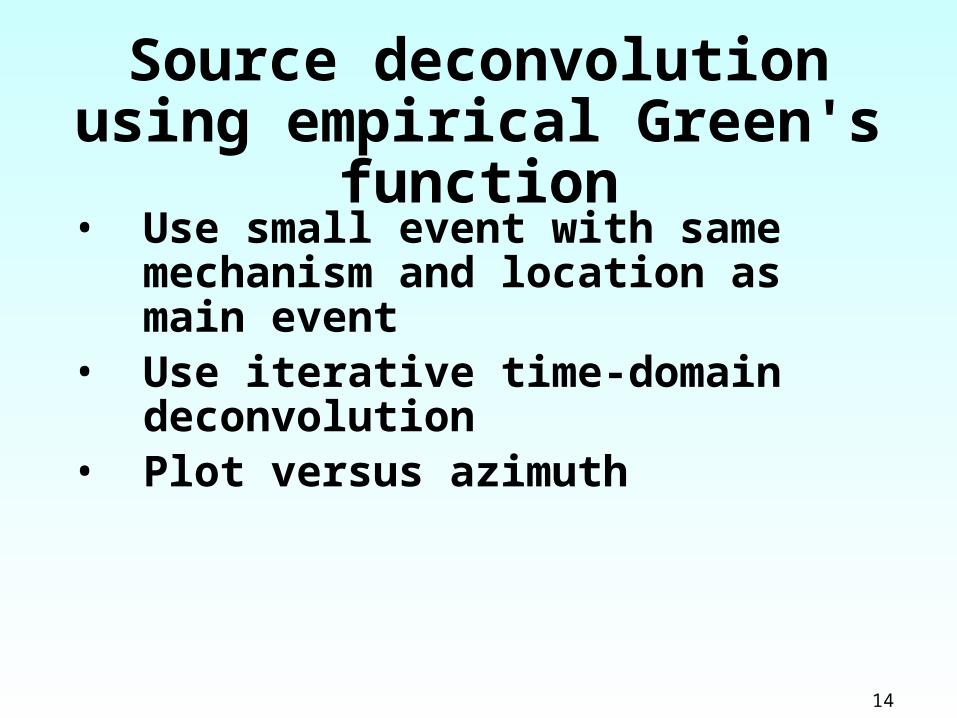
Source deconvolution using empirical Green's function

• Use small event with same mechanism and location as main event

• Use iterative time-domain deconvolution

• Plot versus azimuth

15

Comparison

• Wells, Nevada– 20080221141605 (Mw = 5.88)– 20080228151039 (Mw = 3.98)

16

Comparison

• Laquila– 20090406013239 (Mw = 6.25)– 20090406035645 (Mw = 4.26)

17

Wells

18

L'Aquila

19

• L'Aquila earthquake is more complex than Wells

• Azimuthal coverage is not very good though

• Speculation – is source complexity reason for low ML?

20

Network Performance

• Excellent data through ISIDe• World class broadband network• Data drops–No problem for moment tensor inversion

because there are many other good stations

• Station responses–Never used CAMP since gains seem to

be afactor of 2-3 too large–Never used TRTR because of gain and

waveform shape – local site effect?

21

– VVLD low frequency sensor noise/instability

–CERT – station gain too low?– LNSS – low frequency noise–RNI2 ?

To process the moment tensors rapidly, we did not keep a complete list of problem stations. CAMP was often the nearest station and would have been very useful for smaller earthquakes

22

Observations

• Moment tensors can be done in near-real time by an analyst. All codes and Green's functions are set up and easy to use.

• The main event seems may be a multiple source. The lack of on-scale data at distances < 50 km, and for many < 100, makes study of main event difficult

23

• Rapid finite fault inversion may be useful for estimating where significant aftershocks may occur. –Most moment tensor solutions are on

edge of region of the initial rupture.

• Real-time finite fault inversion requires on-scale data. Perhaps install continuous low-gain seismic channels (e.g., Episensor) at all or every second or third broadband station.

24

Summary

• We compiled a very complete catalog of moment tensors down to M=3

• The pre-computed Green's functions can be used for other earthquakes in the country