1

Energy-Efficient Clustering/Routing for

Cooperative MIMO Operation in Sensor Networks

Mohammad Z. Siam and Marwan Krunz Ossama Younis

Department of Electrical and Computer Engineering Applied Research, Telcordia Technologies, Inc.

University of Arizona, Tucson, AZ 85721 Piscataway, NJ 08854

{siam, krunz}@ece.arizona.edu oyounis@research.telcordia.com

Technical Report

TR-UA-ECE-2008-2

August 2008

Abstract

Employing multi-input multi-output (MIMO) links can improve energy efficiency in wireless sensor networks (WSNs).

Although a sensor node is likely to be equipped with only one antenna, it is possible to group several sensors to form a virtual

MIMO link. Such grouping can be formed by means of clustering. In this paper, we propose a distributed MIMO-adaptive

energy-efficient clustering/routing scheme, coined cooperative MIMO (CMIMO), which aims at reducing energy consumption

in multi-hop WSNs. In CMIMO, each cluster has two cluster heads (CHs), which are responsible for routing traffic between

clusters (i.e., inter-cluster communications). CMIMO has the ability to adapt the transmission mode and transmission power

on a per-packet basis. The transmission mode can be one of four transmit/receive configurations: 1× 1 (SISO), 2× 1 (MISO),

1× 2 (SIMO), and 2× 2 (MIMO). We study the performance of CMIMO via simulations. Results indicate that our proposed

scheme achieves a significant reduction in energy consumption, compared to non-adaptive clustered WSNs.

Index Terms

Sensor networks, clustering, routing, MIMO, diversity gain, energy efficiency.

2

I. INTRODUCTION

Nodes in wireless sensor networks (WSNs) are typically powered by small batteries. Replacement or recharging of these

sensors is typically difficult due to two reasons: (1) sensors are deployed in large numbers, making the process of collecting

them back for recharging expensive and time consuming, and (2) in some environments, such as disaster areas, it can

be infeasible to reach the sensors once they are deployed. Consequently, improving the energy efficiency in WSNs has

always been a primary objective in recent research. Several approaches have been proposed to achieve this objective. One

approach is to control the transmission power (e.g., [1]). Another approach is to cluster the nodes to reduce the number of

communications across the network (e.g., [2]). A third approach is to put some nodes to sleep according to their duty cycles

(e.g., [3]). A recently advocated approach to achieve energy efficiency is to exploit the proximity between nodes and let

them operate as a multi-input multi-output (MIMO) system (e.g., [4], [5], [6]). In this work, we focus on the last approach.

MIMO technology has the potential to increase channel capacity and reduce transmission energy consumption in fading

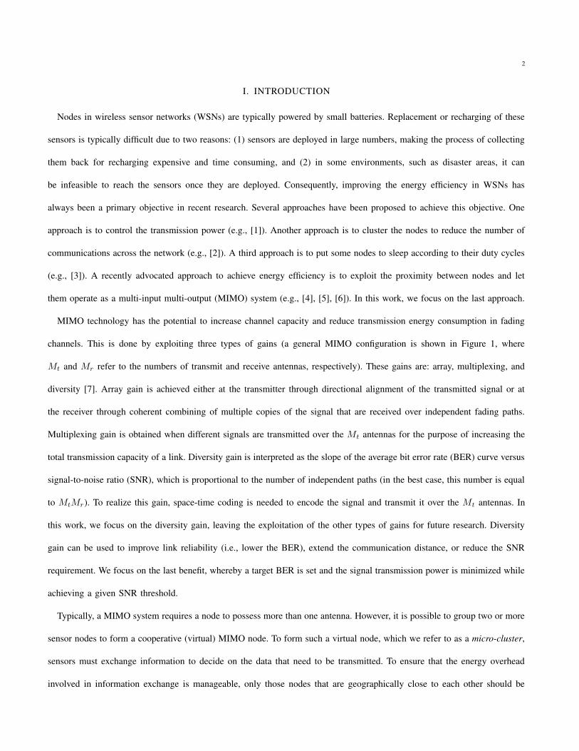
channels. This is done by exploiting three types of gains (a general MIMO configuration is shown in Figure 1, where

Mt and Mr refer to the numbers of transmit and receive antennas, respectively). These gains are: array, multiplexing, and

diversity [7]. Array gain is achieved either at the transmitter through directional alignment of the transmitted signal or at

the receiver through coherent combining of multiple copies of the signal that are received over independent fading paths.

Multiplexing gain is obtained when different signals are transmitted over the Mt antennas for the purpose of increasing the

total transmission capacity of a link. Diversity gain is interpreted as the slope of the average bit error rate (BER) curve versus

signal-to-noise ratio (SNR), which is proportional to the number of independent paths (in the best case, this number is equal

to MtMr). To realize this gain, space-time coding is needed to encode the signal and transmit it over the Mt antennas. In

this work, we focus on the diversity gain, leaving the exploitation of the other types of gains for future research. Diversity

gain can be used to improve link reliability (i.e., lower the BER), extend the communication distance, or reduce the SNR

requirement. We focus on the last benefit, whereby a target BER is set and the signal transmission power is minimized while

achieving a given SNR threshold.

Typically, a MIMO system requires a node to possess more than one antenna. However, it is possible to group two or more

sensor nodes to form a cooperative (virtual) MIMO node. To form such a virtual node, which we refer to as a micro-cluster,

sensors must exchange information to decide on the data that need to be transmitted. To ensure that the energy overhead

involved in information exchange is manageable, only those nodes that are geographically close to each other should be

3

1

M t

1

M r

Transmitter side Receiver side

2

3

2

3

Fig. 1. MIMO configuration.

grouped to form a cooperative MIMO node. Most proposed cooperative MIMO systems have not considered multi-hop

communications, and focused only on single-hop communications. Multi-hop communications are essential for large-scale

networks that contain sensors with limited transmission ranges.

MIMO systems also need to perform early data aggregation to reduce redundancy and save energy. Data redundancy

is created by relaying the signal to closeby users, which act as intermediate transmitters. Cooperative MIMO for WSNs

distinguishes itself in terms of data redundancy from user cooperative MIMO systems that were proposed in [8], [9], and [10].

In a WSN, the sensed data from neighboring nodes intrinsically presents rich redundancy because of the high correlation of

spatial events that occur within a certain locality. Cooperative MIMO techniques are designed to eliminate data redundancy

by aggregating data as early as possible, prior to forwarding it. Data aggregation is done by exploiting node clustering, which

organizes the network into a connected hierarchy. In the context of WSNs, clustering involves grouping nodes and electing a

cluster head (CH) such that the non-CH nodes of a cluster can communicate with their CH directly. CHs forward aggregated

data to the sink directly or via other CHs. Thus, the collection of CHs in the network forms a connected dominating set.

In this paper, we propose a distributed MIMO-adaptive energy-efficient clustering/routing scheme, coined cooperative

MIMO (CMIMO), for multi-hop WSNs. In this scheme, each cluster has two CHs, which are responsible for inter-cluster

communications. Clustering is done based on the remaining energy of nodes, neighbor proximity, and the size of neighbor

lists. The rationale for selecting these criteria is to build cooperative MIMO links whose effect is as close as possible to

actual MIMO systems (with two antennas per node) and that have manageable overhead. Diversity gain of such a cooperative

MIMO node is maximized by adapting the “transmission mode” and the transmission power of inter-cluster communications

on a per-packet basis. By “transmission mode” we mean one of four transmit/receive configurations: 1 × 1 (single-input

4

single-output / SISO), 2 × 1 (multi-input single-output / MISO), 1 × 2 (single-input multi-output / SIMO), and 2 × 2

(multi-input multi-output / MIMO)1. The total energy consumption that our scheme minimizes consists of transmission and

circuit energies. For a given target BER, a multi-antenna transmission requires less transmission power than a SISO system.

However, it also requires more circuit power at both ends of the link. As a result, a distance-dependent tradeoff emerges

between transmission and circuit powers [12]: For relatively small distances, circuit power is dominant, and hence a SISO

mode is more energy-efficient than a multi-antenna mode. As the transmitter-receiver distance increases, the tradeoff shifts

in favor of multi-antenna modes (SIMO, MISO, MIMO).

The rest of the paper is organized as follows. We describe the CMIMO scheme in section II. The system model along with

the overall energy consumption of CMIMO are analyzed in section III. In section IV we discuss some issues related to the

design of CMIMO, including connectivity, listening cost, synchronization, reclustering, and medium access control (MAC).

The performance of the proposed scheme is evaluated via simulations in section V. Section VI describes related work.

Section VII discusses the main conclusions of this paper as well as some generalizations and extensions of the proposed

CMIMO scheme.

II. THE CMIMO SCHEME

In this section, we first give an overview of the proposed CMIMO scheme, followed by more operational details.

A. Overview

CMIMO is a distributed MIMO-adaptive energy-efficient scheme that aims at minimizing the total energy consumption

(transmission plus circuit energies) in multi-hop WSNs. It employs a dynamic clustering approach with up to two CHs

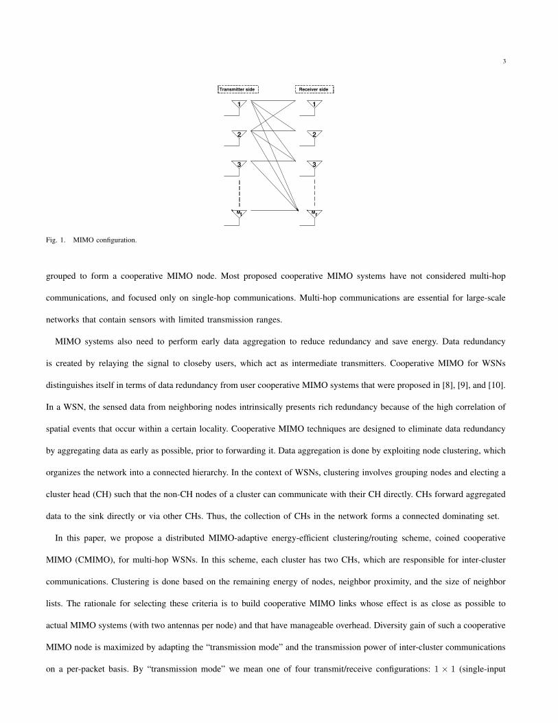
per cluster: a master CH (MCH) and a slave CH (SCH). The two CHs operate as a cooperative MIMO node for inter-

cluster communications (see Figure 2). The operation of CMIMO has three main phases: cluster formation, intra-cluster

communications, and inter-cluster communications with cooperative MIMO capabilities. We discuss these phases in detail

in the following subsection. Cluster formation is done in a distributed way, and results in at most two CHs per cluster (the

MCH is mandatory whereas the SCH may or may not be present). During intra-cluster communications, the selected MCH

is responsible for aggregating data sent by other nodes in the cluster and exchanging this data with the SCH, so that the

two CHs operate as a cooperative MIMO node (if needed). When data is available at the CHs of the source micro-cluster,

1The feasibility of adapting the transmission mode on a per-packet basis was demonstrated in several experimental MIMO platforms [11].

5

inter-cluster communications are carried out by forwarding/exchanging data with other micro-clusters or directly with the

sink. An energy-efficient routing algorithm is executed over the topology of virtual MIMO nodes to determine the end-to-end

path that minimizes the total energy consumption among all possible paths between the CHs and the sink. The MCH (or both

MCH and SCH) of the receiving cluster selects the optimal transmission mode and transmission power for communication

with other CHs. The mode and power can be different for different hops, depending on the distances between CHs in

different clusters.

MCH

SCH

MCH

SCH MCH

SCH

MCH

SCH

SCH

MCH

MCH MCH SCH

SCH

MCH

MCH MCH

MCH MCH SCH SCH

MCH MCH MCH

SCH SCH SCH

MCH

…

... ...

...

...

. . . . . .

. . .

. . .

. . .

MIMO link

MISO link

Micro cluster

Micro cluster

Sink

SIMO link

SISO link

MCH/SCH node non-MCH/SCH node

Fig. 2. Example topology of a clustered WSN with cooperative MIMO.

Our design is applicable to micro-clusters with more than two CHs. To simplify the exposition, we limit the number of

CHs per cluster in this work to two. Note, however, that a higher number of CHs may result in more energy overhead,

especially for intra-cluster communications. Therefore, we cannot assert that having more CHs in a micro-cluster improves

the overall performance, compared to that of a 2 × 2 MIMO system.

Before delving into the operational details of CMIMO, we note that using cooperative MIMO systems results in additional

overhead than usual MIMO systems, due to the need for the two CHs in a micro-cluster to exchange information, and also the

CHs of two adjacent micro-clusters. However, the overall gain behind cooperative-MIMO systems is still prevalent compared

to non-adaptive clustering systems, especially when large distances exist between different clusters. This is demonstrated in

6

our simulations in section V.

B. Operational Details

In this section, we describe the operational details of the CMIMO scheme, including cluster formation, intra-cluster

communications, and inter-cluster communications with cooperative MIMO capabilities.

1) Cluster formation: The cluster formation process consists of the following steps:

Step 1: Neighborhood discovery: In this step, each node in the network uses the classic carrier sense multiple access

with collision avoidance (CSMA/CA) scheme to contend for the wireless channel. Once a node v succeeds in accessing

the channel, it sends a “hello” message at a fixed transmission power (Pintra) to discover its 1-hop neighbors. This hello

message carries the following information: node ID, its remaining energy, and a list of v’s neighbors (nodes that v has

received hello messages from). What triggers node v to send a hello message is one of the following two factors. First, if

v receives a hello message from a node, say u, that is not included in v’s neighbor list, v adds u to its neighbor list and

broadcasts the updated list to its neighbors. Second, if v receives a hello message from an already known neighbor u and the

neighbor list of u does not include v, v broadcasts a hello message to inform u about itself. In general, a node sends hello

messages as soon as it joins the network and whenever it hears from new neighbors. Therefore, the algorithm is progressive,

i.e., the hello messages contain updated neighbors list in each subsequent broadcast.

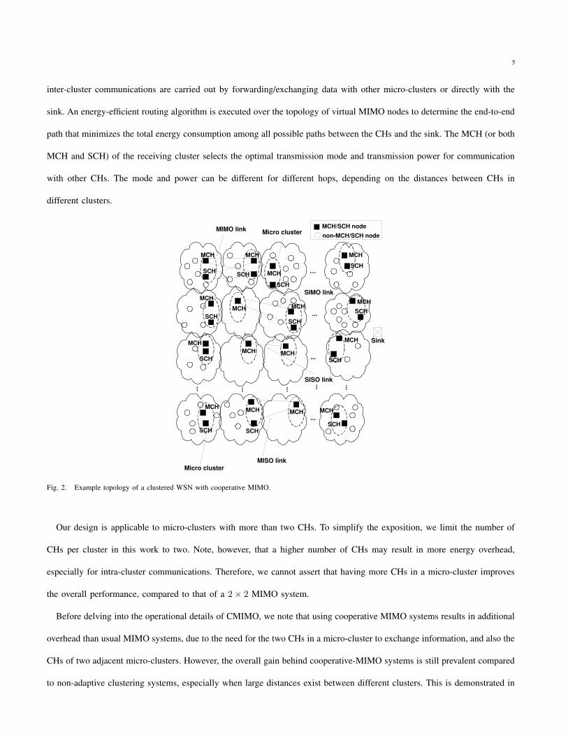
We now explain the neighborhood discovery process through an example. Consider the network in Figure 3. The first

number at each node indicates the node ID, whereas the second number indicates the remaining energy of that node. Dashed

lines between any two nodes in this figure show that these nodes are neighbors, i.e., they can directly communicate with each

other (this information is initially unknown to the nodes). Assume that according to the CSMA/CA scheme, the sequence of

transmissions is as follows: nodes 1 and 5 send first (they are not neighbors, i.e., they cannot hear each other), followed by

node 2, then node 4, and finally node 3. Node 1 sends its hello message, informing others about its ID (N1), its remaining

energy (E1), and that it has not heard from any neighbors yet. Node 5 sends its hello message, including its ID (N5),

its remaining energy (E5), and its neighbors list, which is still empty. Node 2 sends its hello message, which contains its

ID (N2), its remaining energy (E2), and its neighbors list, which has one neighbor (N1). Node 4 sends its hello message,

informing the other nodes about its ID (N4), its remaining energy (E4), and its neighbors list, which has three neighbors

(nodes 1, 2, and 5). Finally, node 3 sends a hello message that includes its ID (N3), its remaining energy (E3), and its

neighbors list. Suppose that the hello messages from N1 and N5 collided at node 3, so node 3 is aware of only two neighbors

7

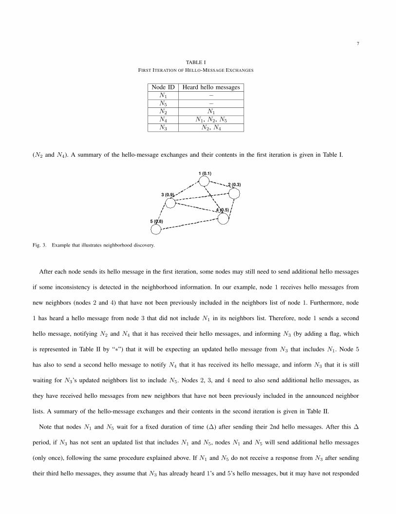
TABLE IFIRST ITERATION OF HELLO-MESSAGE EXCHANGES

Node ID Heard hello messagesN1 −N5 −N2 N1

N4 N1, N2, N5

N3 N2, N4

(N2 and N4). A summary of the hello-message exchanges and their contents in the first iteration is given in Table I.

5 (0.8)

3 (0.9)

4 (0.5)

2 (0.3)

1 (0.1)

Fig. 3. Example that illustrates neighborhood discovery.

After each node sends its hello message in the first iteration, some nodes may still need to send additional hello messages

if some inconsistency is detected in the neighborhood information. In our example, node 1 receives hello messages from

new neighbors (nodes 2 and 4) that have not been previously included in the neighbors list of node 1. Furthermore, node

1 has heard a hello message from node 3 that did not include N1 in its neighbors list. Therefore, node 1 sends a second

hello message, notifying N2 and N4 that it has received their hello messages, and informing N3 (by adding a flag, which

is represented in Table II by “∗”) that it will be expecting an updated hello message from N3 that includes N1. Node 5

has also to send a second hello message to notify N4 that it has received its hello message, and inform N3 that it is still

waiting for N3’s updated neighbors list to include N5. Nodes 2, 3, and 4 need to also send additional hello messages, as

they have received hello messages from new neighbors that have not been previously included in the announced neighbor

lists. A summary of the hello-message exchanges and their contents in the second iteration is given in Table II.

Note that nodes N1 and N5 wait for a fixed duration of time (∆) after sending their 2nd hello messages. After this ∆

period, if N3 has not sent an updated list that includes N1 and N5, nodes N1 and N5 will send additional hello messages

(only once), following the same procedure explained above. If N1 and N5 do not receive a response from N3 after sending

their third hello messages, they assume that N3 has already heard 1’s and 5’s hello messages, but it may have not responded

8

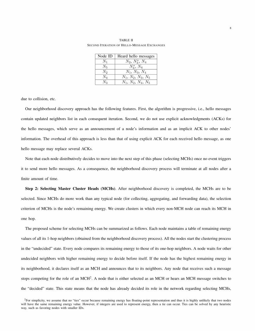
TABLE IISECOND ITERATION OF HELLO-MESSAGE EXCHANGES

Node ID Heard hello messagesN1 N2, N∗

3, N4

N5 N∗3

, N4

N2 N1, N3, N4

N4 N1, N2, N3, N5

N3 N1, N2, N4, N5

due to collision, etc.

Our neighborhood discovery approach has the following features. First, the algorithm is progressive, i.e., hello messages

contain updated neighbors list in each consequent iteration. Second, we do not use explicit acknowledgments (ACKs) for

the hello messages, which serve as an announcement of a node’s information and as an implicit ACK to other nodes’

information. The overhead of this approach is less than that of using explicit ACK for each received hello message, as one

hello message may replace several ACKs.

Note that each node distributively decides to move into the next step of this phase (selecting MCHs) once no event triggers

it to send more hello messages. As a consequence, the neighborhood discovery process will terminate at all nodes after a

finite amount of time.

Step 2: Selecting Master Cluster Heads (MCHs). After neighborhood discovery is completed, the MCHs are to be

selected. Since MCHs do more work than any typical node (for collecting, aggregating, and forwarding data), the selection

criterion of MCHs is the node’s remaining energy. We create clusters in which every non-MCH node can reach its MCH in

one hop.

The proposed scheme for selecting MCHs can be summarized as follows. Each node maintains a table of remaining energy

values of all its 1-hop neighbors (obtained from the neighborhood discovery process). All the nodes start the clustering process

in the “undecided” state. Every node compares its remaining energy to those of its one-hop neighbors. A node waits for other

undecided neighbors with higher remaining energy to decide before itself. If the node has the highest remaining energy in

its neighborhood, it declares itself as an MCH and announces that to its neighbors. Any node that receives such a message

stops competing for the role of an MCH2. A node that is either selected as an MCH or hears an MCH message switches to

the “decided” state. This state means that the node has already decided its role in the network regarding selecting MCHs,

2For simplicity, we assume that no “ties” occur because remaining energy has floating-point representation and thus it is highly unlikely that two nodeswill have the same remaining energy value. However, if integers are used to represent energy, then a tie can occur. Ties can be solved by any heuristicway, such as favoring nodes with smaller IDs.

9

i.e., it is either an MCH or cannot be an MCH because it has heard an MCH message. The remaining undecided nodes

repeat the above process until all the nodes are “decided.”

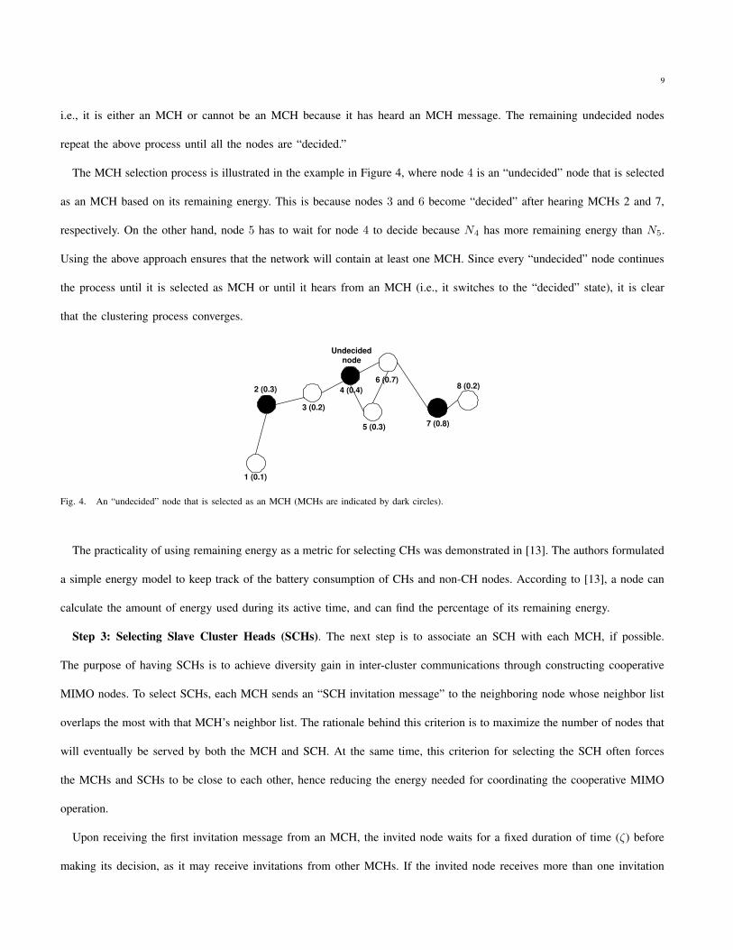
The MCH selection process is illustrated in the example in Figure 4, where node 4 is an “undecided” node that is selected

as an MCH based on its remaining energy. This is because nodes 3 and 6 become “decided” after hearing MCHs 2 and 7,

respectively. On the other hand, node 5 has to wait for node 4 to decide because N4 has more remaining energy than N5.

Using the above approach ensures that the network will contain at least one MCH. Since every “undecided” node continues

the process until it is selected as MCH or until it hears from an MCH (i.e., it switches to the “decided” state), it is clear

that the clustering process converges.

1 (0.1)

2 (0.3)

3 (0.2)

7 (0.8)

8 (0.2) 4 (0.4)

Undecided node

5 (0.3)

6 (0.7)

Fig. 4. An “undecided” node that is selected as an MCH (MCHs are indicated by dark circles).

The practicality of using remaining energy as a metric for selecting CHs was demonstrated in [13]. The authors formulated

a simple energy model to keep track of the battery consumption of CHs and non-CH nodes. According to [13], a node can

calculate the amount of energy used during its active time, and can find the percentage of its remaining energy.

Step 3: Selecting Slave Cluster Heads (SCHs). The next step is to associate an SCH with each MCH, if possible.

The purpose of having SCHs is to achieve diversity gain in inter-cluster communications through constructing cooperative

MIMO nodes. To select SCHs, each MCH sends an “SCH invitation message” to the neighboring node whose neighbor list

overlaps the most with that MCH’s neighbor list. The rationale behind this criterion is to maximize the number of nodes that

will eventually be served by both the MCH and SCH. At the same time, this criterion for selecting the SCH often forces

the MCHs and SCHs to be close to each other, hence reducing the energy needed for coordinating the cooperative MIMO

operation.

Upon receiving the first invitation message from an MCH, the invited node waits for a fixed duration of time (ζ) before

making its decision, as it may receive invitations from other MCHs. If the invited node receives more than one invitation

10

within ζ, it chooses the closest inviting MCH (based on the strength of the received signal). The invited node announces

its decision via an “SCH acceptance message,” enabling decided MCHs to look for other SCHs. Upon receiving an “SCH

acceptance message,” the intended MCH confirms this association via an “SCH confirmation message.” The purpose of this

message is to inform non-MCH neighbors of this MCH that they should not expect subsequent “SCH invitation messages”

from that MCH, so that they can move into the next step (cluster membership). The “SCH confirmation message” is sent at

a fixed power level (Pinter) that achieves network connectivity (we explain later how CMIMO results in a connected graph).

This Pinter ensures that the “SCH confirmation message” reaches at least the closest MCH to the sending MCH node. This

message plays a significant role in MCH-neighborhood discovery. Therefore, it includes the following fields: MCH ID, its

SCH ID, and a list of MCHs that the MCH has already received SCH confirmation messages from. The other steps of this

discovery approach are the same as in the neighborhood discovery explained previously.

Note that the MCH neighbors of the invited SCH should be able to receive the “SCH acceptance message.” Accordingly,

they will expect an upcoming “SCH confirmation message” from the inviting MCH to the invited SCH. As a consequence,

these MCHs defer from transmission during the “SCH confirmation message,” so as to avoid collisions at the SCH. Once

that message is transmitted, those MCHs start looking for other SCHs following the same approach explained above.

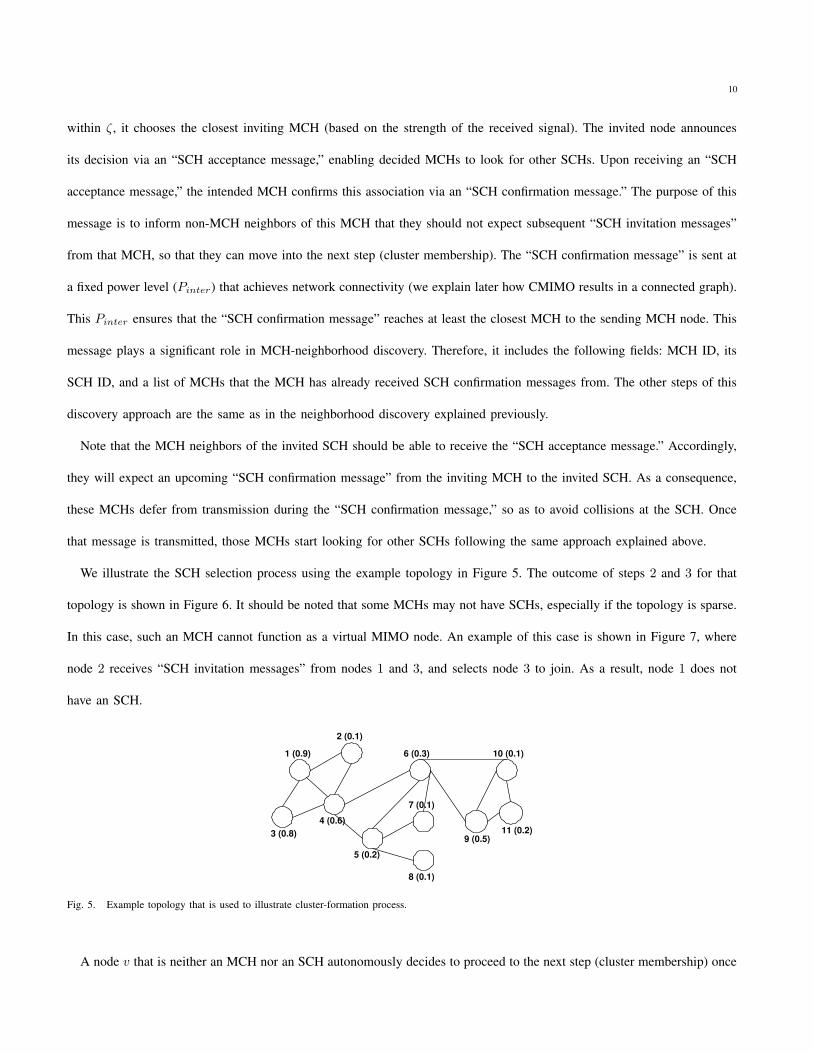
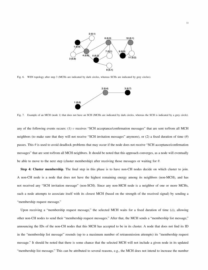
We illustrate the SCH selection process using the example topology in Figure 5. The outcome of steps 2 and 3 for that

topology is shown in Figure 6. It should be noted that some MCHs may not have SCHs, especially if the topology is sparse.

In this case, such an MCH cannot function as a virtual MIMO node. An example of this case is shown in Figure 7, where

node 2 receives “SCH invitation messages” from nodes 1 and 3, and selects node 3 to join. As a result, node 1 does not

have an SCH.

3 (0.8)

1 (0.9)

2 (0.1)

4 (0.6)

6 (0.3)

5 (0.2)

8 (0.1)

7 (0.1)

9 (0.5)

10 (0.1)

11 (0.2)

Fig. 5. Example topology that is used to illustrate cluster-formation process.

A node v that is neither an MCH nor an SCH autonomously decides to proceed to the next step (cluster membership) once

11

3 (0.8)

1 (0.9)

2 (0.1)

4 (0.6)

6 (0.3)

7 (0.1)

5 (0.2)

8 (0.1)

9 (0.5)

11 (0.2)

10 (0.1)

Fig. 6. WSN topology after step 3 (MCHs are indicated by dark circles, whereas SCHs are indicated by grey circles).

1 (0.6)

2 (0.4) 3 (0.7)

Fig. 7. Example of an MCH (node 1) that does not have an SCH (MCHs are indicated by dark circles, whereas the SCH is indicated by a grey circle).

any of the following events occurs: (1) v receives “SCH acceptance/confirmation messages” that are sent to/from all MCH

neighbors (to make sure that they will not receive “SCH invitation messages” anymore), or (2) a fixed duration of time (θ)

passes. This θ is used to avoid deadlock problems that may occur if the node does not receive “SCH acceptance/confirmation

messages” that are sent to/from all MCH neighbors. It should be noted that this approach converges, as a node will eventually

be able to move to the next step (cluster membership) after receiving those messages or waiting for θ.

Step 4: Cluster membership. The final step in this phase is to have non-CH nodes decide on which cluster to join.

A non-CH node is a node that does not have the highest remaining energy among its neighbors (non-MCH), and has

not received any “SCH invitation message” (non-SCH). Since any non-MCH node is a neighbor of one or more MCHs,

such a node attempts to associate itself with its closest MCH (based on the strength of the received signal) by sending a

“membership request message.”

Upon receiving a “membership request message,” the selected MCH waits for a fixed duration of time (φ), allowing

other non-CH nodes to send their “membership request messages.” After that, the MCH sends a “membership list message,”

announcing the IDs of the non-CH nodes that this MCH has accepted to be in its cluster. A node that does not find its ID

in the “membership list message” resends (up to a maximum number of retransmission attempts) its “membership request

message.” It should be noted that there is some chance that the selected MCH will not include a given node in its updated

“membership list message.” This can be attributed to several reasons, e.g., the MCH does not intend to increase the number

12

of its non-CH nodes above a specific threshold, etc. In such a case, the non-CH node tries to associate itself with the next

closest MCH. Each MCH periodically announces its list of non-MCH nodes.

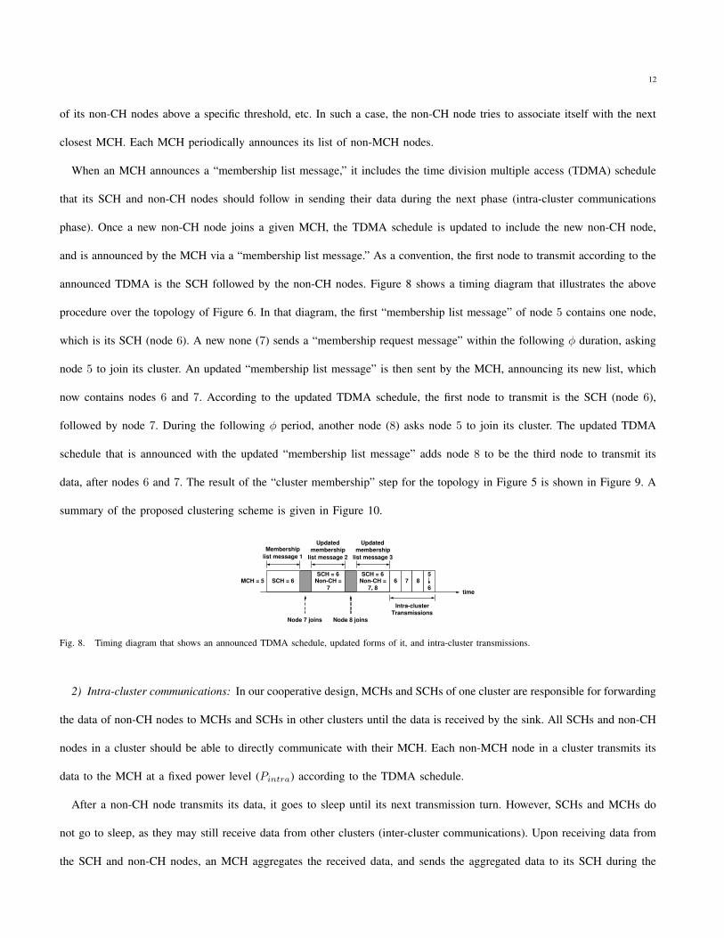
When an MCH announces a “membership list message,” it includes the time division multiple access (TDMA) schedule

that its SCH and non-CH nodes should follow in sending their data during the next phase (intra-cluster communications

phase). Once a new non-CH node joins a given MCH, the TDMA schedule is updated to include the new non-CH node,

and is announced by the MCH via a “membership list message.” As a convention, the first node to transmit according to the

announced TDMA is the SCH followed by the non-CH nodes. Figure 8 shows a timing diagram that illustrates the above

procedure over the topology of Figure 6. In that diagram, the first “membership list message” of node 5 contains one node,

which is its SCH (node 6). A new none (7) sends a “membership request message” within the following φ duration, asking

node 5 to join its cluster. An updated “membership list message” is then sent by the MCH, announcing its new list, which

now contains nodes 6 and 7. According to the updated TDMA schedule, the first node to transmit is the SCH (node 6),

followed by node 7. During the following φ period, another node (8) asks node 5 to join its cluster. The updated TDMA

schedule that is announced with the updated “membership list message” adds node 8 to be the third node to transmit its

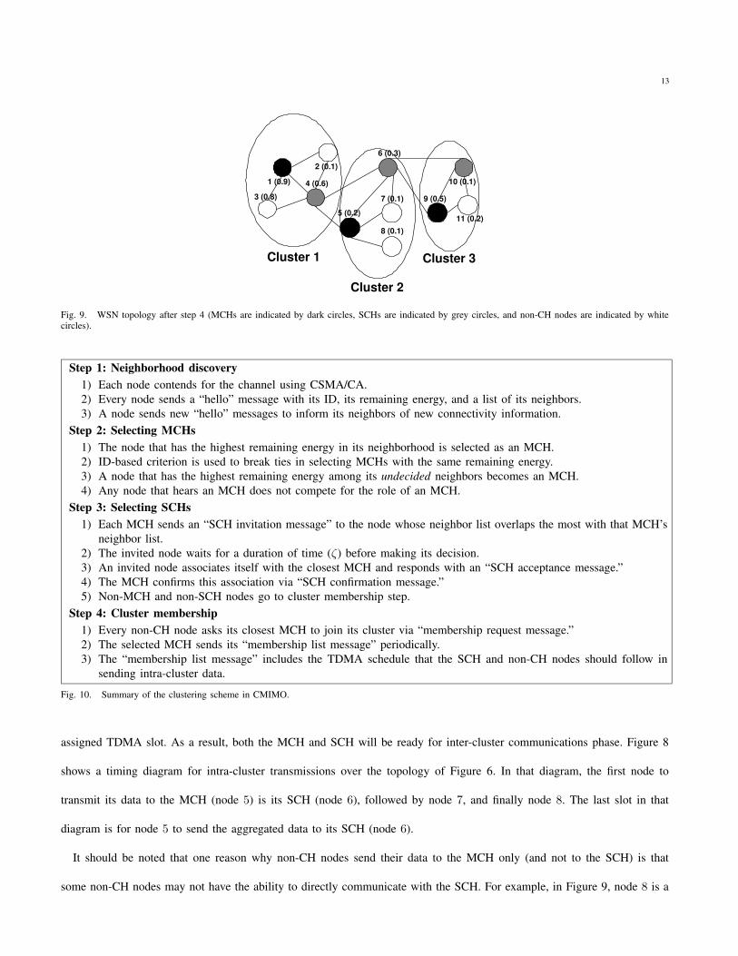
data, after nodes 6 and 7. The result of the “cluster membership” step for the topology in Figure 5 is shown in Figure 9. A

summary of the proposed clustering scheme is given in Figure 10.

MCH = 5

time

SCH = 6 SCH = 6

Non-CH = 7

SCH = 6 Non-CH =

7, 8

Membership list message 1

Updated membership

list message 2

Updated membership

list message 3

Node 7 joins Node 8 joins

6 7 8 5

6

Intra-cluster Transmissions

Fig. 8. Timing diagram that shows an announced TDMA schedule, updated forms of it, and intra-cluster transmissions.

2) Intra-cluster communications: In our cooperative design, MCHs and SCHs of one cluster are responsible for forwarding

the data of non-CH nodes to MCHs and SCHs in other clusters until the data is received by the sink. All SCHs and non-CH

nodes in a cluster should be able to directly communicate with their MCH. Each non-MCH node in a cluster transmits its

data to the MCH at a fixed power level (Pintra) according to the TDMA schedule.

After a non-CH node transmits its data, it goes to sleep until its next transmission turn. However, SCHs and MCHs do

not go to sleep, as they may still receive data from other clusters (inter-cluster communications). Upon receiving data from

the SCH and non-CH nodes, an MCH aggregates the received data, and sends the aggregated data to its SCH during the

13

Cluster 1

Cluster 2

Cluster 3

1 (0.9)

3 (0.8)

2 (0.1)

4 (0.6)

6 (0.3)

5 (0.2)

7 (0.1)

8 (0.1)

9 (0.5)

11 (0.2)

10 (0.1)

Fig. 9. WSN topology after step 4 (MCHs are indicated by dark circles, SCHs are indicated by grey circles, and non-CH nodes are indicated by whitecircles).

Step 1: Neighborhood discovery1) Each node contends for the channel using CSMA/CA.2) Every node sends a “hello” message with its ID, its remaining energy, and a list of its neighbors.3) A node sends new “hello” messages to inform its neighbors of new connectivity information.

Step 2: Selecting MCHs1) The node that has the highest remaining energy in its neighborhood is selected as an MCH.2) ID-based criterion is used to break ties in selecting MCHs with the same remaining energy.3) A node that has the highest remaining energy among its undecided neighbors becomes an MCH.4) Any node that hears an MCH does not compete for the role of an MCH.

Step 3: Selecting SCHs1) Each MCH sends an “SCH invitation message” to the node whose neighbor list overlaps the most with that MCH’s

neighbor list.2) The invited node waits for a duration of time (ζ) before making its decision.3) An invited node associates itself with the closest MCH and responds with an “SCH acceptance message.”4) The MCH confirms this association via “SCH confirmation message.”5) Non-MCH and non-SCH nodes go to cluster membership step.

Step 4: Cluster membership1) Every non-CH node asks its closest MCH to join its cluster via “membership request message.”2) The selected MCH sends its “membership list message” periodically.3) The “membership list message” includes the TDMA schedule that the SCH and non-CH nodes should follow in

sending intra-cluster data.

Fig. 10. Summary of the clustering scheme in CMIMO.

assigned TDMA slot. As a result, both the MCH and SCH will be ready for inter-cluster communications phase. Figure 8

shows a timing diagram for intra-cluster transmissions over the topology of Figure 6. In that diagram, the first node to

transmit its data to the MCH (node 5) is its SCH (node 6), followed by node 7, and finally node 8. The last slot in that

diagram is for node 5 to send the aggregated data to its SCH (node 6).

It should be noted that one reason why non-CH nodes send their data to the MCH only (and not to the SCH) is that

some non-CH nodes may not have the ability to directly communicate with the SCH. For example, in Figure 9, node 8 is a

14

non-CH node that cannot directly communicate with its SCH (node 6). However, by design all non-CH nodes must be able

to directly communicate with the MCH.

3) Inter-cluster communications with cooperative MIMO: Recall that the MCH and SCH in a cluster use adaptive

transmission mode and transmission power in communicating with MCHs and SCHs in other clusters by forming cooperative

MIMO nodes. We now discuss how to establish an inter-cluster virtual MIMO link. We consider two adjacent clusters. Each

cluster is represented by at most two CHs (MCH and SCH). We refer to the sending cluster as transmitting cluster, and

the cluster that is intended to receive data from the transmitting cluster as receiving cluster. The purpose of the following

steps is to decide on the appropriate MIMO mode to be used, and allow the CHs of the transmitting cluster to have enough

information that is needed in subsequent data transmissions between the transmitting and receiving clusters. The operational

details of establishing inter-cluster communications are explained in the following steps:

Step 1: An MCH in a given cluster accesses the channel using the CSMA/CA scheme. Once admitted, the MCH transmits

a request-to-send (RTS) packet at a fixed power level (Pinter) to the MCH and SCH (if any) in a next-hop cluster. The

purpose of this RTS packet is to notify the CHs of the receiving cluster that the SCH of the source cluster will be sending

another RTS packet. The MCH’s RTS should be heard by the SCH of the transmitting cluster, so that the latter knows when

to send its own RTS. Note that Pinter is chosen so that CMIMO produces a connected CH graph. Graph connectivity is

discussed in detail in section IV.

Step 2: The SCH of the transmitting cluster sends its RTS to the CHs (MCH and SCH) of the receiving cluster. This

RTS is sent at power level Pinter. It also serves as an indication to the transmitting MCH that the SCH has already heard

the MCH’s RTS, i.e., it is an implicit ACK from the SCH. An example that illustrates control-packet exchanges between

two clusters (steps 1 and 2) is shown in Figure 11.

SCH's RTS

MCH’s RTS

Transmitting cluster

Receiving cluster

Fig. 11. Control-packet exchanges between two clusters (MCHs are indicated by dark circles, whereas SCHs are indicated by grey circles).

15

Step 3: Upon receiving the two RTS packets from the transmitting MCH and SCH, respectively, the receiving MCH

and SCH estimate the channel gain between the CHs in the two clusters and communicate such information with each

other. From that, the receiving CHs calculate the required power that is needed to communicate between the CHs of the

transmitting and receiving clusters using one of four possible modes (SISO, MISO, SIMO, MIMO). Thus, four possible

modes are available for each inter-cluster hop along the end-to-end path. As explained later, mode selection is dictated by

energy-consumption considerations. Note that the 2 × 2 MIMO mode may not be a choice if there is no SCH at either

cluster of an inter-cluster link.

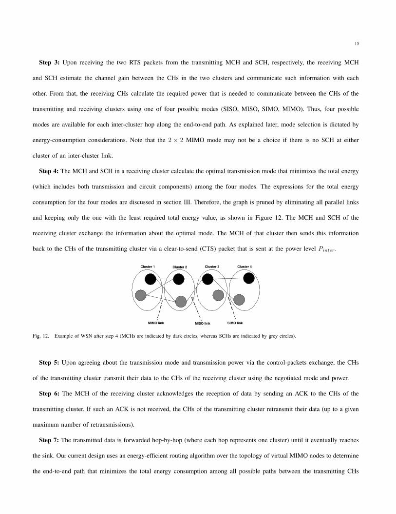
Step 4: The MCH and SCH in a receiving cluster calculate the optimal transmission mode that minimizes the total energy

(which includes both transmission and circuit components) among the four modes. The expressions for the total energy

consumption for the four modes are discussed in section III. Therefore, the graph is pruned by eliminating all parallel links

and keeping only the one with the least required total energy value, as shown in Figure 12. The MCH and SCH of the

receiving cluster exchange the information about the optimal mode. The MCH of that cluster then sends this information

back to the CHs of the transmitting cluster via a clear-to-send (CTS) packet that is sent at the power level Pinter.

MIMO link MISO link SIMO link

Cluster 1 Cluster 2 Cluster 3 Cluster 4

Fig. 12. Example of WSN after step 4 (MCHs are indicated by dark circles, whereas SCHs are indicated by grey circles).

Step 5: Upon agreeing about the transmission mode and transmission power via the control-packets exchange, the CHs

of the transmitting cluster transmit their data to the CHs of the receiving cluster using the negotiated mode and power.

Step 6: The MCH of the receiving cluster acknowledges the reception of data by sending an ACK to the CHs of the

transmitting cluster. If such an ACK is not received, the CHs of the transmitting cluster retransmit their data (up to a given

maximum number of retransmissions).

Step 7: The transmitted data is forwarded hop-by-hop (where each hop represents one cluster) until it eventually reaches

the sink. Our current design uses an energy-efficient routing algorithm over the topology of virtual MIMO nodes to determine

the end-to-end path that minimizes the total energy consumption among all possible paths between the transmitting CHs

16

and the sink. This algorithm consists of two steps. In the first step, all pairs of virtual MIMO nodes that can communicate

directly at power Pinter using at least one of the four transmission modes are determined. For a given pair, we establish as

many parallel links as the number of feasible transmission modes between the two virtual MIMO nodes. We then prune the

graph and keep only the one with the least required total energy (transmission plus circuit) value. In the second step of the

algorithm, we run a modified version of Dijkstra’s algorithm, where the weight of a link is taken as its total energy value

determined from the first step. The returned path has the minimum sum of total energy values among all possible paths

between the transmitting CHs and the sink.

Its should be noted that the MCH (or both MCH and SCH) of the receiving cluster selects the optimal transmission

mode and transmission power for communication with other CHs. The mode and power can be different for different hops,

depending on the distances between CHs in different clusters. We now discuss how the sink can know about the most

energy-efficient path between the transmitting CHs and itself. The key idea here is that when an MCH sends its “SCH

confirmation message” to its own non-MCH nodes and also to other neighboring MCHs, such a message is also flooded by

neighboring MCHs. This way, the sink will eventually learn about the various MCH nodes. The sink can then determine

the optimal route (based on the total energy values) from every MCH to itself, and can inform every MCH with its next

inter-cluster hop (in one message that is flooded throughout the network). As a result, an MCH with data to send knows

the next hop to the sink.

C. Properties of CMIMO

CMIMO has several features. First, it is completely distributed. This is because every node in the WSN independently

takes its decisions based on local information. Second, at the end of the clustering process, a node is either a CH (master

or slave) or a non-CH node that belongs to a cluster. In other words, the clustering process is guaranteed to terminate. This

can be easily proven by noting that the node within the highest remaining energy in its neighborhood is elected as an MCH.

Such an MCH then selects an SCH according to the neighbor list criterion. Next, each non-CH node selects one of the

MCHs to join. Third, an SCH cannot belong to more than one cluster. This is because an invited SCH responds to only

one of the received requests from MCHs. Fourth, the probability that two nodes within each other’s cluster range are both

MCHs is zero, i.e., MCHs are well distributed. This is attributed to the fact that MCHs are selected in an iterative manner

and using a real-valued parameter (remaining energy).

17

III. ENERGY MODEL

In this section, we analyze the energy consumption model of the CMIMO scheme. The purpose of this analysis is to

study the tradeoff between various parameters that are used in the system design, as well as to obtain the energy values

of the four possible transmission modes for the protocol operation. Following [4], the total power consumed for sending a

packet consists of transmission and circuit powers. The transmission power for inter-cluster data transmissions is adjustable

and is given by Pt = (1 + δ)Pout, where δ is a factor that depends on the drain efficiency [14] of the power amplifier and

the underlying modulation scheme [12], and Pout is the total transmit power at the air interface. This Pout can be expressed

as:

Pout = γ(Mt,Mr)NoBNfGoMldn (1)

where γ(Mt,Mr) is the required SNR at the receiver when Mt and Mr antennas are used for transmission and reception,

respectively, No is the single-sided thermal noise power spectral density (PSD), B is the passband bandwidth, Nf is the

receiver noise figure (Nfdef= Nr

No

, with Nr being the PSD of the total effective noise at the receiver input), Go is a constant

that depends on the transmitter and receiver antenna gains, Ml is a link margin that compensates for hardware variations and

other sources of interference, n is the path-loss exponent, and d is the transmitter-receiver distance. Note that γ(Mt,Mr)

depends on the target BER and the specific transmission mode.

As for the circuit power (Pc), it is given by [4]:

Pc ≈ Mt(PDAC + Pmix + Pfilt) + 2Psyn+

Mr(PLNA + Pmix + PIFA + Pfilr + PADC) (2)

where PDAC , Pmix, PLNA, PIFA, Pfilt, Pfilr, PADC , and Psyn are the power consumption values for the digital-to-analog

converter, the mixer, the low noise amplifier, the intermediate frequency amplifier, the active filters at the transmitter and

the receiver sides, the analog-to-digital converter, and the frequency synthesizer, respectively.

Accordingly, the total energy consumption per bit is:

Ebt =Pt + Pc

Rb

(3)

18

where Rb is the bit rate. Using (1) and (2), Ebt can be written in terms of d, Mt, Mr, and Rb as follows:

Ebt =C1γ(Mt,Mr)d

n + C2Mt + C3Mr + C4

Rb

(4)

where C1, C2, C3, and C4 are circuit-specific constants.

Note that the transmission mode defined by (Mt and Mr), γ(Mt,Mr), and d have significant impacts on Ebt. For the

same value of BER, the smaller the values of Mt and Mr, the larger the γ(Mt,Mr), i.e., γ(1, 1) > γ(2, 2), making MIMO

more favorable in terms of transmission power [12]. However, a distance-dependent tradeoff emerges between transmission

and circuit powers. Whereas multi-antenna transmission requires less transmission power than, say, a SISO system for the

same target BER, it also requires more circuit power at both ends of the link. For relatively small distances, circuit power is

dominant, and hence a SISO mode is more energy-efficient than a multi-antenna mode. As the transmitter-receiver distance

increases, the tradeoff shifts in favor of multi-antenna modes (SIMO, MISO, MIMO). As a result, one of the four possible

modes becomes more favorable for an inter-cluster communication.

IV. CMIMO DESIGN ISSUES

In this section, we discuss some issues related to the design of CMIMO. These include connectivity, listening cost,

synchronization, reclustering, and MAC.

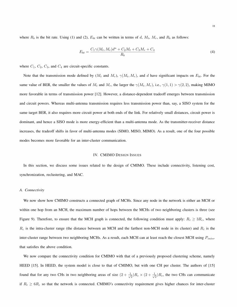
A. Connectivity

We now show how CMIMO constructs a connected graph of MCHs. Since any node in the network is either an MCH or

within one hop from an MCH, the maximum number of hops between the MCHs of two neighboring clusters is three (see

Figure 9). Therefore, to ensure that the MCH graph is connected, the following condition must apply: Rt ≥ 3Rc, where

Rc is the intra-cluster range (the distance between an MCH and the farthest non-MCH node in its cluster) and Rt is the

inter-cluster range between two neighboring MCHs. As a result, each MCH can at least reach the closest MCH using Pinter

that satisfies the above condition.

We now compare the connectivity condition for CMIMO with that of a previously proposed clustering scheme, namely

HEED [15]. In HEED, the system model is close to that of CMIMO, but with one CH per cluster. The authors of [15]

found that for any two CHs in two neighboring areas of size (2 + 1√2)Rc × (2 + 1√

2)Rc, the two CHs can communicate

if Rt ≥ 6Rc so that the network is connected. CMIMO’s connectivity requirement gives higher chances for inter-cluster

19

MCHs to take place than HEED, as a smaller range is reserved for inter-cluster communications (i.e., there is more spatial

reuse).

B. Listening Cost

We now discuss several approaches that can be used by CMIMO to reduce the listening cost of active nodes. To ensure

inter-cluster routing, MCHs and SCHs should always be available. On the other hand, non-CH nodes can be put to sleep after

they send their data to their MCHs. CHs can also follow some duty cycle to reduce their energy consumption, as follows.

When a packet is intended to a CH, the CH should wakeup for a duration of time that is needed to receive the coming

data. This, however, requires coordination between the CH and its non-CH nodes. Several general-purpose approaches for

coordinating communications can be used in this context, such as S-MAC [16], T-MAC [17], and TRAMA [18].

C. Synchronization

Extensive research has been done on quantifying the tradeoff between implementing synchronous network operation

and the overhead and inaccuracy associated with such operation. Our CMIMO design can be in either synchronous or

asynchronous modes.

Several approaches were proposed to solve the synchronization issue. One of them suggests using a reference-broadcast

synchronization (RBS) technique [19], which we can adapt to CMIMO as follows. An MCH asks one of its cluster nodes

(except the SCH) to send RBS beacons. After exchanging the RBS beacons, the MCH and SCH start sending the data

simultaneously to the CHs in a receiving cluster. Another approach is to use the transmission delay and channel estimation

scheme proposed in [5]. The main drawbacks of these approaches are the large number of generated messages, the long

elapsed time in overall synchronization, and that they do not consider the energy requirement of sensor nodes.

To overcome the above drawbacks, we now give an overview of our proposed solution to the synchronization issue.

The key idea is to select a node in the network to act as a beacon cluster head (BCH). Such a node sends beacons to its

neighboring MCHs so that they adjust the start time of their frames accordingly. The only condition for this node is to be an

MCH, as it mainly communicates with neighboring MCHs. To satisfy this condition, one node is arbitrarily chosen during

the design phase (before starting the “cluster formation” phase) to be a BCH. After MCHs are selected, two possibilities

may exist regarding the selected BCH node. First, the selected BCH may happen to be an MCH. Accordingly, this node

acts as a BCH. Second, the selected BCH may happen to be a non-MCH node (SCH or non-CH node). In such a case, the

20

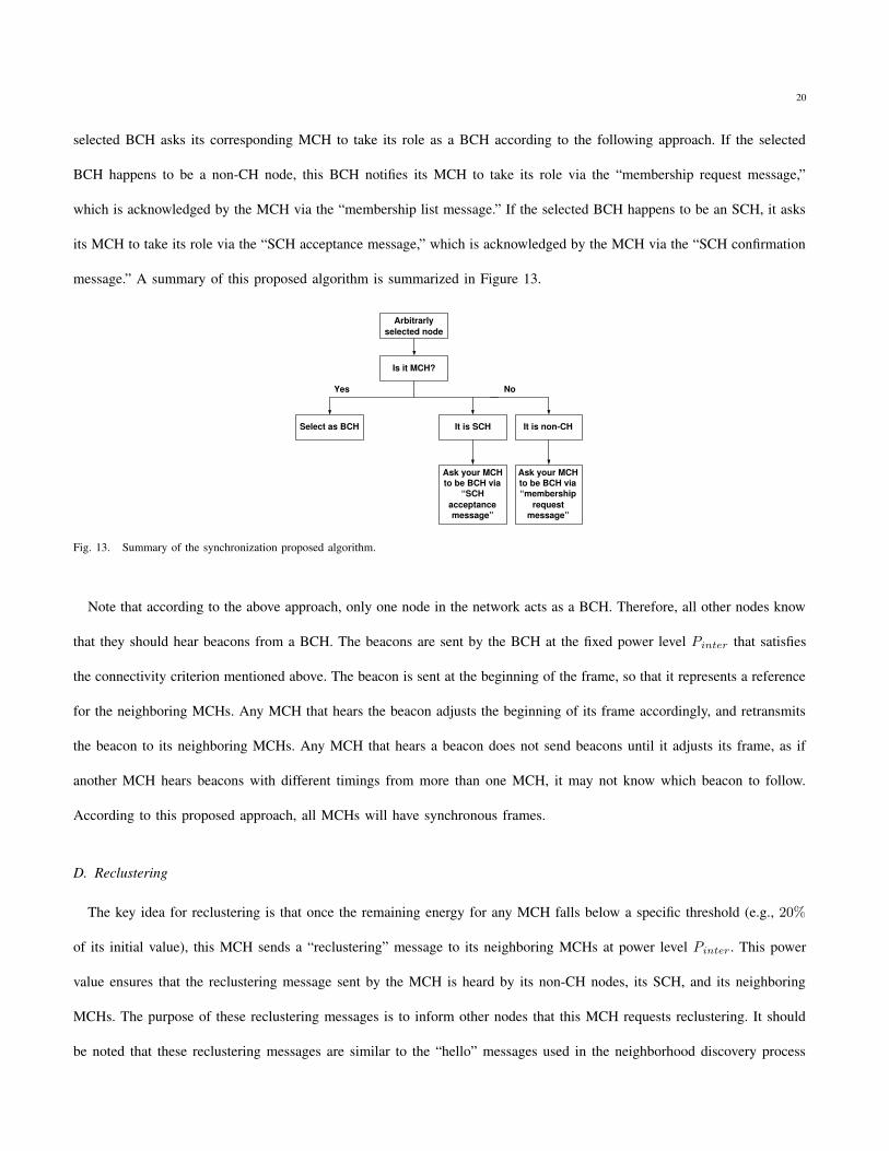
selected BCH asks its corresponding MCH to take its role as a BCH according to the following approach. If the selected

BCH happens to be a non-CH node, this BCH notifies its MCH to take its role via the “membership request message,”

which is acknowledged by the MCH via the “membership list message.” If the selected BCH happens to be an SCH, it asks

its MCH to take its role via the “SCH acceptance message,” which is acknowledged by the MCH via the “SCH confirmation

message.” A summary of this proposed algorithm is summarized in Figure 13.

Arbitrarly selected node

Is it MCH?

It is SCH Select as BCH

Yes No

It is non-CH

Ask your MCH to be BCH via

“SCH acceptance message”

Ask your MCH to be BCH via “membership

request message”

Fig. 13. Summary of the synchronization proposed algorithm.

Note that according to the above approach, only one node in the network acts as a BCH. Therefore, all other nodes know

that they should hear beacons from a BCH. The beacons are sent by the BCH at the fixed power level Pinter that satisfies

the connectivity criterion mentioned above. The beacon is sent at the beginning of the frame, so that it represents a reference

for the neighboring MCHs. Any MCH that hears the beacon adjusts the beginning of its frame accordingly, and retransmits

the beacon to its neighboring MCHs. Any MCH that hears a beacon does not send beacons until it adjusts its frame, as if

another MCH hears beacons with different timings from more than one MCH, it may not know which beacon to follow.

According to this proposed approach, all MCHs will have synchronous frames.

D. Reclustering

The key idea for reclustering is that once the remaining energy for any MCH falls below a specific threshold (e.g., 20%

of its initial value), this MCH sends a “reclustering” message to its neighboring MCHs at power level Pinter. This power

value ensures that the reclustering message sent by the MCH is heard by its non-CH nodes, its SCH, and its neighboring

MCHs. The purpose of these reclustering messages is to inform other nodes that this MCH requests reclustering. It should

be noted that these reclustering messages are similar to the “hello” messages used in the neighborhood discovery process

21

in step 1 of the “cluster formation” phase, except that the reclustering messages are sent at a higher power level (Pinter).

As a result, the neighboring MCHs that hear these messages respond as in the previously discussed neighborhood discovery

process. The rationale behind restricting the reclustering request to MCHs is that in most cases, MCHs are the ones that

deplete their batteries first (before SCHs and non-CH nodes), as MCHs are responsible for aggregating data, sending it to

the SCH, and forwarding it to CHs in neighboring clusters.

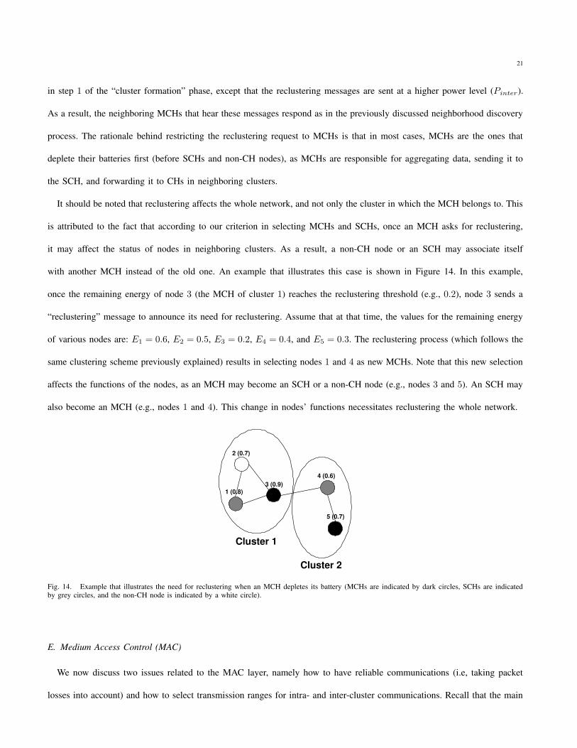
It should be noted that reclustering affects the whole network, and not only the cluster in which the MCH belongs to. This

is attributed to the fact that according to our criterion in selecting MCHs and SCHs, once an MCH asks for reclustering,

it may affect the status of nodes in neighboring clusters. As a result, a non-CH node or an SCH may associate itself

with another MCH instead of the old one. An example that illustrates this case is shown in Figure 14. In this example,

once the remaining energy of node 3 (the MCH of cluster 1) reaches the reclustering threshold (e.g., 0.2), node 3 sends a

“reclustering” message to announce its need for reclustering. Assume that at that time, the values for the remaining energy

of various nodes are: E1 = 0.6, E2 = 0.5, E3 = 0.2, E4 = 0.4, and E5 = 0.3. The reclustering process (which follows the

same clustering scheme previously explained) results in selecting nodes 1 and 4 as new MCHs. Note that this new selection

affects the functions of the nodes, as an MCH may become an SCH or a non-CH node (e.g., nodes 3 and 5). An SCH may

also become an MCH (e.g., nodes 1 and 4). This change in nodes’ functions necessitates reclustering the whole network.

Cluster 1

Cluster 2

1 (0.8)

4 (0.6) 3 (0.9)

5 (0.7)

2 (0.7)

Fig. 14. Example that illustrates the need for reclustering when an MCH depletes its battery (MCHs are indicated by dark circles, SCHs are indicatedby grey circles, and the non-CH node is indicated by a white circle).

E. Medium Access Control (MAC)

We now discuss two issues related to the MAC layer, namely how to have reliable communications (i.e, taking packet

losses into account) and how to select transmission ranges for intra- and inter-cluster communications. Recall that the main

22

emphasis of our work is on the clustering/routing aspects of cooperative MIMO, which take place in layers that are above

the MAC layer.

Reliable communication is established by using ACKs at the MAC layer for all network transmissions. These include

transmissions for neighborhood discovery (where hello messages represent implicit ACKs for previously heard hello mes-

sages), between a non-CH node and its MCH (e.g., a “membership request message” is acknowledged by a “membership list

message”), between an SCH and its MCH (e.g., an “SCH acceptance message” is acknowledged by an “SCH confirmation

message”), and between an SCH/MCH in a transmitting cluster and an SCH/MCH in a receiving cluster (e.g., MCH’s

and SCH’s RTSs are acknowledged by MCH’s CTS). In addition, CMIMO retransmits the packets that have not been

acknowledged (limited to a specific number of retransmissions) to increase the chances of correctly receiving these packets.

For selecting transmission ranges, one approach is to use code division multiple access (CDMA) technique [20], where

different coding schemes for intra- and inter-cluster transmissions are used. However, the hardware implications of such

a technique may render it infeasible. Therefore, we propose another approach, in which the transmission range of inter-

cluster communications (Rt) is selected a priori. The intra-cluster range is then selected so that the connectivity condition

(Rt ≥ 3Rc) is satisfied. We argue that this approach has less complexity than the CDMA approach.

V. PERFORMANCE EVALUATION

In this section, we evaluate the performance of CMIMO via simulations. We also compare it with the DCA scheme [21],

which is one of the fundamental clustering schemes. The purpose of choosing DCA to compare our scheme with is that

DCA resembles CMIMO in the criterion used to select CHs. Also, the primary goal of this comparison is to demonstrate

the benefits of using cooperative MIMO over a single-antenna system (DCA). Recall that CMIMO adapts the transmission

mode and transmission power on a per-packet basis. On the other hand, all transmissions in DCA take place using the SISO

mode, where each cluster has only one CH.

For both CMIMO and DCA, we use the following simulations setup, unless stated otherwise. We consider 100 nodes that

are uniformly deployed within a square of 1000 meter × 1000 meter. The sink is located outside (to the right of) the square

field. Each node generates packets according to a Poisson process of rate λ3. The sink is the only node that is equipped

with two antennas. The rationale behind this design is to achieve MIMO gain for the last hop. Multi-hop operation based on

an energy-efficient routing is used for inter-cluster communications. The values of γ(Mt,Mr) that are required to achieve a

3Other traffic models, such as Markov-modulated Poisson process (MMPP), can also be used by CMIMO to generate packets.

23

TABLE IIISIMULATION PARAMETERS

Data-packets size 2000 bytesControl-packets size 20 bytes

Rb 1 Mbpsλ 20 packets/sec

PDAC 15 mWPADC 15 mWPmix 30.3 mWPfilt 2.5 mWPfilr 2.5 mWPsyn 50 mWPLNA 20 mWPIFA 2 mWMl 10 dBNf 10 dB

BER of 0.001 are taken from [4]: 24.4 dB for SISO, 10.6 dB for SIMO, 14.1 dB for MISO, and 6.9 dB for MIMO. For the

wireless channel, we assume Rayleigh fading model along with a distance-dependent path loss, which has a power falloff

of d4. Intra-cluster range (Rc) is set to 60 meters, and inter-cluster range (Rt) is set based on the connectivity condition

(Rt = 3Rc). For figures that vary either Rc or Rt, the other range is still determined based on the connectivity condition.

Other simulation parameters are given in Table III. We repeated each experiment 100 times with different seed numbers

and averaged the results. The confidence intervals were sufficiently tight, and are not shown to prevent cluttering the plots.

Our results are based on simulation experiments conducted using CSIM programs (CSIM is a C-based process-oriented

discrete-event simulation package [22]). The primary performance metrics are energy consumption, network throughput, the

fraction of time that each transmission mode is used, and the percentage of number of hops.

A. Energy Consumption

Figure 15 shows the impact of inter-cluster range (the maximum range for direct communications between two clusters)

on the total energy consumption for CMIMO and DCA. Such a range is controlled via Pinter. The results illustrate that

the total energy consumption increases with the inter-cluster range. CMIMO outperforms DCA in energy consumption. The

superiority of CMIMO over DCA becomes more significant as the inter-cluster range increases. The reason is that increasing

the inter-cluster range forces clusters that are far away from each other to communicate using multi-antenna modes. In this

case, the transmission energy dominates the circuit energy, making MIMO/MISO/SIMO more energy-efficient than the SISO

mode. Thus, exploiting cooperative MIMO systems is more energy-efficient under large inter-cluster ranges.

24

500 550 600 650 700 750 800 850 9000

0.005

0.01

0.015

0.02

0.025

0.03

0.035

0.04

0.045

Inter−Cluster Range (meters)

Tota

l Ene

rgy

Con

sum

ptio

n (J

oule

s/bi

t)

CMIMODCA

Fig. 15. Energy consumption per bit versus inter-cluster range.

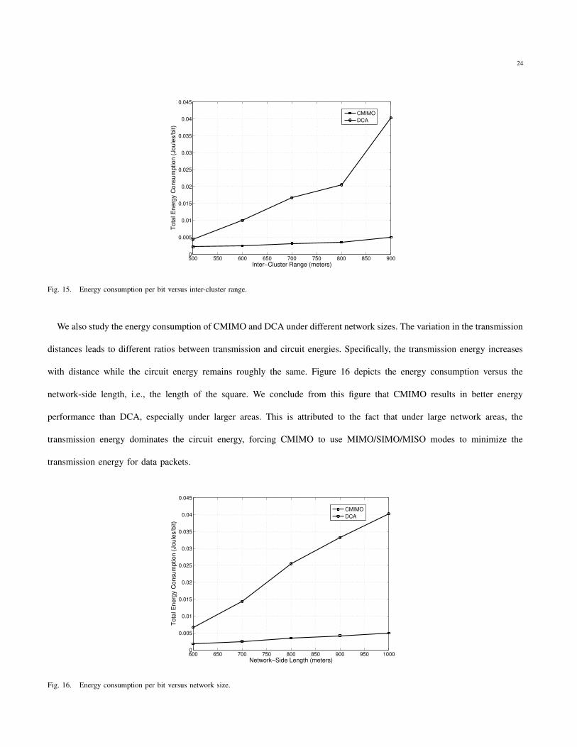
We also study the energy consumption of CMIMO and DCA under different network sizes. The variation in the transmission

distances leads to different ratios between transmission and circuit energies. Specifically, the transmission energy increases

with distance while the circuit energy remains roughly the same. Figure 16 depicts the energy consumption versus the

network-side length, i.e., the length of the square. We conclude from this figure that CMIMO results in better energy

performance than DCA, especially under larger areas. This is attributed to the fact that under large network areas, the

transmission energy dominates the circuit energy, forcing CMIMO to use MIMO/SIMO/MISO modes to minimize the

transmission energy for data packets.

600 650 700 750 800 850 900 950 10000

0.005

0.01

0.015

0.02

0.025

0.03

0.035

0.04

0.045

Network−Side Length (meters)

Tota

l Ene

rgy

Con

sum

ptio

n (J

oule

s/bi

t)

CMIMODCA

Fig. 16. Energy consumption per bit versus network size.

25

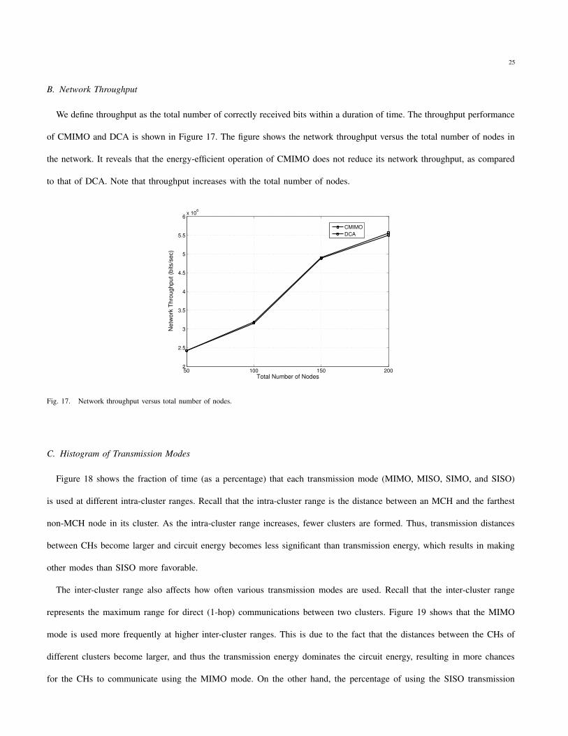
B. Network Throughput

We define throughput as the total number of correctly received bits within a duration of time. The throughput performance

of CMIMO and DCA is shown in Figure 17. The figure shows the network throughput versus the total number of nodes in

the network. It reveals that the energy-efficient operation of CMIMO does not reduce its network throughput, as compared

to that of DCA. Note that throughput increases with the total number of nodes.

50 100 150 2002

2.5

3

3.5

4

4.5

5

5.5

6x 10

6

Total Number of Nodes

Net

wor

k Th

roug

hput

(bits

/sec

)

CMIMODCA

Fig. 17. Network throughput versus total number of nodes.

C. Histogram of Transmission Modes

Figure 18 shows the fraction of time (as a percentage) that each transmission mode (MIMO, MISO, SIMO, and SISO)

is used at different intra-cluster ranges. Recall that the intra-cluster range is the distance between an MCH and the farthest

non-MCH node in its cluster. As the intra-cluster range increases, fewer clusters are formed. Thus, transmission distances

between CHs become larger and circuit energy becomes less significant than transmission energy, which results in making

other modes than SISO more favorable.

The inter-cluster range also affects how often various transmission modes are used. Recall that the inter-cluster range

represents the maximum range for direct (1-hop) communications between two clusters. Figure 19 shows that the MIMO

mode is used more frequently at higher inter-cluster ranges. This is due to the fact that the distances between the CHs of

different clusters become larger, and thus the transmission energy dominates the circuit energy, resulting in more chances

for the CHs to communicate using the MIMO mode. On the other hand, the percentage of using the SISO transmission

26

60 100 140 1800

10

20

30

40

50

60

70

80

Intra−Cluster Range (meters)

Per

cent

age

of T

rans

mis

sion

Mod

e

MIMOMISOSIMOSISO

Fig. 18. Percentage of transmission modes versus intra-cluster range.

mode decreases as the inter-cluster range increases.

500 600 700 800 9000

10

20

30

40

50

60

70

Inter−Cluster Range (meters)

Per

cent

age

of T

rans

mis

sion

Mod

e

MIMOMISOSIMOSISO

Fig. 19. Percentage of transmission modes versus inter-cluster range.

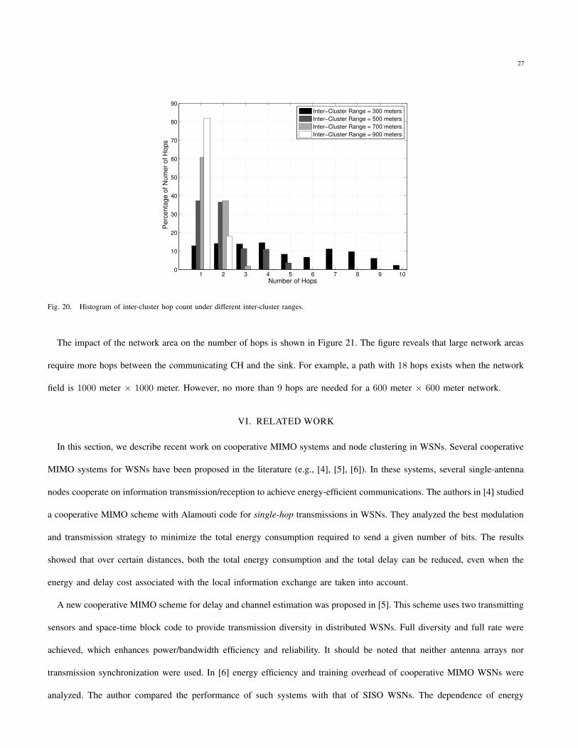
D. Number of Hops

We now study the impact of inter-cluster range and network area on the number of hops used for inter-cluster commu-

nications to the sink. Figure 20 shows a histogram of the number of hops needed for routing under different inter-cluster

ranges. As expected, under small inter-cluster ranges (e.g., 300 meters), routes with large numbers of hops exist (10 hops).

On the other hand, when the inter-cluster range becomes large (e.g., 900 meters), fewer hops are needed (2 hops).

27

1 2 3 4 5 6 7 8 9 100

10

20

30

40

50

60

70

80

90

Number of Hops

Per

cent

age

of N

umer

of H

ops

Inter−Cluster Range = 300 metersInter−Cluster Range = 500 metersInter−Cluster Range = 700 metersInter−Cluster Range = 900 meters

Fig. 20. Histogram of inter-cluster hop count under different inter-cluster ranges.

The impact of the network area on the number of hops is shown in Figure 21. The figure reveals that large network areas

require more hops between the communicating CH and the sink. For example, a path with 18 hops exists when the network

field is 1000 meter × 1000 meter. However, no more than 9 hops are needed for a 600 meter × 600 meter network.

VI. RELATED WORK

In this section, we describe recent work on cooperative MIMO systems and node clustering in WSNs. Several cooperative

MIMO systems for WSNs have been proposed in the literature (e.g., [4], [5], [6]). In these systems, several single-antenna

nodes cooperate on information transmission/reception to achieve energy-efficient communications. The authors in [4] studied

a cooperative MIMO scheme with Alamouti code for single-hop transmissions in WSNs. They analyzed the best modulation

and transmission strategy to minimize the total energy consumption required to send a given number of bits. The results

showed that over certain distances, both the total energy consumption and the total delay can be reduced, even when the

energy and delay cost associated with the local information exchange are taken into account.

A new cooperative MIMO scheme for delay and channel estimation was proposed in [5]. This scheme uses two transmitting

sensors and space-time block code to provide transmission diversity in distributed WSNs. Full diversity and full rate were

achieved, which enhances power/bandwidth efficiency and reliability. It should be noted that neither antenna arrays nor

transmission synchronization were used. In [6] energy efficiency and training overhead of cooperative MIMO WSNs were

analyzed. The author compared the performance of such systems with that of SISO WSNs. The dependence of energy

28

0 1 2 3 4 5 6 7 8 9 10 11 12 13 14 15 16 17 180

5

10

15

20

25

Number of Hops

Per

cent

age

of N

umbe

r of H

ops

Network−Side Length = 600 metersNetwork−Side Length = 700 metersNetwork−Side Length = 800 metersNetwork−Side Length = 900 metersNetwork−Side Length = 1000 meters

Fig. 21. Histogram of inter-cluster hop count under different network areas.

efficiency on the coherence time of the fading process and on the communications distance was considered.

In all the above-mentioned contributions, clustering and multi-hop routing were not taken into consideration, which limits

the scalability of these schemes in large WSNs.

Many clustering schemes were proposed for WSNs, which can be classified based on two criteria [23]: (1) the parameters

used for electing CHs, and (2) the execution nature of the clustering algorithm (probabilistic or iterative). Some clustering

schemes under the first category use the node ID to elect CHs. Others favor nodes with larger degrees. Some other schemes

were proposed for controlling the network topology by exploiting node redundancy. Regarding the second category, the

execution of a clustering scheme can be carried out at a centralized authority (e.g., a base station) or in a distributed way

at local nodes. In iterative clustering schemes, a node waits for a specific event to occur or certain nodes to decide their

role (e.g., become CHs) before making a decision. This results in some delay in the convergence time. On the other hand,

probabilistic (or randomized) clustering schemes ensure rapid convergence while achieving some favorable properties, such

as balanced cluster sizes.

One of the fundamental clustering schemes is the distributed clustering algorithm (DCA) [21], which clusters nodes in an

iterative way. In DCA, nodes divide themselves into groups according to a weight-based criterion. The main assumptions

behind DCA are: (1) the network topology is static, and (2) each transmitted message is correctly received by all neighbors

within a specific duration of time. As the first assumption is reasonable for WSNs, the second one opens several issues

29

about reliability and how such a scheme can deal with collisions. The key idea in DCA is that a node decides its role in

the network after it hears the decisions of its neighbors that have higher weights.

HEED [15] is a clustering scheme that does not make any assumptions about the presence of infrastructure or about

node capabilities, other than the availability of multiple power levels in sensor nodes. The key idea behind this scheme

is to periodically select CHs according to a hybrid metric that combines the node’s remaining energy and a secondary

parameter, such as node proximity to its neighbors or node degree. The authors showed that with appropriate bounds on

node density and intra/inter-cluster transmission ranges, HEED can asymptotically almost surely guarantee connectivity of

clustered networks.

The authors in [2] developed a low-energy adaptive clustering hierarchy (LEACH), which combines the ideas of energy-

efficient cluster-based routing and medium access together with application-specific data aggregation, so as to improve the

performance in terms of system lifetime, latency, and application-perceived quality. LEACH enables self-organization of

large numbers of nodes, adapts clusters, and rotates CH role to evenly distribute the energy load among all the nodes.

It should be noted that all of these clustering schemes do not exploit cooperative MIMO with clustering. Moreover,

some of these schemes do not consider multi-hop communications and early data aggregation to save energy. On the other

hand, CMIMO is a cooperative-MIMO based scheme, where the decisions of the nodes that follow CMIMO are based on

MIMO-related parameters. Moreover, multi-hop operation and early data aggregation are considered in our design.

The authors in [24] extended the LEACH scheme to build a cluster-based cooperative MIMO scheme for WSNs, namely

MIMO-LEACH. The main differences between CMIMO and MIMO-LEACH can be summarized as follows. First, MIMO-

LEACH is based on an existing clustering scheme (LEACH) that does not take into account MIMO operations in the

clustering process, whereas CMIMO has its own clustering scheme that exploits MIMO operations in its selecting criteria.

Second, MIMO-LEACH contains one CH per cluster, which is responsible for aggregating data, and broadcasting it to two

other “cooperative” nodes. These nodes are responsible for forwarding the data to the CH of a receiving cluster. It is clear

that in [24], three nodes (one CH and two cooperative nodes) are needed to aggregate and forward the data, whereas only

the two CHs (MCH and SCH) are the ones that perform these functions in CMIMO. As a result, MIMO-LEACH involves

more overhead than CMIMO. Finally, four transmission modes are available in CMIMO for each link between any two

clusters. However, in MIMO-LEACH no complete MIMO communications (2 × 2) exist among the network, as the best

transmission mode that can be used is SIMO/MISO.

30

VII. CONCLUSIONS AND FUTURE EXTENSIONS

In this paper, we proposed a distributed and adaptive clustering/routing scheme (CMIMO) to minimize the total energy

consumption for a multi-hop WSN. CMIMO produces clusters that have two CHs, which are responsible for routing traffic

between clusters (i.e., inter-cluster communications). The proposed CMIMO scheme has the ability to adapt the transmission

mode (SISO, MISO, SIMO, MIMO) and the transmission power on a per-packet basis for inter-cluster transmissions. We

studied the performance of the CMIMO scheme via simulations. The results indicate that the proposed scheme achieves a

significant improvement in the overall energy consumption of the network compared to non-adaptive WSNs that are designed

with one CH per cluster and using SISO mode (e.g., WSNs under the DCA scheme). The significance of CMIMO becomes

more attractive under high intra/inter-cluster ranges and network sizes. CMIMO supports multi-hop scenarios and performs

better when the number of hops increases.

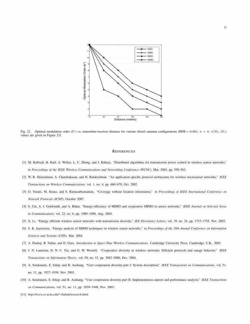
One possible extension to our work is to study the impact of the modulation order (b) on the total energy consumption.

The value of b represents the number of bits per symbol, which varies with the modulation scheme. For example, b = 1 for

binary-phase-shift keying (BPSK), b = 2 for quadrature-phase-shift keying (QPSK), etc.

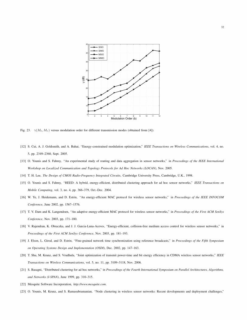
It was shown [12] that b impacts the energy consumption through γ(Mt,Mr), which itself depends on the target BER,

the specific transmission mode, and the transmission rate. As shown in Figure 23 [4], a higher value of b necessitates a

higher γ(Mt,Mr), i.e., more transmission power is required. However, it also means a higher transmission rate, i.e., lower

transmission time, which in turn reduces the energy consumption. The confluence of the two effects determines the optimal

modulation order (b∗). As shown in Figure 22, b∗ generally decreases with the transmitter-receiver distance, as transmission

energy becomes more dominant.

As previously mentioned, MIMO offers three types of gains: diversity, array, and multiplexing. In this work, we mainly

focused on the diversity gain. However, we plan on exploiting the other gains in future research. Our goal is to combine

different types of MIMO gains, allowing for dynamic switching between diversity, array, and multiplexing modes, so as to

maximize a utility function that depends on both energy consumption and throughput.

Although we only considered cooperative MIMO with two CHs per cluster, our design can be in principle extended to

higher-order MIMO systems. Note that going beyond 2× 2 systems (e.g. three CHs per cluster; MCH1, SCH1, and SCH2),

results in more overhead on intra-cluster part. As a result, it is not clear if adding more CHs per cluster improves the overall

performance compared to that of 2 × 2 systems. This issue is left to future work.

31

10 40 70 100 130 1601

2

3

4

5

6

7

8

9

10

11

12

Distance (meters)

Opt

imal

Mod

ulat

ion

Ord

er (b

*)

SISO

SIMO

MISO

MIMO

Fig. 22. Optimal modulation order (b∗) vs. transmitter-receiver distance for various (fixed) antenna configurations (BER = 0.001, n = 4, γ(Mt, Mr)values are given in Figure 23).

REFERENCES

[1] M. Kubisch, H. Karl, A. Wolisz, L. C. Zhong, and J. Rabaey, “Distributed algorithms for transmission power control in wireless sensor networks,”

in Proceedings of the IEEE Wireless Communications and Networking Conference (WCNC), Mar. 2003, pp. 558–563.

[2] W. R. Heinzelman, A. Chandrakasan, and H. Balakrishnan, “An application-specific protocol architecture for wireless microsensor networks,” IEEE

Transactions on Wireless Communications, vol. 1, no. 4, pp. 660–670, Oct. 2002.

[3] O. Younis, M. Krunz, and S. Ramasubramanian, “Coverage without location information,” in Proceedings of IEEE International Conference on

Network Protocols (ICNP), October 2007.

[4] S. Cui, A. J. Goldsmith, and A. Bahai, “Energy-efficiency of MIMO and cooperative MIMO in sensor networks,” IEEE Journal on Selected Areas

in Communications, vol. 22, no. 6, pp. 1089–1098, Aug. 2004.

[5] X. Li, “Energy efficient wireless sensor networks with transmission diversity,” IEE Electronics Letters, vol. 39, no. 24, pp. 1753–1755, Nov. 2003.

[6] S. K. Jayaweera, “Energy analysis of MIMO techniques in wireless sensor networks,” in Proceedings of the 38th Annual Conference on Information

Sciences and Systems (CISS), Mar. 2004.

[7] A. Paulraj, R. Nabar, and D. Gore, Introduction to Space-Time Wireless Communications, Cambridge University Press, Cambridge, U.K., 2003.

[8] J. N. Laneman, D. N. C. Tse, and G. W. Wornell, “Cooperative diversity in wireless networks: Efficient protocols and outage behavior,” IEEE

Transactions on Information Theory, vol. 50, no. 12, pp. 3062–3080, Dec. 2004.

[9] A. Sendonaris, E. Erkip, and B. Aazhang, “User cooperation diversity-part I: System description,” IEEE Transactions on Communications, vol. 51,

no. 11, pp. 1927–1938, Nov. 2003.

[10] A. Sendonaris, E. Erkip, and B. Aazhang, “User cooperation diversity-part II: Implementation aspects and performance analysis,” IEEE Transactions

on Communications, vol. 51, no. 11, pp. 1939–1948, Nov. 2003.

[11] http://www.ee.ucla.edu/∼babak/research.html.

32

1 2 3 4 5 6 7 8 9 10 11 125

10

15

20

25

30

35

40

45

Modulation Order (b)

γ (d

B)

SISO

SIMO

MSIO

MIMO

Fig. 23. γ(Mt, Mr) versus modulation order for different transmission modes (obtained from [4]).

[12] S. Cui, A. J. Goldsmith, and A. Bahai, “Energy-constrained modulation optimization,” IEEE Transactions on Wireless Communications, vol. 4, no.

5, pp. 2349–2360, Sept. 2005.

[13] O. Younis and S. Fahmy, “An experimental study of routing and data aggregation in sensor networks,” in Proceedings of the IEEE International

Workshop on Localized Communication and Topology Protocols for Ad Hoc Networks (LOCAN), Nov. 2005.

[14] T. H. Lee, The Design of CMOS Radio-Frequency Integrated Circuits, Cambridge University Press, Cambridge, U.K., 1998.

[15] O. Younis and S. Fahmy, “HEED: A hybrid, energy-efficient, distributed clustering approach for ad hoc sensor networks,” IEEE Transactions on

Mobile Computing, vol. 3, no. 4, pp. 366–379, Oct.-Dec. 2004.

[16] W. Ye, J. Heidemann, and D. Estrin, “An energy-efficient MAC protocol for wireless sensor networks,” in Proceedings of the IEEE INFOCOM

Conference, June 2002, pp. 1567–1576.

[17] T. V. Dam and K. Langendoen, “An adaptive energy-efficient MAC protocol for wireless sensor networks,” in Proceedings of the First ACM SenSys

Conference, Nov. 2003, pp. 171–180.

[18] V. Rajendran, K. Obraczka, and J. J. Garcia-Luna-Aceves, “Energy-efficient, collision-free medium access control for wireless sensor networks,” in

Proceedings of the First ACM SenSys Conference, Nov. 2003, pp. 181–193.

[19] J. Elson, L. Girod, and D. Estrin, “Fine-grained network time synchronization using reference broadcasts,” in Proceedings of the Fifth Symposium

on Operating Systems Design and Implementation (OSDI), Dec. 2002, pp. 147–163.

[20] T. Shu, M. Krunz, and S. Vrudhula, “Joint optimization of transmit power-time and bit energy efficiency in CDMA wireless sensor networks,” IEEE

Transactions on Wireless Communications, vol. 5, no. 11, pp. 3109–3118, Nov. 2006.

[21] S. Basagni, “Distributed clustering for ad hoc networks,” in Proceedings of the Fourth International Symposium on Parallel Architectures, Algorithms,

and Networks (I-SPAN), June 1999, pp. 310–315.

[22] Mesquite Software Incorporation, http://www.mesquite.com.

[23] O. Younis, M. Krunz, and S. Ramasubramanian, “Node clustering in wireless sensor networks: Recent developments and deployment challenges,”

33

IEEE Network - Special Issue on Wireless Sensor Networking, vol. 20, no. 3, pp. 20–25, May 2006.

[24] Y. Yuan, M. Chen, and T. Kwon, “A novel cluster-based cooperative MIMO scheme for multi-hop wireless sensor networks,” EURASIP Journal on

Wireless Communications and Networking, vol. 2006, no. 72493, pp. 1–9, May 2006.