Fiori, Ahn and Rakha 1

EFFECT OF ROUTE CHOICE ON BATTERY ELECTRIC VEHICLE ENERGY 1 CONSUMPTION 2

3

Chiara Fiori 4 Università degli Studi di Napoli Federico II 5 Department of Civil, Architectural and Environmental Engineering (DICEA) 6 Via Claudio, 21, 80125 Napoli, NA, Italy 7 chiara.fiori@unina.it 8 9 Kyoungho Ahn 10 Center for Sustainable Mobility, Virginia Tech Transportation Institute 11 3500 Transportation Research Plaza, Blacksburg, VA 24061 12 Phone: (703) 538-8447 Fax: (540) 231-1555 13 kahn@vt.edu 14 15 Hesham A. Rakha (Corresponding author) 16 Charles E. Via, Jr. Department of Civil and Environmental Engineering 17 3500 Transportation Research Plaza, Blacksburg, VA 24061 18 Phone: (540) 231-1505 Fax: (540) 231-1555 19 hrakha@vt.edu 20

21 22 23 24 25 Total word count: 5307 (text) + 2250 (9 tables & figures) = 7499 26 27

28

Fiori, Ahn and Rakha 2

ABSTRACT 29

This study investigates the impact of route selection on battery electric vehicles’ (BEVs’) energy 30 consumption. Drivers typically choose routes that reduce travel time and therefore travel cost. However, 31 BEVs’ limited driving range makes energy efficient route selection of particular concern to BEV drivers. 32 In addition, BEVs’ regenerative braking systems allow for the recovery of energy while braking, which is 33 affected by route choices. State-of-the-art BEV energy consumption models consider simplified; average 34 constant regenerative braking energy efficiency or regenerative braking factors are mainly dependent on 35 vehicle average speed. To overcome these limitations, this study adopted a microscopic BEV energy 36 consumption model, which can identify the effect of transient behaviors on BEV consumption and energy 37 recovery while braking in a congested network. Simulation results indicate that User-Equilibrium (UE) 38 and System Optimum (SO) traffic assignments do not necessarily minimize BEVs’ energy consumption. 39 Furthermore, the study found that faster routes could actually increase BEVs’ energy consumption, and 40 that significant energy savings (48% consumption reduction) were observed when BEVs utilized a longer 41 travel time arterial route. The study also found that BEVs and conventional internal combustion engine 42 vehicles (ICEVs) had different fuel/energy-optimized traffic assignment conditions, suggesting that 43 different assignments be recommended for these different vehicle types. Finally, the study found that 44 regenerated energy was greatly affected by facility types and congestion levels and also BEVs’ energy 45 efficiency could be significantly influenced by regenerated energy. 46

47 Keywords: Electric Vehicles, Regenerative Braking Energy Efficiency, Energy Consumption, Eco-48 Routing. 49

50

Fiori, Ahn and Rakha 3

INTRODUCTION 51

This study quantifies the impact of route selection on battery electric vehicles’ (BEVs’) energy 52 consumption. A BEV (also referred to as a battery-only electric vehicle or an all-electric vehicle) is a type 53 of electric vehicle (EV) that uses electric power from battery packs and is capable of being charged from 54 an external source without internal combustion engines (ICEs) and/or fuel cells for propulsion. Due to 55 BEV’s limited driving range, eco-routing and energy efficient route selection are of major concern to 56 BEV drivers. A recent study found that BEVs’ energy efficiency is significantly affected by the driving 57 cycle (1). Further, in urban driving conditions, increased braking allows BEVs to recover more energy 58 due to the presence of regenerative braking systems. Specifically, the electric motor works as a generator 59 by sending energy from the vehicle’s wheels to the electric motor, where it is then stored in the battery 60 system. A previous study found that BEVs were much more efficient when driving ‘‘intermittent’’ urban 61 routes when compared to uninterrupted freeways because of this regenerative braking system (2). 62

Route selection, for most motorists, usually involves finding the fastest, easiest way to get to 63 destinations so travel time, and therefore travel cost, is minimized. However, the trip-planning process 64 can also be complicated by attempts to reduce travel delays and improve travel time reliability by 65 avoiding traffic congestion. The route selection process is generally based on drivers’ experience and 66 current information on travel time, trip distance, and other trip-related factors. Thus, drivers sometimes 67 select longer routes if they produce travel cost savings. However, energy/fuel consumption impacts are 68 not typically factored into the decision-making process. 69

One of the main advantages of EVs is their use of a regenerative braking system to recover 70 energy while braking. State-of-the-art vehicle energy consumption models utilize either an average 71 constant regenerative braking energy efficiency or regenerative braking factors that are mainly dependent 72 on vehicle speed. These simple models cannot assess an energy efficiency relationship relating the 73 regenerative braking efficiency to the vehicle deceleration level. 74

The commonly used User-Equilibrium (UE) and System Optimum (SO) traffic assignments 75 models typically utilize minimum travel time as a generalized cost to assign traffic flows over a network. 76 However, given that UE and SO assignments are estimated based on travel time, conditions in these 77 assignments may not produce optimum energy efficiency route conditions, which, for BEVs, is critical 78 due to battery capacity and limited driving range. 79

This study investigates the impacts of route choice decisions on BEVs’ energy consumption using 80 GPS data gathered during the morning commute near a suburb in the Washington, DC metropolitan area. 81 Fuel consumption impacts of route selection on internal combustion engine vehicles (ICEVs) and BEVs 82 are also compared. The study analysis is further expanded by conducting a sensitivity analysis using 83 microscopic traffic simulation to analyze scenarios not observed in the field. Finally, the study quantifies 84 the impacts of regenerated power during various traffic assignment scenarios 85

LITERATURE REVIEW 86 A number of studies have been conducted to develop and evaluate eco-routing strategies for EVs and 87 AFVs. Richter et al. (2012) presented a study to show the energy saving potentials and differences 88 between routes for an ICEV, BEV and plug-in hybrid electric vehicle (PHEV). The analysis was 89 performed using the ULTraSim traffic simulator, which incorporated submicroscopic vehicle models of 90 BEVs, PHEVs and ICEVs. The study examined the fuel savings of the eco-route for each type of vehicle 91 in comparison to the shortest route, finding that the saving potential was dependent on route planning. 92 The study recommends considering the different drive trains in eco-route calculation (3). 93

Liu et al. (2014) presented a minimum-cost path optimization scenario for real-time pricing 94 (RTP) with multiple charging stops in long distance origin/destination (OD) trips for BEVs. The study 95 utilized dynamic programming to solve the optimum cost problem with a travel time limitation that 96 considered charging control. The authors designed Improved Chrono-SPT (ICS) and simplify-charge-97 control (SCC) algorithms to reduce the computational complexity and the simulation results proved the 98 effectiveness of the proposed approach (4). 99

Fiori, Ahn and Rakha 4

Artmeier et al. (2010) investigated an energy-efficient path for BEVs with recuperation in a 100 graph-theoretical context, which extended a general shortest path problem (SP). The study modeled 101 energy-optimal routing as a shortest path problem with various constraints. The study also considered 102 energy costs or gains that might result from speed variability cost with different cruise speeds. The 103 developed model was implemented into an energy-efficient prototypic navigation system (5). 104

Energy-optimal routing for BEVs was also investigated by Sachenbacher et al. (2011). Their 105 study claims that standard routing does not work for EVs due to their use of regenerative braking, along 106 with the complexity of a number of parameters, such as vehicle load and auxiliary usages, and battery 107 capacity limitations. The study proposes an Energy A* search algorithm to overcome the challenges and 108 shows how battery constraints can be dynamically incorporated into the algorithm. Experimental test 109 results with real road networks found that the proposed method was effective and faster compared to the 110 generic framework using the Dijkstra or Pallottino strategy (6). 111

Bhavsar et al. (2014) performed a study in which they developed an integration simulation tool, 112 CUIntegration, to evaluate vehicle routing strategies’ effects on energy consumption and other traffic 113 related measures for ICEVs and AFVs, including PHEVs and BEVs. CUIntegration incorporates a 114 routing strategy developed using MATLAB with the VISSIM microscopic traffic simulation software. 115 The simulation study found that energy optimization resulted in about 30% savings in the EV’s energy 116 consumption, and travel time optimization resulted in about 65% savings in travel time with increased 117 overall energy consumption (7). 118

The impact of driver behavior on BEVs’ energy consumption was investigated by Bingham et al. 119 (2011). The study found that energy consumption could be significantly reduced by eliminating 120 acceleration and deceleration behavior throughout the tested driving cycle. The study reports that good 121 driving can reduce total energy consumption by 30% compared to more aggressive driving based on the 122 specific cases analyzed. The study also recommended considering ‘hotel loads’ (i.e. air-conditioning and 123 heating) for energy efficiency evaluation. Further, the study suggests using appropriate traffic 124 management techniques by reducing periods of transient acceleration/deceleration and promoting 125 consistent speed levels to improve fuel economy (8). 126

A number of other researchers have focused on the effects of routing on EVs’ energy 127 consumption. However, these efforts have typically utilized aggregate energy models and simplified 128 mathematical expressions to compute EV’s energy consumption rates without considering instantaneous 129 energy consumption. Further, most studies didn’t take into account the energy that BEVs regenerate—a 130 critical element in identifying the impacts of route selections. These simple approaches can be accepted 131 for general energy estimation, but are not adequate to quantify the energy consumption impact of route 132 choice, particularly on congested networks, due to significant transient behaviors typical of such 133 networks. 134

To overcome these limitations, this study adopted a microscopic EV energy consumption model, 135 VT-CPEM, which models the effect of transient behaviors in congestion networks on EV energy 136 consumption and energy recovered during braking. Furthermore, the study analyzed GPS data collected 137 under current traffic signal operations on a section of road in an urban area during the morning commute 138 period and various traffic assignment scenarios, which were generated from a microscopic traffic 139 simulation to represent real-world traffic conditions. 140

FIELD DATA COLLECTION 141

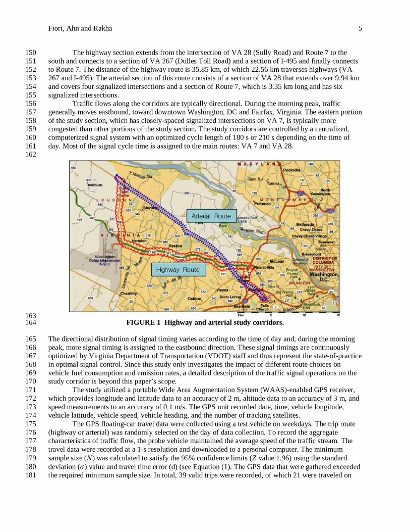
To identify the energy consumption impacts of route choice behavior, morning commute GPS data were 142 collected in the Northern Virginia area. As shown in Figure 1, the arterial route, VA Route 7, extends 143 over 22.6 km (17.25 mi) and covers 32 signalized intersections. The study section started at the 144 intersection of VA 28 (Sully Road) to the west and extended to the intersection of I-66 to the east. The 145 corridor’s entire length is divided, with a four-lane cross-section on the eastern side and a six-lane cross-146 section on the western side. The posted speed limits range from 56 km/h (35 mi/h) on the congested east 147 side to 88 km/h (55 mi/h) on the west side. The highway route connects two highway sections and two 148 arterial sections as shown in Figure 1. 149

Fiori, Ahn and Rakha 5

The highway section extends from the intersection of VA 28 (Sully Road) and Route 7 to the 150 south and connects to a section of VA 267 (Dulles Toll Road) and a section of I-495 and finally connects 151 to Route 7. The distance of the highway route is 35.85 km, of which 22.56 km traverses highways (VA 152 267 and I-495). The arterial section of this route consists of a section of VA 28 that extends over 9.94 km 153 and covers four signalized intersections and a section of Route 7, which is 3.35 km long and has six 154 signalized intersections. 155

Traffic flows along the corridors are typically directional. During the morning peak, traffic 156 generally moves eastbound, toward downtown Washington, DC and Fairfax, Virginia. The eastern portion 157 of the study section, which has closely-spaced signalized intersections on VA 7, is typically more 158 congested than other portions of the study section. The study corridors are controlled by a centralized, 159 computerized signal system with an optimized cycle length of 180 s or 210 s depending on the time of 160 day. Most of the signal cycle time is assigned to the main routes: VA 7 and VA 28. 161 162

163 FIGURE 1 Highway and arterial study corridors. 164

The directional distribution of signal timing varies according to the time of day and, during the morning 165 peak, more signal timing is assigned to the eastbound direction. These signal timings are continuously 166 optimized by Virginia Department of Transportation (VDOT) staff and thus represent the state-of-practice 167 in optimal signal control. Since this study only investigates the impact of different route choices on 168 vehicle fuel consumption and emission rates, a detailed description of the traffic signal operations on the 169 study corridor is beyond this paper’s scope. 170

The study utilized a portable Wide Area Augmentation System (WAAS)-enabled GPS receiver, 171 which provides longitude and latitude data to an accuracy of 2 m, altitude data to an accuracy of 3 m, and 172 speed measurements to an accuracy of 0.1 m/s. The GPS unit recorded date, time, vehicle longitude, 173 vehicle latitude, vehicle speed, vehicle heading, and the number of tracking satellites. 174

The GPS floating-car travel data were collected using a test vehicle on weekdays. The trip route 175 (highway or arterial) was randomly selected on the day of data collection. To record the aggregate 176 characteristics of traffic flow, the probe vehicle maintained the average speed of the traffic stream. The 177 travel data were recorded at a 1-s resolution and downloaded to a personal computer. The minimum 178 sample size (𝑁𝑁) was calculated to satisfy the 95% confidence limits (𝑍𝑍 value 1.96) using the standard 179 deviation (𝜎𝜎) value and travel time error (d) (see Equation (1). The GPS data that were gathered exceeded 180 the required minimum sample size. In total, 39 valid trips were recorded, of which 21 were traveled on 181

Fiori, Ahn and Rakha 6

the highway route and 18 were traveled on the arterial route. Ten trips on the highway route and 11 trips 182 on the arterial route were required to satisfy the minimum sample size considering a 95% confidence limit. 183

𝑁𝑁 = �1.96𝛿𝛿�2

𝜎𝜎2 (1)

While both morning and evening commute data were gathered, only morning commute data were 184 used for the analysis. A MATLAB code was developed to extract the study section data from the entire 185 morning commute travel data. The software automatically identified the first and last GPS points within 186 the study corridor using the coordinates of the boundary study sections. Following the data reduction, a 187 unique trip number was assigned to each trip. 188

ENERGY CONSUMPTION MODEL 189

The study utilized microscopic energy/fuel consumption models to identify the impact of routing options 190 on BEVs and ICEVs. The following sections briefly describe each model and how the models were 191 utilized in this study. 192

BEV Energy Model 193

The Virginia Tech Comprehensive Power-based EV Energy consumption Model (VT-CPEM) is a quasi-194 steady backward highly-resolved power-based model. The model uses instantaneous speed, acceleration, 195 and grade information as input variables. The outputs of the model are the energy consumption (EC) 196 (kWh/km), the instantaneous power consumed (kW), and the final level of the state of charge (SOC) of 197 the electric battery (%). A Nissan Leaf was utilized for the study. 198

The power at the electric motor ( 𝑃𝑃𝐸𝐸𝐸𝐸𝐸𝐸𝐸𝐸𝐸𝐸𝐸𝐸𝐸𝐸𝐸𝐸 𝑚𝑚𝑚𝑚𝐸𝐸𝑚𝑚𝐸𝐸(𝑡𝑡)) is computed, given the power at the wheels, 199 considering the driveline efficiency 𝜂𝜂𝐷𝐷𝐸𝐸𝐸𝐸𝐷𝐷𝐸𝐸𝐸𝐸𝐸𝐸𝐷𝐷𝐸𝐸 = 92% (13) and assuming that the efficiency of the electric 200 motor is 𝜂𝜂𝐸𝐸𝐸𝐸𝐸𝐸𝐸𝐸𝐸𝐸𝐸𝐸𝐸𝐸𝐸𝐸 𝑀𝑀𝑚𝑚𝐸𝐸𝑚𝑚𝐸𝐸 = 91%. This is a reasonable assumption according to SAE standards (14), and, in 201 fact, the efficiency of the electric motor of the Nissan Leaf is between 85% and 95%. Also, in this range, 202 91% is the value that minimizes the average error between the real and the estimated consumption values. 203

While the vehicle is in traction mode, energy flows from the motor to the wheels. In this case the 204 power at the electric motor is higher than the power at the wheels and the power at the wheels is assumed 205 to be positive. Alternatively, in the regenerative braking mode, energy flows from the wheels to the 206 motor. The power at the electric motor is lower than the power at the wheels and the power is assumed to 207 be negative. 208

While decelerating, the electric power is negative and the regenerative braking energy efficiency 209 (𝜂𝜂𝑅𝑅𝑅𝑅) is computed when 𝑃𝑃𝐸𝐸𝐸𝐸𝐸𝐸𝐸𝐸𝐸𝐸𝐸𝐸𝐸𝐸𝐸𝐸 𝑚𝑚𝑚𝑚𝐸𝐸𝑚𝑚𝐸𝐸(𝑡𝑡) < 0 using Equation (2). 210

𝑃𝑃𝐸𝐸𝐸𝐸𝐸𝐸𝐸𝐸𝐸𝐸𝐸𝐸𝐸𝐸𝐸𝐸 𝑚𝑚𝑚𝑚𝐸𝐸𝑚𝑚𝐸𝐸(𝑡𝑡) < 0 → 𝑃𝑃𝐸𝐸𝐸𝐸𝐸𝐸𝐸𝐸𝐸𝐸𝐸𝐸𝐸𝐸𝐸𝐸 𝑚𝑚𝑚𝑚𝐸𝐸𝑚𝑚𝐸𝐸(𝑡𝑡) = 𝑃𝑃𝐸𝐸𝐸𝐸𝐸𝐸𝐸𝐸𝐸𝐸𝐸𝐸𝐸𝐸𝐸𝐸 𝑚𝑚𝑚𝑚𝐸𝐸𝑚𝑚𝐸𝐸(𝑡𝑡) ∙ 𝜂𝜂𝑅𝑅𝑅𝑅(𝑡𝑡) (2)

The final SOC (%) is computed using Equation (3). 211

𝑆𝑆𝑆𝑆𝐶𝐶𝐹𝐹𝐸𝐸𝐷𝐷𝐹𝐹𝐸𝐸(𝑡𝑡) = 𝑆𝑆𝑆𝑆𝐶𝐶0 −�∆𝑆𝑆𝑆𝑆𝐶𝐶(𝐸𝐸)(𝑡𝑡)𝑁𝑁

𝐸𝐸=1

(3)

∆𝑆𝑆𝑆𝑆𝐶𝐶(𝐸𝐸)(𝑡𝑡)

= 𝑆𝑆𝑆𝑆𝐶𝐶(𝐸𝐸−1)(𝑡𝑡) − 𝑃𝑃𝐸𝐸𝐸𝐸𝐸𝐸𝐸𝐸𝐸𝐸𝐸𝐸𝐸𝐸𝐸𝐸 𝑚𝑚𝑚𝑚𝐸𝐸𝑚𝑚𝐸𝐸_𝐷𝐷𝐸𝐸𝐸𝐸(𝑖𝑖)

(𝑡𝑡)

3600 ∙ CapacityBattery

(4)

Here 𝑃𝑃𝐸𝐸𝐸𝐸𝐸𝐸𝐸𝐸𝐸𝐸𝐸𝐸𝐸𝐸𝐸𝐸 𝑚𝑚𝑚𝑚𝐸𝐸𝑚𝑚𝐸𝐸_𝐷𝐷𝐸𝐸𝐸𝐸(𝑖𝑖)(𝑡𝑡) is the electric power consumed considering a battery value of 212

𝜂𝜂𝑅𝑅𝐹𝐹𝐸𝐸𝐸𝐸𝐸𝐸𝐸𝐸𝐵𝐵 = 90% (15). In addition, the power consumed by the auxiliary systems (𝑃𝑃𝐴𝐴𝐴𝐴𝐴𝐴𝐸𝐸𝐸𝐸𝐸𝐸𝐹𝐹𝐸𝐸𝐵𝐵= 700 [W]) 213 (16) is considered. CapacityBattery is the capacity of the battery in (Wh). The operation range of SOC is 214

Fiori, Ahn and Rakha 7

between 20% and 95% to guarantee the safety of the battery system (17); the initial SOC is assumed to be 215 𝑆𝑆𝑆𝑆𝐶𝐶0 = 95%. 216

Given the SOC, it is possible to compute the energy consumption (EC) in (kWh/km) using 217 Equation (5). 218

𝐸𝐸𝐶𝐶 �𝑘𝑘𝑘𝑘ℎ𝑘𝑘𝑘𝑘

�

=1

3600000∙ � 𝑃𝑃𝐸𝐸𝐸𝐸𝐸𝐸𝐸𝐸𝐸𝐸𝐸𝐸𝐸𝐸𝐸𝐸 𝑚𝑚𝑚𝑚𝐸𝐸𝑚𝑚𝐸𝐸𝑛𝑛𝑛𝑛𝑛𝑛(𝑡𝑡) 𝑑𝑑𝑡𝑡

𝐸𝐸

𝑚𝑚∙

1𝑑𝑑

(5)

Here 𝑑𝑑 is the distance in (km). The parameters related to the specific electric vehicle used are 219 reported in (12) where all the characteristics of the electric vehicle used are shown. 220

The VT-CPEM model was validated against experimental data collected by the Joint Research 221 Centre (JRC) (10) of the European Commission and by the Idaho National Laboratory (INL) (11) of the 222 United States Department of Energy (U.S. DOE), and accurately estimates the energy consumption, 223 producing an average error of 5.9% relative to empirical data. More details about the VT-CPEM model 224 are reported in (1). 225

ICEV Fuel Consumption Model 226

The VT-Micro model was utilized to estimate the vehicle fuel consumption level for ICEVs using the 227 second-by-second speed profiles derived from field collected GPS data and simulation runs. The VT-228 Micro model is a mathematical model that estimates vehicle fuel consumption and emission levels for 229 individual and/or composite vehicles using instantaneous speed and acceleration as explanatory variables. 230 The VT-Micro model was developed as a regression model from experimentation with numerous 231 polynomial combinations of speed and acceleration levels to construct a dual-regime model of the form. 232

The model utilizes a number of data sources, including data collected at the Oak Ridge National 233 Laboratory (ORNL) (nine vehicles) and the Environmental Protection Agency (EPA) (101 vehicles). In 234 this study, ORNL vehicles and EPA light duty vehicles type 2 (LDV2) were utilized for the analysis. The 235 VT-Micro model fuel consumption and emission rates were found to be highly accurate compared to the 236 original data with coefficients of determination (R2) ranging from 0.92 to 0.99. The model is easy to use 237 for the evaluation of the environmental impacts of operational-level projects, including ITS. A more 238 detailed description of the model derivation is provided in the literature (20-22). 239

RESULTS 240

This section reports impacts of route selection on the energy/fuel consumption of BEVs and ICEVs. The 241 study evaluated the route choice impact using individual vehicle trips and vehicle trajectory data from a 242 microscopic traffic simulation model. 243

Field Data Analysis 244

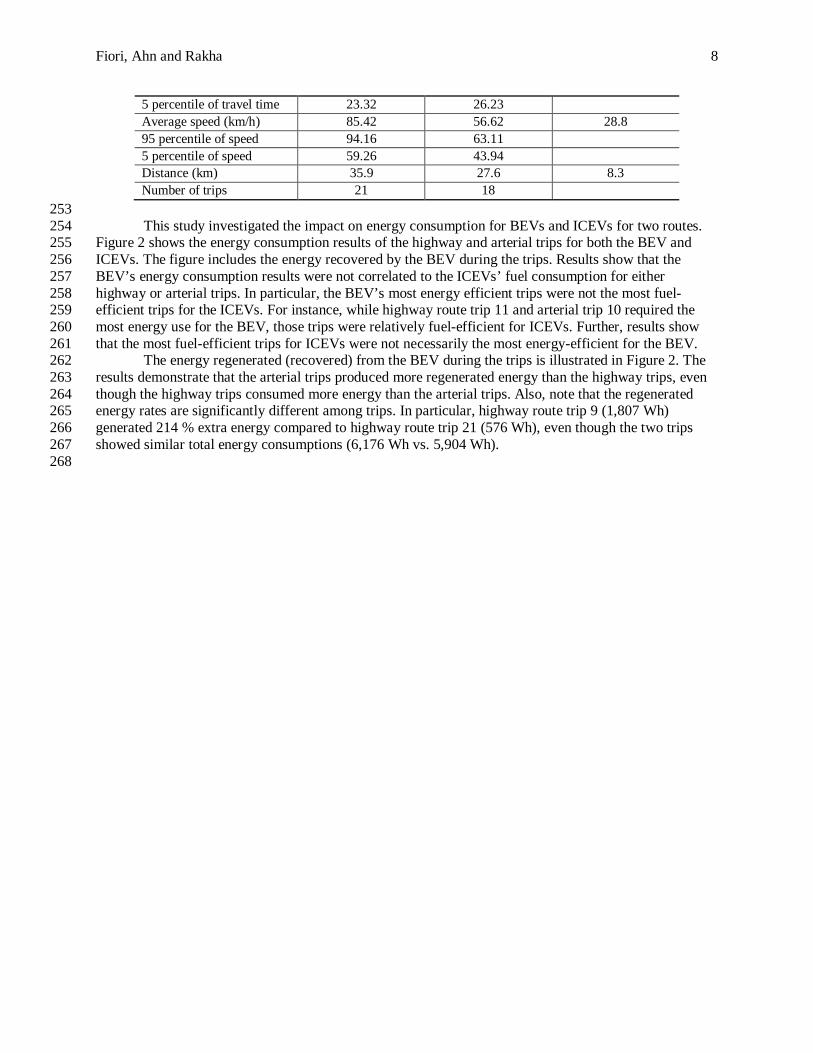
In total, 39 valid trips were analyzed—21 were highway route trips and 18 were arterial route trips. The 245 collected GPS data demonstrates that the highway trips reduced travel time by 4.27 minutes compared to 246 the arterial trips, even though the highway trips were 30% longer (35.9 km versus 27.6 km). Table 1 also 247 demonstrates that the highway trips had a significantly higher average speed (85.42 km/h) than the arterial 248 trips (56.62 km/h). Since drivers typically use routes that minimize their travel time, it is logical that 249 drivers selected the highway route in this case. 250 251 TABLE 1 Field Trip Data Characteristics 252

Highway Arterial Difference Average travel time (min) 25.63 29.9 -4.27 95 percentile of travel time 36.25 37.86

Fiori, Ahn and Rakha 8

5 percentile of travel time 23.32 26.23 Average speed (km/h) 85.42 56.62 28.8 95 percentile of speed 94.16 63.11 5 percentile of speed 59.26 43.94 Distance (km) 35.9 27.6 8.3 Number of trips 21 18 253 This study investigated the impact on energy consumption for BEVs and ICEVs for two routes. 254

Figure 2 shows the energy consumption results of the highway and arterial trips for both the BEV and 255 ICEVs. The figure includes the energy recovered by the BEV during the trips. Results show that the 256 BEV’s energy consumption results were not correlated to the ICEVs’ fuel consumption for either 257 highway or arterial trips. In particular, the BEV’s most energy efficient trips were not the most fuel-258 efficient trips for the ICEVs. For instance, while highway route trip 11 and arterial trip 10 required the 259 most energy use for the BEV, those trips were relatively fuel-efficient for ICEVs. Further, results show 260 that the most fuel-efficient trips for ICEVs were not necessarily the most energy-efficient for the BEV. 261

The energy regenerated (recovered) from the BEV during the trips is illustrated in Figure 2. The 262 results demonstrate that the arterial trips produced more regenerated energy than the highway trips, even 263 though the highway trips consumed more energy than the arterial trips. Also, note that the regenerated 264 energy rates are significantly different among trips. In particular, highway route trip 9 (1,807 Wh) 265 generated 214 % extra energy compared to highway route trip 21 (576 Wh), even though the two trips 266 showed similar total energy consumptions (6,176 Wh vs. 5,904 Wh). 267 268

Fiori, Ahn and Rakha 9

269 270

271 (a) Highway trips 272

273 (b) Arterial trips 274

FIGURE 2 Energy and fuel consumption results on highway and arterial routes. 275 276

Figure 3 compares the average energy/fuel consumption for the highway and arterial trips. For 277 this specific case study, Figure 3 demonstrates that the BEV’s energy consumption can be reduced by 278 48% if motorists use the arterial instead of the highway route. Further, the results show that regenerated 279 energy, which is typically generated during stop and go traffic conditions, was increased by 20% when 280 using the arterial route. Results also indicate that the BEV regenerated 14.8% and 26.2% of the total 281 energy consumption for the highway and arterial trips, respectively. For this specific case study, an 282 average lower speed and more regenerated energy, caused by more frequent braking actions, reduced the 283 energy consumption for the arterial trips. 284

Fiori, Ahn and Rakha 10

Figure 3 also shows an ICEV driver can save 21.6% in fuel costs on average by using the arterial 285 route. The results demonstrate that when motorists sacrifice 4.3 minutes (17%) of travel time, energy/fuel 286 efficiency is significantly improved for both BEVs and ICEVs. 287 288

289 FIGURE 3 Energy consumption on highway and arterial routes. 290

291

Simulation Results 292

This section investigates the network-wide impacts of routing choices on BEVs’ energy consumption. A 293 microscopic traffic simulation model, INTEGRATION, was utilized for the analysis. A simple network 294 was constructed to identify the energy consumption impacts of BEVs. The OD (origin-destination) 295 demand is 2,000 vehicles per hour (veh/h), and there are two routes available. The network, as illustrated 296 in Figure 4, consists of a highway route and an arterial route between an origin and a destination. A total 297 of 2,000 trips were simulated for one hour and the simulation was continued for two hours to complete all 298 2,000 trips. 299

The highway route is 5 km long with two lanes for the first 3 km section, one lane for the next 1 300 km section, and two lanes for the last 1 km section. It has a capacity of 1,800 veh/h/lane and the jam 301 density is set to 100 veh/km. The first 3 km and the last 1 km sections have a free-flow speed of 88 km/h 302 (55 mph) and the middle 1 km section has a 72 km/h free-flow speed. The arterial route is a 4 km long 303 section that has three signalized intersections located every 1 km and has an identical jam density and 304 lane capacity as the highway route. The three signals on the arterial route have a 60-second cycle length 305 with a 0.5 g/C ratio (effective green time to cycle length ratio), and are partially coordinated. 306

307

308

Fiori, Ahn and Rakha 11

FIGURE 4 Sample simulation network 309 310 Six traffic assignment scenarios were utilized in this case study. Figure 5 shows the traffic 311

assignment scenarios simulated using the INTEGRATION software. The vehicles assigned to the arterial 312 route were increased from 250 vehicles (scenario 1) to 1,500 vehicles (scenario 6) in increments of 250 313 vehicles; for example, scenario 3 shows that 750 vehicles were assigned to the arterial route and 1,250 314 vehicles were assigned to the highway route. In total, 2,000 vehicles were utilized in each scenario. 315

316

317 FIGURE 5 Traffic demand on the test network. 318

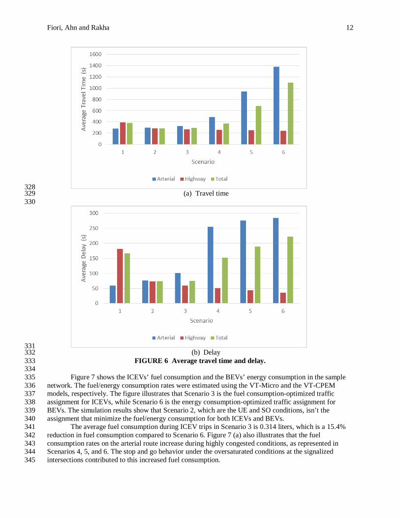
319 Figure 6 illustrates average travel time and delay results for the six traffic assignment scenarios. 320

The results show that the SO condition is achieved in scenario 2, which has the smallest total travel time 321 of the entire network. In this case study, the UE condition is also attained in scenario 2, which has a 322 similar average travel time for the two routes. The travel times of the average highway and arterial routes 323 are 299 s and 285 s, respectively. The study demonstrates that total delays are significantly increased as 324 1,000 veh/h or more are assigned to the arterial route due to the over-saturated delay at signalized 325 intersections. 326

327

Fiori, Ahn and Rakha 12

328 (a) Travel time 329

330

331 (b) Delay 332

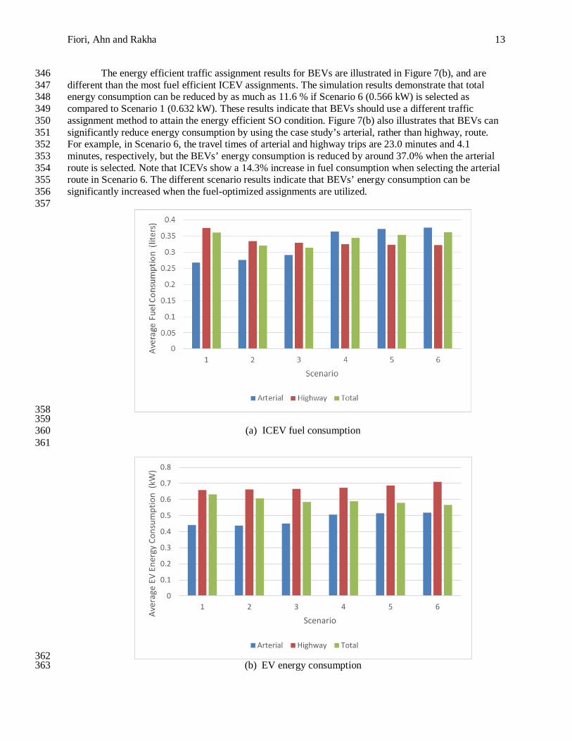
FIGURE 6 Average travel time and delay. 333 334 Figure 7 shows the ICEVs’ fuel consumption and the BEVs’ energy consumption in the sample 335

network. The fuel/energy consumption rates were estimated using the VT-Micro and the VT-CPEM 336 models, respectively. The figure illustrates that Scenario 3 is the fuel consumption-optimized traffic 337 assignment for ICEVs, while Scenario 6 is the energy consumption-optimized traffic assignment for 338 BEVs. The simulation results show that Scenario 2, which are the UE and SO conditions, isn’t the 339 assignment that minimize the fuel/energy consumption for both ICEVs and BEVs. 340

The average fuel consumption during ICEV trips in Scenario 3 is 0.314 liters, which is a 15.4% 341 reduction in fuel consumption compared to Scenario 6. Figure 7 (a) also illustrates that the fuel 342 consumption rates on the arterial route increase during highly congested conditions, as represented in 343 Scenarios 4, 5, and 6. The stop and go behavior under the oversaturated conditions at the signalized 344 intersections contributed to this increased fuel consumption. 345

Fiori, Ahn and Rakha 13

The energy efficient traffic assignment results for BEVs are illustrated in Figure 7(b), and are 346 different than the most fuel efficient ICEV assignments. The simulation results demonstrate that total 347 energy consumption can be reduced by as much as 11.6 % if Scenario 6 (0.566 kW) is selected as 348 compared to Scenario 1 (0.632 kW). These results indicate that BEVs should use a different traffic 349 assignment method to attain the energy efficient SO condition. Figure 7(b) also illustrates that BEVs can 350 significantly reduce energy consumption by using the case study’s arterial, rather than highway, route. 351 For example, in Scenario 6, the travel times of arterial and highway trips are 23.0 minutes and 4.1 352 minutes, respectively, but the BEVs’ energy consumption is reduced by around 37.0% when the arterial 353 route is selected. Note that ICEVs show a 14.3% increase in fuel consumption when selecting the arterial 354 route in Scenario 6. The different scenario results indicate that BEVs’ energy consumption can be 355 significantly increased when the fuel-optimized assignments are utilized. 356

357

358 359

(a) ICEV fuel consumption 360 361

362 (b) EV energy consumption 363

0

0.1

0.2

0.3

0.4

0.5

0.6

0.7

0.8

1 2 3 4 5 6

Aver

age

EV E

nerg

y Co

nsum

ptio

n (k

W)

Scenario

Arterial Highway Total

Fiori, Ahn and Rakha 14

FIGURE 7 Fuel consumption of ICEVs and energy consumption of BEVs. 364 365

366 FIGURE 8 Regenerated energy of BEVs. 367

368 Figure 8 highlights the BEVs’ average regenerated energy during the arterial and highway trips. 369

The results show that each scenario produces different regenerated energy rates, as the regenerated energy 370 is greatly affected by facility types and congestion levels in the case study. In general, the regenerated 371 energy is increased with the increased level of traffic delay. The maximum regenerated energy is 372 observed in Scenario 6 when the congestion level is the highest. Also, the arterial trips of Scenario 6 373 produce an extra 106% of regenerated energy compared to Scenario 1. This indicates that the regenerated 374 energy is maximized in highly congested traffic conditions and that BEVs’ energy efficient route 375 assignment can be influenced by the amount of potential regenerated energy. 376

CONCLUSIONS 377 This study investigated the impacts of route choice on energy consumption in BEVs using second-by-378 second GPS commute data and a micro-simulation study. VT-CPEM and VT-Micro models were utilized 379 to estimate the energy/fuel consumption rates of BEVs and ICEVs, respectively. The results of the case 380 studies indicate that a UE and SO traffic assignment does not necessarily minimize BEVs’ energy 381 consumption. Furthermore, the study found that the use of a faster route could actually increase BEVs’ 382 energy consumption. In addition, significant energy consumption savings (48% reduction) were observed 383 when BEV motorists utilized the arterial route, sacrificing 4.3 minutes (17%) of travel time. Results of 384 case studies lead to the conclusion that BEVs and ICEVs have different fuel/energy-optimized assignment 385 conditions, and that different energy-optimized assignments should therefore be recommended for 386 different vehicle types. Results of this traffic assignment simulation study also show that minimum BEV 387 energy consumption is achieved when most of the vehicles are assigned to the congested and low-speed 388 arterial route. Furthermore, BEVs’ energy consumption can be significantly increased when the fuel 389 optimized assignment methods are utilized and, as such, new traffic assignment methods should be 390 proposed to attain the most energy efficient BEV SO condition. 391

Finally, this study identified the impacts of regenerated power during various traffic assignment 392 scenarios. One of the main advantages of EVs is the possibility of recovering energy while braking using 393 a regenerative braking system. Study results showed that regenerated energy was greatly affected by 394 facility types and congestion levels and the most energy efficient route assignment for BEVs could be 395 significantly affected by the regenerated energy. 396

397

Fiori, Ahn and Rakha 15

ACKNOWLEDGEMENTS 398

This research effort was funded by the TranLIVE University Transportation Center. In addition, this 399 research was partially carried out in the frame of Programme STAR, financially supported by UniNA and 400 Compagnia di San Paolo. 401

REFERENCES 402

1. Fiori, C., K. Ahn, and H.A. Rakha. Power-based electric vehicle energy consumption model: 403 Model development and validation. Applied Energy, Vol. 168, 2016, pp. 257-268. 404

2. Knowles, M., H. Scott, and D. Baglee. The effect of driving style on electric vehicle performance, 405 economy and perception. International Journal of Electric and Hybrid Vehicles, Vol. 4, No. 3, 406 2012, pp. 228-247. 407

3. Richter, M., S. Zinser, and H. Kabza. Comparison of eco and time efficient routing of ICEVs, 408 BEVs and PHEVs in inner city traffic. In Vehicle Power and Propulsion Conference (VPPC), 409 2012 IEEE, IEEE, 2012, pp. 1165-1169. 410

4. Liu, C., J. Wu, and C. Long. Joint Charging and Routing Optimization for Electric Vehicle 411 Navigation Systems. In International Federation of Automatic Control, 2014. 412

5. Artmeier, A., J. Haselmayr, M. Leucker, and M. Sachenbacher. The optimal routing problem in 413 the context of battery-powered electric vehicles. In Workshop CROCS at CPAIOR-10, 2nd 414 International Workshop on Constraint Reasoning and Optimization for Computational 415 Sustainability, 2010. 416

6. Sachenbacher, M., M. Leucker, A. Artmeier, and J. Haselmayr.. Efficient Energy-Optimal 417 Routing for Electric Vehicles. In AAAI, 2011. 418

7. Bhavsar, P., M. Chowdhury, Y. He, and M. Rahman. A network wide simulation strategy of 419 alternative fuel vehicles. Transportation Research Part C: Emerging Technologies, Vol. 40, 420 2014, pp. 201-214. 421

8. Bingham, C., C. Walsh, and S. Carroll. Impact of driving characteristics on electric vehicle 422 energy consumption and range. Intelligent Transport Systems, IET, Vol. 6, No. 1., 2012, pp. 29-423 35. 424

9. Sivak, M. and B. Schoettle. Eco-driving: Strategic, tactical, and operational decisions of the 425 driver that influence vehicle fuel economy. Transport Policy, Vol. 22, 2012. pp. 96-99. 426

10. De Gennaro, M., Paffumi, E., Martini, G., Manfredi, U. et al. Experimental Test Campaign on a 427 Battery Electric Vehicle: Laboratory Test Results (Part 1). SAE International Journal of 428 Alternative Powertrains. Vol. 4, No. 1, 2015, pp. 100-114. 429

11. U.S. Department of Energy (DOE). Advanced Vehicle Testing Activity (AVTA) of the Idaho 430 Nation Laboratory (INL), 2013. http://avt.inel.gov/pdf/fsev/fact2013nissanleaf.pdf. Accessed 431 June 30, 2015. 432

12. Nissan. Nissan Leaf Characteristiscs, 2015. http://www.nissanusa.com/electric-cars/leaf/. 433 Accessed June 30, 2015. 434

13. Rakha, H.A., K. Ahn, K. Moran, B. Saerens, and E. Van den Bulck.Virginia tech comprehensive 435 power-based fuel consumption model: model development and testing. Transportation Research 436 Part D: Transport and Environment, Vol. 16, No. 7, 2011, pp. 492-503. 437

14. SAE International. 2011 Nissan Leaf Vehicle Overview. 438 http://c.ymcdn.com/sites/www.electricauto.org/resource/resmgr/media/nissan_leaf_sae_2_11.pdf. 439 Accessed July 14, 2015. 440

15. Rydh, C.J. and B.A. Sandén. Energy analysis of batteries in photovoltaic systems. Part I: 441 Performance and energy requirements. Energy Conversion and Management, Vol. 46, No. 11, 442 2005, pp. 1957-1979. 443

Fiori, Ahn and Rakha 16

16. Szadkowski, B., P.J. Chrzan, and D. Roye. A study of energy requirements for electric and hybrid 444 vehicles in cities. n Proceedings of the 2003 International Conference on Clean, Efficient and 445 Safe Urban Transport, 2003, pp. 4-6. 446

17. Joos, G., M. De Freige, and M. Dubois. Design and simulation of a fast charging station for 447 phev/ev batteries. In Electric Power and Energy Conference (EPEC), 2010 IEEE, August 2010, 448 pp. 1-5. 449

18. Gao, Y., L. Chu, and M. Ehsani. Design and control principles of hybrid braking system for EV, 450 HEV and FCV. In Vehicle Power and Propulsion Conference, 2007, VPPC 2007, IEEE. 9-12 451 September, 2007, pp. 384-391. 452

19. Donovan, John. Chevy Volt Tech Watch: Regenerative Braking. Design News, November, 453 2011.http://www.designnews.com/document.asp?doc_id=235313. Accessed June 30, 2015. 454

20. Ahn, K., H. Rakha, A. Trani, and M. Van Aerde. Estimating vehicle fuel consumption and 455 emissions based on instantaneous speed and acceleration levels. Journal of Transportation 456 Engineering, Vol. 128, No. 2, 2002. pp. 182-190. 457

21. Ahn, K., H. Rakha, and A. Trani. Microframework for modeling of high-emitting vehicles. In 458 Transportation Research Record: Journal of the Transportation Research Board, No. 1880, 459 Transportation Research Board of the National Academies, Washington, D.C., 2004, pp. 39-49. 460

22. Rakha, H., K. Ahn, and A. Trani. Development of VT-Micro model for estimating hot stabilized 461 light duty vehicle and truck emissions. Transportation Research Part D-Transport and 462 Environment, Vol. 9, No. 1, 2004, pp. 49-74. 463

23. Becker, T.A., I. Sidhu, and B. Tenderich, Electric vehicles in the United States: a new model with 464 forecasts to 2030. (Technical Brief No. 2009.1.v.2.0). Center for Entrepreneurship & Technology, 465 University of California, Berkeley, Berkeley, California, 2009. 466

467