arX

iv:1

601.

0587

5v4

[cs.

IT]

20 N

ov 2

016

1

Distributed Simulation of Continuous RandomVariables

Cheuk Ting Li and Abbas El GamalDepartment of Electrical Engineering, Stanford University

Email: ctli@stanford.edu, abbas@ee.stanford.edu

Abstract

We establish the first known upper bound on the exact and Wyner’s common information ofn continuous random variablesin terms of the dual total correlation between them (which isa generalization of mutual information). In particular, weshowthat when the pdf of the random variables is log-concave, there is a constant gap ofn2 log e + 9n log n between this upperbound and the dual total correlation lower bound that does not depend on the distribution. The upper bound is obtained using acomputationally efficient dyadic decomposition scheme forconstructing a discrete common randomness variableW from whichthen random variables can be simulated in a distributed manner. We then bound the entropy ofW using a new measure, whichwe refer to as the erosion entropy.

Index Terms

Exact common information, Wyner’s common information, log-concave distribution, dual total correlation, channel synthesis.

I. I NTRODUCTION

This paper is motivated by the following question. Alice would like to simulate a random variableX1 and Bob wouldlike to simulate another random variableX2 such that(X1, X2) are jointly Gaussian with a prescribed mean and covariancematrix. Can these two random variables be simulated in a distributed manner with only a finite amount of common randomnessbetween Alice and Bob?

We answer this question in the affirmative forn continuous random variables under certain conditions on their joint pdf,including when it is log-concave such as Gaussian.

The general distributed randomness generation setup we consider is depicted in Figure 1. There aren agents (e.g., processorsin a computer cluster or nodes in a communication network) that have access tocommon randomnessW ∈ {0, 1}∗. Agenti ∈ [1 : n] wishes to simulate the random variableXi usingW and its local randomness, which is independent ofW andthe local randomness at other agents, such thatXn = (X1, . . . , Xn) follows a prescribed distributionexactly. The distributedrandomness simulation problem is to find the common randomnessW ∗ with the minimum average description lengthR∗,referred to in [1] as theexact common informationbetweenXn, and the scheme that achieves this exact common information.

SinceW can be represented by an optimal prefix-free code, e.g., a Huffman code or the code in [2] if the alphabet is infinite,the average description lengthR∗ can be upper bounded asH(W ) ≤ R∗ < H(W ) + 1, whereW minimizesH(W ). Hencein this paper we will focus on investigatingW that minimizesH(W ) instead ofR∗.

The above setting was introduced in [1] for two discrete random variables and the minimum entropy ofW , referred to asthe common entropy, is given by

G(X1;X2) = minW :X1⊥⊥X2|W

H(W ). (1)

A similar quantity for channel simulation was also studied by Harsha et. al. [3]. ComputingG(X1;X2), even for moderate sizerandom variable alphabets, can be computationally difficult since it involves minimizing a concave function over a non-convexset; see [1] for some cases whereG can be computed and for some properties that can be exploitedto compute it. Hence themain difficulty in constructing a scheme that achievesG (within 1-bit) for a given(X1, X2) distribution is finding the optimalcommon randomnessW that achieves it.

It can be readily shown that

I(X1;X2) ≤ J(X1;X2) ≤ G(X1;X2) ≤ min{H(X1), H(X2)}, (2)

whereJ(X1;X2) = min

W :X1⊥⊥X2|WI(W ;X1, X2) (3)

The work of C. T. Li was partially supported by a Hong Kong Alumni Stanford Graduate Fellowship. This paper was presented in part at the IEEEInternational Symposium on Information Theory, Barcelona, July 2016.

2

W ∈ {0, 1}∗

Common RandomnessSource

Agent 1 Agent 2 Agentn

X1 X2 Xn

Figure 1. Distributed randomness generation setting. Common randomnessW is broadcast ton agents and agenti ∈ [1 : n] generatesXi usingW and itlocal randomness.

is Wyner’s common information [4], which is the minimum amount of common randomness rate needed to generate the discretememoryless source (DMS)(X1, X2) with asymptotically vanishing total variation. The notionof exact common informationrate G(X1;X2), which is the minimum amount of common randomness rate needed to generate the DMS(X1, X2) exactly,was also introduced in [1]. It was shown that: (i) in generalJ ≤ G ≤ G, (ii) G can be strictly larger thanG, and (iii) insome casesG(X1;X2) = J(X1;X2). It is not known, however, ifG(X1;X2) = J(X1;X2) in general. As such, we do notconsiderG further in this paper.

The above results can be extended ton random variables. First, it is straightforward to extend the common entropy in (1)to n general random variables to obtain

G(X1; . . . ;Xn) = minW :X1⊥⊥X2⊥⊥...⊥⊥Xn|W

H(W ). (4)

Second, in [5], [6] Wyner’s common information was extendedto n discrete random variables to obtain

J(X1; . . . ;Xn) = minW :X1⊥⊥X2⊥⊥...⊥⊥Xn|W

I(W ;X1, . . . , Xn).

The operational implications of Wyner’s common information for two continuous random variables was studied in [7]. Wyner’scommon information between scalar jointly Gaussian randomvariables is computed in [7], and the result is extended to Gaussianvectors in [8], and to outputs of additive Gaussian channelsin [9].

We can also generalize the bounds in (2) ton random variables to obtain

ID(X1;X2; . . . ;Xn) ≤ J(X1;X2; . . . ;Xn) ≤ G(X1;X2; . . . ;Xn) ≤ mini

H(X1, . . . , Xi−1, Xi+1, . . . Xn), (5)

whereID is thedual total correlation[10] — a generalization of mutual information defined as

ID(X1;X2; . . . ;Xn) = H(X1, . . . , Xn)−n∑

i=1

H(Xi |X1, . . . , Xi−1, Xi+1, . . . , Xn).

Details of the derivation of the lower bound in (5) can be found in Appendix A. Note that the lower bound onJ continues tohold for continuous random variables after replacing the entropyH in the definition ofID with the differential entropyh. Thereis no corresponding upper bound to (5) for continuous randomvariables, however, and it is unclear under what conditionsGis finite.

In this paper we devise a computationally efficient scheme for constructing a common randomness variableW for distributedsimulation ofn continuous random variables and establish upper bounds on its entropy, which in turn provide upper boundson G. In particular we establish the following upper bound onG when the pdf ofXn is log-concave

ID ≤ J ≤ G ≤ ID + n2 log e+ 9n logn.

For n = 2, this bound reduces to

I(X1;X2) ≤ J(X1;X2) ≤ G(X1;X2) ≤ I(X1;X2) + 24.

Applying this result to two jointly Gaussian random variables shows that only a finite amount of common randomness isneeded for their distributed simulation. The above upper bound also provides an upper bound on Wyner’s common informationbetweenn continuous random variables with log-concave pdf. This is an interesting result since computing Wyner’s commoninformation forn continuous random variables is very difficult in general andthere is no previously known upper bound on it.

3

Our distributed randomness simulation scheme uses a dyadicdecomposition procedure to construct the common randomnessvariableW . ForXn uniformly distributed over a setA, our decomposition method partitionsA into hypercubes. The commonrandomnessW is defined as the position and size of the hypercube that contains X1, . . . , Xn represented via an optimalprefix-free code. Conditioned onW , the random variablesXn are independent and uniformly distributed over line segments,which when combined with local randomness facilitates distributed exact simulation. This scheme is extended to non-uniformlydistributedXn by performing the same dyadic decomposition on the positivepart of the hypograph of the pdf ofXn. SinceboundingH(W ) directly is quite difficult, we bound it using theerosion entropyof the set, which is a new measure that isshift invariant.

The cardinality of the random variableW needed for exact distributed simulation of continuous random variables is ingeneral infinite. By terminating the dyadic decomposition at a finite iteration, however, we show that the random variables canbe approximately simulated using a fixed length code such that for log-concave pdfs, the total variation distance between thesimulated and prescribed pdfs can be bounded as a function ofthe dual total correlation and the cardinality ofW . This resultprovides an upper bound on the one-shot version of Wyner’s common information with total variation constraint.

The rest of the paper is organized as follows. In Section II, we introduce the aforementioned dyadic decomposition schemeand establish an upper bound onG when the random variables are uniformly distributed over anorthogonally convex set. InSection III, we extend this bound to non-uniform distributions with orthogonally concave pdf and establish our main result onlog-concave pdfs. In Section IV, we establish an upper boundon the one-shot version of Wyner’s common information withtotal variation constraint. In Appendix B, we provide details on the implementation of the coding scheme for constructing thecommon randomness variable.

A. Notation

Throughout this paper, we assume thatlog is base 2 and the entropyH is in bits. We use the notation:[a : b] = [a, b] ∩ ZandX[1:n]\i = (X1, . . . , Xi−1, Xi+1, . . . , Xn).

A set A ⊆ Rn is said to beorthogonally convexif for any line L parallel to one of then axes,L ∩ A is a connected set(empty, a point, or an interval). A functionf is said to be orthogonally concave if itshypograph{(x, α) : x ∈ Rn, α ≤ f(x)}is orthogonally convex.

We denote thei-th standard basis vector ofRn by ei. We denote the volume of a Lebesgue measurable setA ⊆ Rn byVn(A) =

´

Rn 1A(x)dx. If A ⊆ B ⊆ Rn, whereB is anm-dimensional affine subspace, we denote them-dimensional volumeof A by Vm(A) =

´

B1A(x)dx.

We define the projection of a pointx ∈ Rn as

Pi1,...,ik(x) = (xi1 , . . . , xik) ∈ Rk,

and the projection of a setA ⊆ Rn onto the dimensionsi1, . . . , ik as

Pi1,...,ik(A) = {(xi1 , . . . , xik ) : x ∈ A} ⊆ Rk.

We use the shorthand notation

P\i(A) = P1,2,...,i−1,i+1,...,n(A),

VPi1,...,ik(A) = Vk(Pi1,...,ik(A)),

VP\i(A) = Vn−1(P\i(A)).

For A,B ⊆ Rn, A+B denotes the Minkowski sum{a+ b : a ∈ A, b ∈ B}, and forx ∈ Rn, A+ x = {a+ x : a ∈ A}. Forγ ∈ R, γA = {γa : a ∈ A}. For M ∈ Rn×n, MA = {Ma : a ∈ A}. The erosionof the setA by the setB is defined asA⊖B = {x ∈ Rn : B + x ⊆ A}.

For a setA ⊆ Rn where0 ∈ A, the radial functionρA : Rn → R is defined asρA(x) = sup {λ ≥ 0 : λx ∈ A}.

II. U NIFORM DISTRIBUTION OVER A SET

We first define the dyadic decomposition of a set, which is the building block of our distributed randomness simulationscheme.

Definition 1 (Dyadic decomposition). For v ∈ Zn andk ∈ Z, we define the hypercubeCk,v = 2−k([0, 1]n + v) ⊂ Rn. For asetA ⊆ Rn with a boundary of measure zero andk ∈ Z, define the set

Dk(A) ={

v ∈ Zn : Ck,v ⊆ A andCk−1,⌊v/2⌋ * A}

,

where⌊v/2⌋ is the vector formed by the entries⌊vi/2⌋.The dyadic decompositionof A is the partitioning ofA into hypercubes{Ck,v} such thatv ∈ Dk(A) and k ∈ Z. Since

every pointx in the interior ofA is contained in some hypercube inA, the interior is contained in∪k∈Z, v∈Dk(A)Ck,v , andthe set of points inA not covered by the hypercubes has measure zero.

4

For Xn ∼ Unif(A), denote byCK,V , V ∈ DK(A), the hypercube that containsXn and let thedyadic decompositionrandom variableWA = (K,V ). Then conditioned onWA = (k, v), Xn ∼ Unif(Ck,v), that is,X1, . . . , Xn are conditionallyindependent givenWA. Hence, we can use the dyadic decomposition to perform distributed randomness simulation as follows.

1) The common randomness source generatesxn according to a uniform pdf overA and findswA = (k, v) such thatv ∈ Dk(A) and xn ∈ Ck,v.

2) The common randomness source representswA by a codeword from an agreed upon optimal prefix-free code andsendsit to the processors (from this point on, we will assume thatWA is always represented by an optimal prefix-free code).

3) Upon receiving and recoveringwA = (k, v), agenti generatesXi ∼ Unif[2−kvi, 2−k(vi + 1)].

The implementation details of this scheme are provided in Appendix B.To illustrate the above dyadic decomposition scheme, consider the following.

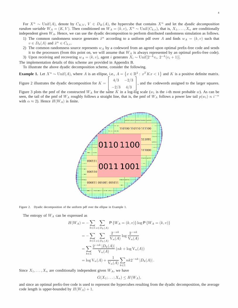
Example 1. Let Xn ∼ Unif(A), whereA is an ellipse, i.e.,A ={

x ∈ R2 : xTKx < 1}

andK is a positive definite matrix.

Figure 2 illustrates the dyadic decomposition forK =

4/3 −2/3−2/3 4/3

, and the codewords assigned to the larger squares.

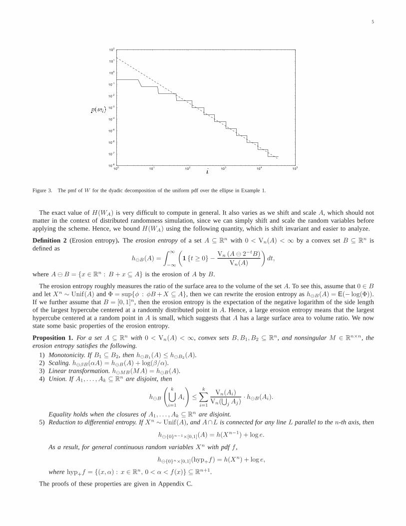
Figure 3 plots the pmf of the constructedWA for the sameK in a log-log scale (wi is the i-th most probablew). As can beseen, the tail of the pmf ofWA roughly follows a straight line, that is, the pmf ofWA follows a power law tailp(wi) ∝ i−α

with α ≈ 2). HenceH(WA) is finite.

Figure 2. Dyadic decomposition of the uniform pdf over the ellipse in Example 1.

The entropy ofWA can be expressed as

H(WA) = −∑

k∈Z

∑

v∈Dk(A)

P {WA = (k, v)} logP {WA = (k, v)}

= −∑

k∈Z

∑

v∈Dk(A)

2−nk

Vn(A)log

2−nk

Vn(A)

=∑

k∈Z

2−nk |Dk(A)|Vn(A)

(nk + logVn(A))

= logVn(A) +1

Vn(A)

∑

k∈Z

nk2−nk |Dk(A)| .

SinceX1, . . . , Xn are conditionally independent givenWA, we have

G(X1; . . . ;Xn) ≤ H(WA),

and since an optimal prefix-free code is used to represent thehypercubes resulting from the dyadic decomposition, the averagecode length is upper-bounded byH(WA) + 1.

5

100

101

102

103

104

105

10-8

10-7

10-6

10-5

10-4

10-3

10-2

10-1

100

101

102

Figure 3. The pmf ofW for the dyadic decomposition of the uniform pdf over the ellipse in Example 1.

The exact value ofH(WA) is very difficult to compute in general. It also varies as we shift and scaleA, which should notmatter in the context of distributed randomness simulation, since we can simply shift and scale the random variables beforeapplying the scheme. Hence, we boundH(WA) using the following quantity, which is shift invariant and easier to analyze.

Definition 2 (Erosion entropy). The erosion entropyof a setA ⊆ Rn with 0 < Vn(A) < ∞ by a convex setB ⊆ Rn isdefined as

h⊖B(A) =

ˆ ∞

−∞

(

1 {t ≥ 0} − Vn (A⊖ 2−tB)

Vn(A)

)

dt,

whereA⊖B = {x ∈ Rn : B + x ⊆ A} is the erosion ofA by B.

The erosion entropy roughly measures the ratio of the surface area to the volume of the setA. To see this, assume that0 ∈ Band letXn ∼ Unif(A) andΦ = sup{φ : φB+X ⊆ A}, then we can rewrite the erosion entropy ash⊖B(A) = E(− log(Φ)).If we further assume thatB = [0, 1]n, then the erosion entropy is the expectation of the negativelogarithm of the side lengthof the largest hypercube centered at a randomly distributedpoint in A. Hence, a large erosion entropy means that the largesthypercube centered at a random point inA is small, which suggests thatA has a large surface area to volume ratio. We nowstate some basic properties of the erosion entropy.

Proposition 1. For a setA ⊆ Rn with 0 < Vn(A) < ∞, convex setsB,B1, B2 ⊆ Rn, and nonsingularM ∈ Rn×n, theerosion entropy satisfies the following.

1) Monotonicity. IfB1 ⊆ B2, thenh⊖B1(A) ≤ h⊖B2(A).2) Scaling.h⊖βB(αA) = h⊖B(A) + log(β/α).3) Linear transformation.h⊖MB(MA) = h⊖B(A).4) Union. If A1, . . . , Ak ⊆ Rn are disjoint, then

h⊖B

(

k⋃

i=1

Ai

)

≤k∑

i=1

Vn(Ai)

Vn(⋃

j Aj)· h⊖B(Ai).

Equality holds when the closures ofA1, . . . , Ak ⊆ Rn are disjoint.5) Reduction to differential entropy. IfXn ∼ Unif(A), andA∩L is connected for any lineL parallel to then-th axis, then

h⊖{0}n−1×[0,1](A) = h(Xn−1) + log e.

As a result, for general continuous random variablesXn with pdf f ,

h⊖{0}n×[0,1](hyp+f) = h(Xn) + log e,

wherehyp+f = {(x, α) : x ∈ Rn, 0 < α < f(x)} ⊆ Rn+1.

The proofs of these properties are given in Appendix C.

6

In the following proposition we show thatH(WA) can be upper bounded using the erosion entropy. Moreover we show thatthe erosion entropy is the average of the dyadic decomposition entropy under random shifting and scaling.

Proposition 2. For a setA ⊆ Rn with a boundary of measure zero, we have

H(WA) ≤ logVn(A) + nh⊖[0,1]n(A) + 2n.

Moreover, for anyT ∈ Z, T > (1/n) logVn(A) + 1, whenUn ∼ Unif[0, 2T ] i.i.d., Θ ∼ Unif[0, 1] independent ofUn andΛ = 2Θ, we have

E [H(WΛA+U )] = logVn(A) + nh⊖[0,1]n(A).

The proof of this proposition is given in Appendix D.For an orthogonally convex setA, the entropy of the dyadic decomposition can be bounded by the volume ofA and the

volume of its projection as follows.

Theorem 1. Let A ⊆ Rn be an orthogonally convex set with0 < Vn(A) <∞ andXn ∼ Unif(A), then

H(WA) ≤ n log

(

n∑

i=1

VP\i(A)

)

− (n− 1) logVn(A) + (2 + log e)n.

Moreover, by applying the randomization in Proposition 2, we obtain

G(X1; · · · ;Xn) ≤ n log

(

n∑

i=1

VP\i(A)

)

− (n− 1) logVn(A) + n log e. (6)

If the setA is not orthogonally convex but can be partitioned into orthogonally convex sets, then the property of erosionentropy of union of sets in Proposition 1 can be used to boundH(WA). We now use the above theorem to upper boundGfor the uniform pdf over an ellipse example.Example 1 (continued). Applying (6) to the uniform pdf over the ellipse A =

{

x ∈ R2 : xTKx ≤ 1}

, we obtain

H(WA) ≤ 2 log

(

2∑

i=1

VP\i(A)

)

− logV2(A) + 4 + 2 log e

= 2 log

(

2

√

K11

detK+ 2

√

K22

detK

)

− log

(

π

√

1

detK

)

+ 4 + 2 log e

= log

(

π−1

(√K11 +

√K22

)2

√detK

)

+ 6 + 2 log e.

Comparing this to the mutual information for the uniform pdfover the ellipse, we have

I(X1;X2) = log

(

πe−1

√

K11K22

detK

)

.

Note that the gap betweenH(WA) and I(X1;X2) depends on the ratio between(√

K11 +√K22

)2and√K11K22, which

becomes very large whenK11 ≫ K22. For example, ifK = diag(10000, 1), then√K11K22 = 100 and I(X1;X2) ≈ 0.21.

On the other hand,(√

K11 +√K22

)2= 10201 and the bound onH(WA) is 13.02. In the next section we show that this gap

can be reduced and bounded by a constant by appropriately scaling A.

To prove Theorem 1, we need the following lemma, which boundsthe volume of the erosion ofA by a hypercube.

Lemma 1. For any orthogonally convex setA ⊆ Rn with 0 < Vn(A) <∞ and γ ≥ 0, the setA⊖(

[0, γ]× {0}n−1)

⊆ A isorthogonally convex, and

Vn

(

A⊖(

[0, γ]× {0}n−1))

≥ Vn(A)−ˆ

P[2:n](A)

min {γ , V1 (A ∩ (span(e1) + x))} dxn2 ,

wherespan(e1) + x = {(α, x2, x3, . . . , xn) : α ∈ R} ⊆ Rn. As a result,

Vn (A⊖ [0, γ]n) ≥ Vn(A) −n∑

i=1

ˆ

P\i(A)

min {γ , V1 (A ∩ (span(ei) + x))} dx[1:n]\i.

7

Proof: We first prove the following result on the erosion ofA by a line segment: for any orthogonally convex setA ⊆ Rn

with 0 < Vn(A) <∞ andγ ≥ 0, the setA⊖(

[0, γ]× {0}n−1)

⊆ A is orthogonally convex, and

Vn

(

A⊖(

[0, γ]× {0}n−1))

≥ Vn(A)−ˆ

P[2:n](A)

min {γ , V1 (A ∩ (span(e1) + x))} dx.

Note that

A⊖(

[0, γ]× {0}n−1)

= {x : x+ αe1 ∈ A for all α ∈ [0, γ]}= {x : x ∈ A− αe1 for all α ∈ [0, γ]}=

⋂

α∈[0,γ]

(A− αe1)

is the intersection of orthogonally convex sets, and therefore is orthogonally convex. Also

Vn(A)−Vn

(

A⊖(

[0, γ]× {0}n−1))

= Vn {x ∈ A : x+ αe1 /∈ A for someα ∈ [0, γ]}

=

ˆ

P[2:n](A)

V1 {x1 ∈ R : (x1, x2, . . . , xn) ∈ A, (x1 + α, x2, . . . , xn) /∈ A for someα ∈ [0, γ]}dxn2

=

ˆ

P[2:n](A)

V1 {x ∈ A ∩ (span(e1) + x) : x+ αe1 /∈ A ∩ (span(e1) + x) for someα ∈ [0, γ]} dxn2

≤ˆ

P[2:n](A)

min {γ , V1 (A ∩ (span(e1) + x))} dxn2 ,

where the last inequality follows sinceA ∩ (span(e1) + x) is connected.By repeating this result for each axis, and observing that

´

P\i(A) min {γ , V1 (A ∩ (span(ei) + x))} dx[1:n]\i cannot increasewhenA is replaced with an orthogonally convex subset ofA, we obtain the second bound.

We are now ready to prove Theorem 1.

Proof of Theorem 1:By Proposition 2, the theorem can be proved by boundingh⊖[0,1]n(A). Note that by Lemma 1,

h⊖[0,1]n(A) =

ˆ ∞

−∞

(

1 {t ≥ 0} − Vn (A⊖ [0, 2−t]n)

Vn(A)

)

dt

≤ˆ ∞

−∞

(

1 {t ≥ 0} − 1

Vn(A)max

(

0, Vn(A)−n∑

i=1

ˆ

P\i(A)

min{

2−t , V1 (A ∩ (span(ei) + x))}

dx[1:n]\i

))

dt

≤ˆ ∞

−∞

(

1 {t ≥ 0} −max

(

0, 1− 1

Vn(A)

n∑

i=1

ˆ

P\i(A)

2−tdx[1:n]\i

))

dt

=

ˆ ∞

−∞

(

1 {t ≥ 0} −max

(

0, 1− 2−t

∑ni=1 VP\i(A)

Vn(A)

))

dt

= log

(∑n

i=1 VP\i(A)

Vn(A)

)

+ log e.

For the second result, note that the randomization in Proposition 2 does not affect the right hand side of Theorem 1, whichcompletes the proof of the theorem.

A. Scaling

In this section, we present a tighter bound on the common entropy between continuous random variables by first scalingA along each dimension, that is, by performing a linear transformationDA whereD is a diagonal matrix. This correspondsto scaling the random variableXi by Dii, i ∈ [1 : n], before applying the scheme. This new bound will be in terms of thefollowing.

Definition 3 (Truncated differential entropy). Let Xn ∼ f(xn) and define its truncated differential entropyhζ(Xn) for

ζ ∈ (0, 1], as

hζ(Xn) =

ˆ

Rn

−ζ−1 min {ξ, f(x)} log(

ζ−1 min {ξ, f(x)})

dx,

whereξ > 0 such thatˆ

Rn

min {ξ, f(x)} dx = ζ.

8

And defineh0(X

n) = limζ→0

hζ(Xn) = logVn {x : f(x) > 0} .

Note thathζ(Xn) is decreasing inζ from h0(X

n) (the entropy of the uniform pdf on the support ofXn) to h1(Xn) = h(Xn).

We now state the main result of this section, which shows thatthe gap betweenH(WDA) and ID depends on how closeh1/n(X[1:n]\i) andh(X[1:n]\i), i ∈ [1 : n], are to each other.

Theorem 2. For any orthogonally convex setA ⊆ Rn with 0 < Vn(A) <∞, there exists a diagonal matrixD ∈ Rn×n withpositive diagonal entries such that the entropy of the dyadic decomposition ofDA = {Dx : x ∈ A} is bounded by

H(WDA) ≤n∑

i=1

h1/n(X[1:n]\i)− (n− 1) logVn(A) + n logn+ (2 + log e)n.

Equivalently, whenXn ∼ Unif(A),

H(WDA) ≤ ID(X1; · · · ;Xn) +n∑

i=1

(

h1/n(X[1:n]\i)− h(X[1:n]\i))

+ n logn+ (2 + log e)n.

Moreover, by applying the randomization in Proposition 2, we obtain

ID ≤ J ≤ G ≤ ID +

n∑

i=1

(

h1/n(X[1:n]\i)− h(X[1:n]\i))

+ n logn+ n log e.

The proof of this theorem and a method for finding findD are given in Appendix E.We illustrate the above bound in the following.

Example 1 (continued). Applying Theorem 2 to the uniform pdf over the ellipse A ={

x ∈ R2 : xTKx ≤ 1}

, we have

H(WDA) ≤2∑

i=1

h1/2(X[1:2]\i)− logV2(A) + 6 + 2 log e

≤2∑

i=1

log(

VP\i(A))

− logV2(A) + 6 + 2 log e

= log

(

2

√

K11

detK

)

+ log

(

2

√

K22

detK

)

− log

(

π

√

1

detK

)

+ 6 + 2 log e

= log

(

π−1

√

K11K22

detK

)

+ 8 + 2 log e.

In comparison, the mutual information is

I(X1;X2) = log

(

πe−1

√

K11K22

detK

)

,

and the gap betweenH(WDA) and I(X1;X2) is bounded by a constant. Figure 4 plots the values ofH(WDA) (calculatedby finding all squares in the dyadic decomposition with side length at least2−11, which yields a precise estimate), the upper

bound in Theorem 2, andI(X1;X2) for K = 11−t2

1 −t−t 1

, t ∈ [0, 1].

III. N ONUNIFORM DISTRIBUTIONS

In this section, we extend our results to the case in which thepdf of Xn is not necessarily uniform. LetXn ∼ f(xn) andlet the support off be A. We add a random variableZ such that(X1, . . . , Xn, Z) ∼ Unif(hyp+f), wherehyp+f is thepositive strict hypographdefined as

hyp+f = {(x, α) : x ∈ Rn, 0 < α < f(x)} ⊆ Rn+1.

Note that the marginal pdf ofXn is f . Assuming thathyp+f is orthogonally convex, i.e.,f is orthogonally concave, we canapply the results for the uniform pdf case in Section II. To illustrate this extension, consider the following.

Example 2. Let (X1, X2) be zero mean Gaussian with covariance matrixK =

1/8 1/16

1/16 1/8

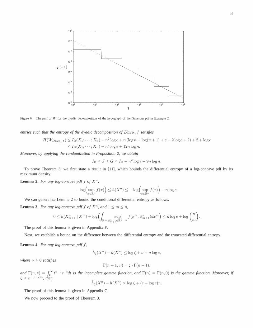
. Figure 5 plots the cubes

with side length≥ 2−3 of the dyadic decomposition of the positive strict hypograph of this pdf. Note that the cubes are scaled

9

t

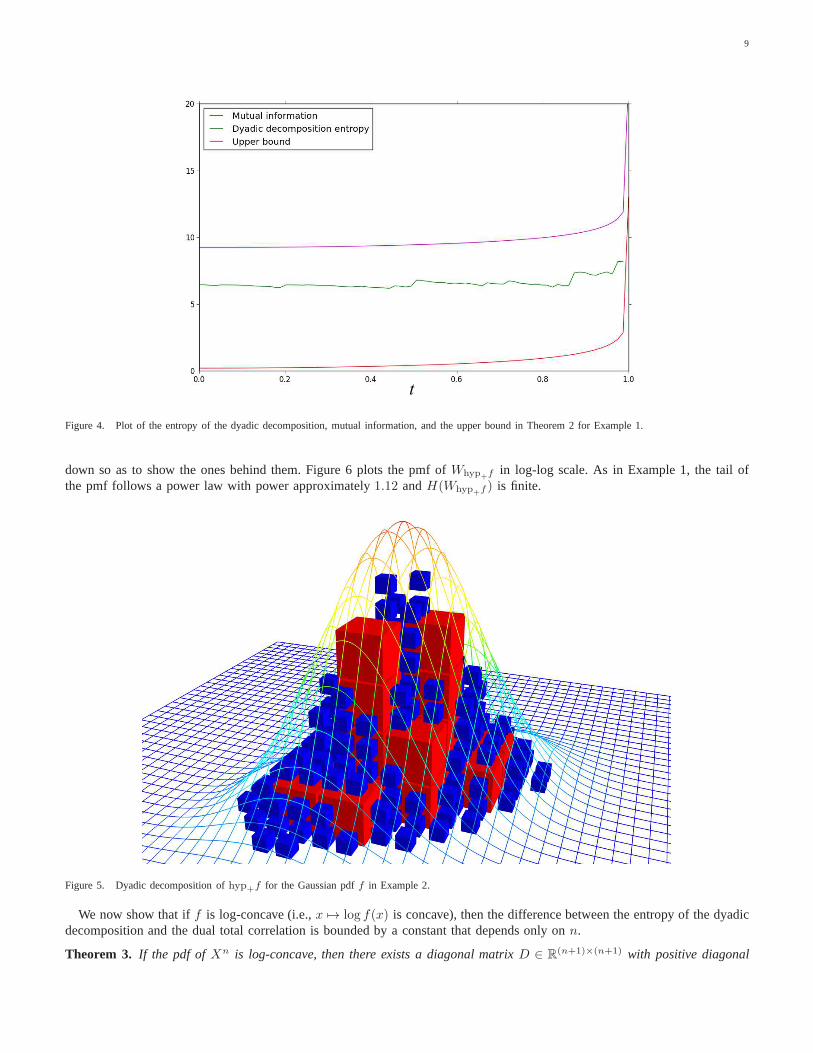
Figure 4. Plot of the entropy of the dyadic decomposition, mutual information, and the upper bound in Theorem 2 for Example 1.

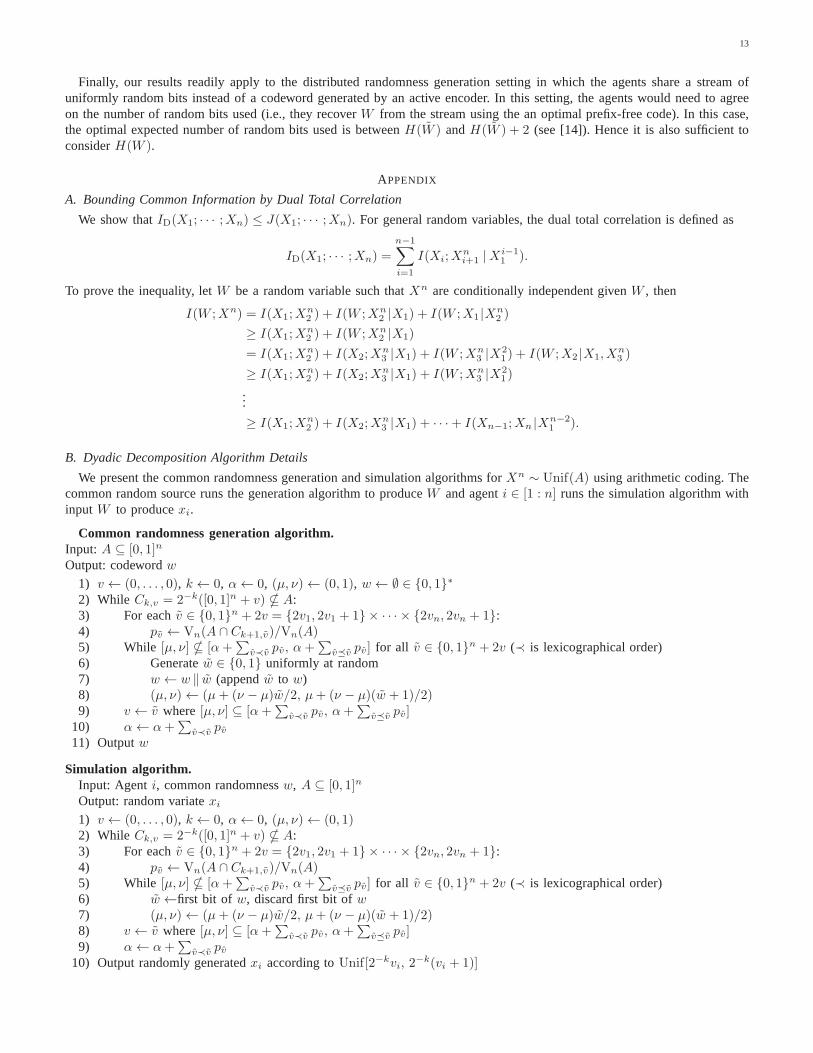
down so as to show the ones behind them. Figure 6 plots the pmf of Whyp+f in log-log scale. As in Example 1, the tail ofthe pmf follows a power law with power approximately1.12 andH(Whyp+f ) is finite.

Figure 5. Dyadic decomposition ofhyp+f for the Gaussian pdff in Example 2.

We now show that iff is log-concave (i.e.,x 7→ log f(x) is concave), then the difference between the entropy of the dyadicdecomposition and the dual total correlation is bounded by aconstant that depends only onn.

Theorem 3. If the pdf ofXn is log-concave, then there exists a diagonal matrixD ∈ R(n+1)×(n+1) with positive diagonal

10

100

101

102

103

104

105

10-7

10-6

10-5

10-4

10-3

10-2

10-1

100

Figure 6. The pmf ofW for the dyadic decomposition of the hypograph of the Gaussian pdf in Example 2.

entries such that the entropy of the dyadic decomposition ofDhyp+f satisfies

H(WDhyp+f ) ≤ ID(X1; · · · ;Xn) + n2 log e+ n (logn+ log(n+ 1) + e+ 2 log e+ 2) + 2 + log e

≤ ID(X1; · · · ;Xn) + n2 log e+ 12n logn.

Moreover, by applying the randomization in Proposition 2, we obtain

ID ≤ J ≤ G ≤ ID + n2 log e+ 9n logn.

To prove Theorem 3, we first state a result in [11], which bounds the differential entropy of a log-concave pdf by itsmaximum density.

Lemma 2. For any log-concave pdff of Xn,

− log(

supx∈Rn

f(x))

≤ h(Xn) ≤ − log(

supx∈Rn

f(x))

+ n log e.

We can generalize Lemma 2 to bound the conditional differential entropy as follows.

Lemma 3. For any log-concave pdff of Xn, and1 ≤ m ≤ n,

0 ≤ h(Xnm+1 |Xm) + log

(

ˆ

Rm

supxnm+1∈Rn−m

f(xm, xnm+1)dx

m)

≤ n log e+ log

(

n

m

)

.

The proof of this lemma is given in Appendix F.

Next, we establish a bound on the difference between the differential entropy and the truncated differential entropy.

Lemma 4. For any log-concave pdff ,

hζ(Xn)− h(Xn) ≤ log ζ + ν + n log e,

whereν ≥ 0 satisfiesΓ(n+ 1, ν) = ζ · Γ(n+ 1),

and Γ(n, z) =´∞

ztn−1e−tdt is the incomplete gamma function, andΓ(n) = Γ(n, 0) is the gamma function. Moreover, if

ζ ≥ e−(e−2)n, thenhζ(X

n)− h(Xn) ≤ log ζ + (e+ log e)n.

The proof of this lemma is given in Appendix G.

We now proceed to the proof of Theorem 3.

11

Proof of Theorem 3:Let (Xn, Z) ∼ Unif(hyp+f). Applying Theorem 2 onhyp+f , we have

H(WDhyp+f ) ≤ h1/(n+1)(Xn) +

n∑

i=1

h1/(n+1)(X[1:n]\i, Z) + (n+ 1) log(n+ 1) + (2 + log e)(n+ 1)

≤ h1/(n+1)(Xn) +

n∑

i=1

log(

VP\i(hyp+f))

+ (n+ 1) log(n+ 1) + (2 + log e)(n+ 1).

Consider the termh1/(n+1)(Xn). Since1/(n+ 1) ≥ e−(e−2)n, by Lemma (4) we have

h1/(n+1)(Xn)− h(Xn) ≤ − log(n+ 1) + (e+ log e)n.

Consider the termlog(

VP\n(hyp+f))

. By Lemma (3), we have

log(

VP\n(hyp+f))

= log

ˆ

Rn−1

supxn

f(xn−11 , xn)dx

n−11

≤ −h(Xn |Xn−11 ) + n log e+ log

(

n

n− 1

)

= −h(Xn |Xn−11 ) + n log e+ logn.

HenceH(WDhyp+f )

≤ h(Xn)− log(n+ 1) + (e+ log e)n

+n∑

i=1

(

−h(Xi |X[1:n]\i) + n log e+ logn)

+ (n+ 1) log(n+ 1) + (2 + log e)(n+ 1)

= ID(X1; · · · ;Xn) + n2 log e+ n (logn+ log(n+ 1) + e+ 2 log e+ 2) + 2 + log e.

Note that the result in Theorem 3 can be readily extended to mixtures of log-concave pdfs using the union property inProposition 1. It is not possible to obtain a constant bound on the gap betweenID andG for arbitrary pdfs, however. To

see this, let(X1, X2) ∈ {1, . . . , 2m}2 be two discrete random variables with pmf

1/3 1/3

1/3 0

⊗m

, i.e., (X1, X2) consists of

m i.i.d. copies of two random variables with pmf

1/3 1/3

1/3 0

. Now let X1 = X1 + Z1 andX2 = X2 + Z2, where

Z1, Z2 ∼ Unif[0, 1]. Then we haveI(X1;X2) = I(X1; X2) = (log 3 − 4/3)m, J(X1;X2) = J(X1; X2) = (2/3)m, and thegap betweenI andJ grows linearly inm. SinceG ≥ J , the gap betweenI andG grows at least linearly inm.

IV. A PPROXIMATE DISTRIBUTED SIMULATION

The cardinality ofW for exact simulation ofn continuous random variables is in general infinite, hence the length of thecodeword forW is unbounded. We show that if the exact simulation requirement is relaxed by only requiring that the totalvariation distance between the distributions of the simulated and the prescribed random variables to be small, then distributedsimulation is possible with a fixed length code.

We define the approximate distributed simulation problem asfollows. There aren agents that have access to commonrandomnessW ∈ {0, 1}N . Agent i ∈ [1 : n] wishes to simulate the random variableXi usingW and its local randomness,which is independent ofW and local randomness at other agents, such that the total variation between the distributions ofXn

andXn is bounded asdTV

(

(X1, . . . , Xn) , (X1, . . . , Xn))

≤ ǫ,

for someǫ > 0. The problem is to find the conditions under which the length-distance pair(N, ǫ) is achievable.We can find sufficient conditions under which(N, ǫ) is achievable by terminating the dyadic decomposition scheme described

in the previous sections after a finite number of iterations,that is, by discarding all hypercubes smaller than a prescribed size.The following proposition gives the length-distance pairsachievable by this truncated dyadic decomposition scheme in termsof H(WA) for uniform pdf overA (or H(WDhyp+f ) for non-uniform pdfs), which in turn can be bounded by Theorem 1, 2or 3.

12

Theorem 4. Let Xn ∼ Unif(A), whereA ⊆ Rn with a boundary of measure zero. The truncated dyadic decompositionscheme can achieve the length-distance pair(N, ǫ) if

N ≥ log(

ǫ2ǫ−1H(WA) + 1

)

.

Proof: Let WA be the dyadic decomposition common randomness variable forXnUnif(A) and define

WA =

{

(k, v) if k < l

(k0, v0) if k ≥ l,

whereWA = (k, v), and (k0, v0) is any hypercube with side length> 2−l, wherel = n−1(ǫ−1H(WA) − logVn(A)). Thetruncated scheme usesWA as common randomness variable, and the operations performed by the agents are unchanged. Sincethe truncated scheme differs from the original scheme only whenWA 6= WA, we have

dTV

(

(X1, . . . , Xn) , (X1, . . . , Xn))

≤ P {K ≥ l}= P {logVn(A) + nK ≥ logVn(A) + nl}

≤ E [logVn(A) + nK]

logVn(A) + nl

=H(WA)

logVn(A) + nl

= ǫ.

It is left to bound the cardinality ofWA. Consider the probability vectorpWA∈ R|WA|. SincepWA

(w) ≥ 2−nlV−1n (A),

the vectorpWAcan be expressed as a convex combination of the vectors2−nlV−1

n (A)1 +(

1− 2−nlV−1n (A)|WA|

)

ei for

i = 1, . . . , |WA|. We have

H(

2−nlV−1n (A)1+

(

1− 2−nlV−1n (A)|WA |

)

ei

)

= 2−nlV−1n (A)(|WA | − 1) · (logVn(A) + nl)−

(

1− 2−nlV−1n (A)(|WA | − 1)

)

log(

1− 2−nlV−1n (A)(|WA | − 1)

)

≥ 2−nlV−1n (A)(|WA | − 1) · (logVn(A) + nl) .

Since entropy is concave,H(WA) ≥ H(WA) ≥ 2−nlV−1n (A)(|WA| − 1) · (log Vn(A) + nl). By Theorem 3,

|WA | ≤1

logVn(A) + nl2nlVn(A)H(WA) + 1

=1

ǫ−1H(WA)2ǫ

−1H(WA)H(WA) + 1

= ǫ2ǫ−1H(WA) + 1

≤ 2N .

The result follows.

V. CONCLUSION

We proposed a scheme for distributed simulation of continuous random variables based on dyadic decomposition. Weestablished a bound on the entropy of the constructed commonrandomness in terms of the dual total correlation for the classof log concave pdfs. As a result, the gap between exact and Wyner’s common information and dual total correlation can bebounded for this set of distributions.

Our results readily translate to the exact, one-shot version of the channel synthesis problem in [5], [12] without commonrandomness in which we wish to simulate a channelfY |X(y|x) with input distributionfX(x). Given the inputX ∼ fX , theencoder produces the codewordW using a prefix-free code. Upon receivingW , the decoder produces the outputY such that(X, Y ) ∼ fXfY |X . The problem again is to find the minimum entropy ofW . A consequence of our results is that an additiveGaussian noise channel with Gaussian input, can be exactly simulated using only a finite amount of common randomness.

We have seen in Section II-A that performing different scalings on eachXi can reduceH(W ). More generally, applyinga bijective transformationgi(xi) to each random variable before using the dyadic decomposition scheme may help reduceH(W ) further. For example, applying the copula transform [13]gi(x) = FXi

(x) such thatgi(Xi) ∼ Unif[0, 1] has the benefitthat when theXi’s are close to independent, the pdf is close to a constant function over the unit hypercube, which is likelyto result in a smallerH(W ).

13

Finally, our results readily apply to the distributed randomness generation setting in which the agents share a stream ofuniformly random bits instead of a codeword generated by an active encoder. In this setting, the agents would need to agreeon the number of random bits used (i.e., they recoverW from the stream using the an optimal prefix-free code). In this case,the optimal expected number of random bits used is betweenH(W ) andH(W ) + 2 (see [14]). Hence it is also sufficient toconsiderH(W ).

APPENDIX

A. Bounding Common Information by Dual Total Correlation

We show thatID(X1; · · · ;Xn) ≤ J(X1; · · · ;Xn). For general random variables, the dual total correlation is defined as

ID(X1; · · · ;Xn) =

n−1∑

i=1

I(Xi;Xni+1 |X i−1

1 ).

To prove the inequality, letW be a random variable such thatXn are conditionally independent givenW , then

I(W ;Xn) = I(X1;Xn2 ) + I(W ;Xn

2 |X1) + I(W ;X1 |Xn2 )

≥ I(X1;Xn2 ) + I(W ;Xn

2 |X1)

= I(X1;Xn2 ) + I(X2;X

n3 |X1) + I(W ;Xn

3 |X21 ) + I(W ;X2 |X1, X

n3 )

≥ I(X1;Xn2 ) + I(X2;X

n3 |X1) + I(W ;Xn

3 |X21 )

...

≥ I(X1;Xn2 ) + I(X2;X

n3 |X1) + · · ·+ I(Xn−1;Xn |Xn−2

1 ).

B. Dyadic Decomposition Algorithm Details

We present the common randomness generation and simulationalgorithms forXn ∼ Unif(A) using arithmetic coding. Thecommon random source runs the generation algorithm to produceW and agenti ∈ [1 : n] runs the simulation algorithm withinput W to producexi.

Common randomness generation algorithm.Input: A ⊆ [0, 1]n

Output: codewordw

1) v ← (0, . . . , 0), k ← 0, α← 0, (µ, ν)← (0, 1), w← ∅ ∈ {0, 1}∗2) While Ck,v = 2−k([0, 1]n + v) * A:3) For eachv ∈ {0, 1}n + 2v = {2v1, 2v1 + 1} × · · · × {2vn, 2vn + 1}:4) pv ← Vn(A ∩ Ck+1,v)/Vn(A)5) While [µ, ν] * [α+

∑

v≺v pv, α+∑

v�v pv] for all v ∈ {0, 1}n + 2v (≺ is lexicographical order)6) Generatew ∈ {0, 1} uniformly at random7) w ← w ‖ w (appendw to w)8) (µ, ν)← (µ+ (ν − µ)w/2, µ+ (ν − µ)(w + 1)/2)9) v ← v where[µ, ν] ⊆ [α+

∑

v≺v pv, α+∑

v�v pv]10) α← α+

∑

v≺v pv11) Outputw

Simulation algorithm.Input: Agenti, common randomnessw, A ⊆ [0, 1]n

Output: random variatexi

1) v ← (0, . . . , 0), k ← 0, α← 0, (µ, ν)← (0, 1)2) While Ck,v = 2−k([0, 1]n + v) * A:3) For eachv ∈ {0, 1}n + 2v = {2v1, 2v1 + 1} × · · · × {2vn, 2vn + 1}:4) pv ← Vn(A ∩ Ck+1,v)/Vn(A)5) While [µ, ν] * [α+

∑

v≺v pv, α+∑

v�v pv] for all v ∈ {0, 1}n + 2v (≺ is lexicographical order)6) w ←first bit of w, discard first bit ofw7) (µ, ν)← (µ+ (ν − µ)w/2, µ+ (ν − µ)(w + 1)/2)8) v ← v where[µ, ν] ⊆ [α+

∑

v≺v pv, α+∑

v�v pv]9) α← α+

∑

v≺v pv10) Output randomly generatedxi according toUnif[2−kvi, 2

−k(vi + 1)]

14

The above algorithms assumeA ⊆ [0, 1]n. The case whereA is unbounded can be handled by first encoding the integer parts⌊Xn⌋ = (⌊X1⌋ , . . . , ⌊Xn⌋) of Xn ∼ Unif(A), then run the algorithms onA∩([0, 1]n+⌊Xn⌋). The algorithms can be appliedto non-uniform pdfs by lettingA to behyp+f scaled according to Theorem 2.

An advantage of the generation and simulation algorithms based on arithmetic coding is that each bit ofw is generateduniformly, and hence can be applied to the situation where the agents share a stream of uniformly random bits [14].

C. Proof of Proposition 1

The monotonicity property and the linear transformation property follow directly from the definition of erosion entropy.For the scaling property, consider

h⊖βB(αA) =

ˆ ∞

−∞

(

1 {t ≥ 0} − Vn (αA⊖ 2−tβB)

Vn(αA)

)

dt

=

ˆ ∞

−∞

(

1 {t ≥ 0} − Vn

(

A⊖ 2−t+log(β/α)B)

Vn(A)

)

dt

=

ˆ ∞

−∞

(

1 {t ≥ − log(β/α)} − Vn (A⊖ 2−tB)

Vn(A)

)

dt

≥ h⊖B(A) + log(β/α).

For the union property, consider

h⊖B

(

k⋃

i=1

Ai

)

=

ˆ ∞

−∞

(

1 {t ≥ 0} − Vn ((⋃

iAi)⊖ 2−tB)∑

i Vn(Ai)

)

dt

≤ˆ ∞

−∞

(

1 {t ≥ 0} − Vn (⋃

i (Ai ⊖ 2−tB))∑

i Vn(Ai)

)

dt

=

ˆ ∞

−∞

(

1 {t ≥ 0} −∑

iVn (Ai ⊖ 2−tB)∑

i Vn(Ai)

)

dt

=

ˆ ∞

−∞

(

∑

i

Vn(Ai)∑

j Vn(Aj)

(

1 {t ≥ 0} − Vn (Ai ⊖ 2−tB)

Vn(Ai)

)

)

dt

=∑

i

Vn(Ai)∑

j Vn(Aj)· h⊖B(Ai).

Equality holds if(⋃

iAi)⊖ 2−tB =⋃

i (Ai ⊖ 2−tB), which is true when the closures ofA1, . . . , Ak are disjoint.For the reduction to differential entropy property, letXn ∼ Unif(A), andA ∩ L is connected for any lineL parallel to the

n-th axis, then

h⊖{0}n−1×[0,1](A) =

ˆ ∞

−∞

(

1 {t ≥ 0} − Vn

(

A⊖(

{0}n−1 × [0, 2−t]))

Vn(A)

)

dt

=

ˆ ∞

−∞

(

1 {t ≥ 0} −ˆ

Rn−1

V1

((

A⊖ {0}n−1 × [0, 2−t])

∩(

{xn−11 } × R

))

Vn(A)dxn−1

1

)

dt

=

ˆ ∞

−∞

(

1 {t ≥ 0} −ˆ

Rn−1

max{

fXn−11

(xn−11 )− 2−t, 0

}

dxn−11

)

dt

=

ˆ

Rn−1

fXn−11

(xn−11 )

ˆ ∞

−∞

(

1 {t ≥ 0} −max{

1− 2−t/fXn−11

(xn−11 ), 0

})

dtdxn−11

=

ˆ

Rn−1

fXn−11

(xn−11 )

ˆ ∞

−∞

(

1 {t ≥ 0} −max{

1− 2−t/fXn−11

(xn−11 ), 0

})

dtdxn−11

=

ˆ

Rn−1

fXn−11

(xn−11 )

(

− log fXn−11

(xn−11 ) +

ˆ ∞

−∞

(

1 {t ≥ 0} −max{

1− 2−t, 0})

dtdxn−11

)

= h(Xn−11 ) + log e.

D. Proof of Proposition 2

Note thatk∑

l=−∞

2−nl |Dl(A)| = 2−nk |{v ∈ Zn : Ck,v ⊆ A}| ≥ 2−nk∣

∣

{

v ∈ Zn : Ck−1,(v−w)/2 ⊆ A}∣

∣ .

15

for any w ∈ [0, 1]n, sinceCk,v ⊆ Ck−1,(v−w)/2. Note that the(v − w)/2 in the subscript may not have integer entries, butstill the same definitionCk,v = 2−k([0, 1]n + v) can be applied. Also

ˆ

[0,1]n

∣

∣

{

v ∈ Zn : Ck−1,(v−w)/2 ⊆ A}∣

∣ dw =∑

v∈Zn

ˆ

[0,1]n1

{

Ck−1,(v−w)/2 ⊆ A}

dw

= 2nˆ

Rn

1 {Ck−1,w ⊆ A} dw

= 2n2n(k−1)Vn

(

A⊖ [0, 2−(k−1)]n)

= 2nkVn

(

A⊖ [0, 2−(k−1)]n)

.

Hencek∑

l=−∞

2−nl |Dl(A)| ≥ Vn

(

A⊖ [0, 2−(k−1)]n)

,

∞∑

l=k+1

2−nl |Dl(A)| ≤ Vn(A)−Vn

(

A⊖ [0, 2−(k−1)]n)

.

Note thatH(WA) = H(W(1/2)A), and also the right-hand-side of the proposition remains the same whenA is replaced by(1/2)A. Without loss of generality assumeA is small enough such thatVn(A) ≤ 1, soDk(A) = ∅ for k < 0.

H(WA) = logVn(A) +1

Vn(A)

∞∑

k=0

nk2−nk |Dk(A)|

= logVn(A) +n

Vn(A)

∞∑

k=0

∞∑

l=k+1

2−nl |Dl(A)|

≤ logVn(A) +n

Vn(A)

∞∑

k=0

(

Vn(A)−Vn

(

A⊖ [0, 2−(k−1)]n))

≤ logVn(A) +n

Vn(A)

ˆ ∞

−2

(

Vn(A)−Vn

(

A⊖ [0, 2−t]n))

dt

= logVn(A) + n · h⊖[0,1]n(A) + 2n.

To prove the second result, considerk∑

l=−∞

2−nl |Dl (Λ(A+ U))| = 2−nk |{v ∈ Zn : Ck,v ⊆ Λ(A+ U)}|

= 2−nk∣

∣

{

v ∈ Zn : Λ−1Ck,v − U ⊆ A}∣

∣ .

Assumingk ≥ −T and taking expectation overU , we obtain

E

[

k∑

l=−∞

2−nl |Dl (ΛA+ U)|∣

∣

∣

∣

Λ

]

= 2−nT

ˆ

[0,2T ]n2−nk |{v ∈ Zn : Ck,v − u ⊆ ΛA}| du

= 2−nT

ˆ

[0,2T ]n2−nk

∣

∣

{

v ∈ Zn : 2−k(

[0, 1]n + v − 2ku)

⊆ ΛA}∣

∣ du

=

ˆ

[0,1]n2−nk

∣

∣

{

v ∈ Zn : 2−k(

[0, 1]n + v − 2T+ku)

⊆ ΛA}∣

∣ du

(a)=

ˆ

Rn

2−nk1

{

2−k ([0, 1]n + u) ⊆ ΛA}

du

=

ˆ

Rn

1{

2−k[0, 1]n + u ⊆ ΛA}

du

= Vn

(

ΛA⊖ 2−k[0, 1]n)

= ΛnVn

(

A⊖ Λ−12−k[0, 1]n)

,

where(a) follows since2T+k is a non-negative integer. Since2nT > Vn(2A), Dk(ΛA + U) = ∅ for k < −T . Hence, wehave

H(WΛA+U ) = logVn(ΛA) +1

Vn(ΛA)

∞∑

k=−T

nk2−nk |Dk(ΛA+ U)|

16

= logVn(A) + n log Λ +n

ΛnVn(A)

∞∑

k=−T

(

1 {k ≥ 0}ΛnVn(A)−k∑

l=−∞

2−nl |Dl(ΛA+ U)|)

.

Taking expectation overU , we obtain

E[

H(WΛA+U )

∣

∣

∣

∣

Λ

]

= logVn(A) + n log Λ +n

ΛnVn(A)

∞∑

k=−T

(

1 {k ≥ 0}ΛnVn(A) − ΛnVn

(

A⊖ Λ−12−k[0, 1]n))

= logVn(A) + n log Λ + n∞∑

k=−T

(

1 {k ≥ 0} − Vn

(

A⊖ Λ−12−k[0, 1]n)

Vn(A)

)

.

Taking expectation overΛ, we have

E [H(WΛA+U )] = logVn(A) + E [n log Λ] + nE

[

∞∑

k=−T

(

1 {k ≥ 0} − Vn

(

A⊖ 2−(k+Θ)[0, 1]n)

Vn(A)

)]

= logVn(A) +n

2+ n

(

ˆ ∞

−T

(

1 {θ ≥ 0} − Vn

(

A⊖ 2−θ[0, 1]n)

Vn(A)

)

dθ − 1

2

)

= logVn(A) + n

ˆ ∞

−T

(

1 {θ ≥ 0} − Vn

(

A⊖ 2−θ[0, 1]n)

Vn(A)

)

dθ

(a)= logVn(A) + n

ˆ ∞

−∞

(

1 {θ ≥ 0} − Vn

(

A⊖ 2−θ[0, 1]n)

Vn(A)

)

dθ

= logVn(A) + n · h⊖[0,1]n(A).

where(a) follows since2nT > Vn(2A), henceA⊖ 2−θ[0, 1]n = ∅ for θ ≤ −T .

E. Proof of Theorem 2

We first prove the following claim onH(WA) involving truncated differential entropy

H(WA) ≤ n

(

H(ζ1, . . . , ζn) +

n∑

i=1

ζihζi(X[1:n]\i)

)

− (n− 1) logVn(A) + (2 + log e)n,

whereζi =

ˆ

Rn−1

min{

fX[1:n]\i(x[1:n]\i) , ξ

}

dx[1:n]\i

for a suitableξ > 0 such that∑

ζi = 1. By Proposition 2, the claim can be proved by boundingh⊖[0,1]n(A). Note that byLemma 1,

h⊖[0,1]n(A) =

ˆ ∞

−∞

(

1 {t ≥ 0} − Vn (A⊖ [0, 2−t]n)

Vn(A)

)

dt

≤ˆ ∞

−∞

(

1 {t ≥ 0} − 1

Vn(A)max

(

0, Vn(A)−n∑

i=1

ˆ

P\i(A)

min{

2−t , V1 (A ∩ (span(ei) + x))}

dx[1:n]\i

))

dt

=

ˆ ∞

−∞

(

1 {t ≥ 0} −max

(

0, 1−n∑

i=1

ˆ

P\i(A)

min

{

2−t

Vn(A), fX[1:n]\i

(x[1:n]\i)

}

dx[1:n]\i

))

dt

(a)=

ˆ ∞

−∞

(

−1 {t < 0}+n∑

i=1

ˆ

P\i(A)

min

{

2−t

Vn(A), ξ, fX[1:n]\i

(x[1:n]\i)

}

dx[1:n]\i

)

dt

=n∑

i=1

ˆ ∞

−∞

(

−1 {t < 0} · ζi +ˆ

P\i(A)

min

{

2−t

Vn(A), ξ, fX[1:n]\i

(x[1:n]\i)

}

dx[1:n]\i

)

dt

=

n∑

i=1

ˆ

P\i(A)

ˆ ∞

−∞

(

−1 {t < 0} ·min{

ξ, fX[1:n]\i(x[1:n]\i)

}

+min

{

2−t

Vn(A), ξ, fX[1:n]\i

(x[1:n]\i)

})

dtdx[1:n]\i

=

n∑

i=1

ˆ

P\i(A)

−min{

ξ, fX[1:n]\i(x[1:n]\i)

}

·(

log(

Vn(A)min{

ξ, fX[1:n]\i(x[1:n]\i)

})

− log e)

dx[1:n]\i

= − logVn(A) +H(ζ1, . . . , ζn)

17

+

n∑

i=1

ζi

ˆ

P\i(A)

−ζ−1i min

{

ξ, fX[1:n]\i(x[1:n]\i)

}

· log(

ζ−1i min

{

ξ, fX[1:n]\i(x[1:n]\i)

})

dx[1:n]\i + log e

= − logVn(A) +H(ζ1, . . . , ζn) +

n∑

i=1

ζihζi(X[1:n]\i) + log e,

where(a) follows by the definition ofξ. The claim follows.We proceed to prove Theorem 2. LetD = diag(d1, . . . , dn). Assuming

∏

i di = 1, then by the claim,

H(WDA) ≤ n

H(ζ1, . . . , ζn) +

n∑

i=1

ζi

hζi(X[1:n]\i) +∑

j 6=i

log dj

− (n− 1) logVn(A) + (2 + log e)n

≤ n

n∑

i=1

ζi

(

hζi(X[1:n]\i)− log di

)

− (n− 1) logVn(A) + n logn+ (2 + log e)n,

where

ζi =

∏

j 6=i

dj

ˆ

Rn−1

min

∏

j 6=i

dj

−1

fX[1:n]\i(x[1:n]\i) , ξ

dx[1:n]\i

=

ˆ

Rn−1

min{

fX[1:n]\i(x[1:n]\i) , ξd

−1i

}

dx[1:n]\i

for a suitableξ > 0 such that∑

ζi = 1. Let α1, . . . , αn > 0 such thatˆ

Rn−1

min{

fX[1:n]\i(x[1:n]\i) , αi

}

dx[1:n]\i =1

n.

Setξ =(

∏

j aj

)1/n

, di = α−1i ξ, then we haveζi = 1/n,

H(WDA) ≤n∑

i=1

h1/n(X[1:n]\i)− (n− 1) logVn(A) + n logn+ (2 + log e)n.

F. Proof of Lemma 3

Before proving this lemma, we first prove the following claimon the volume of a convex set. For any convex setA ⊆ Rn

where0 ∈ A and1 ≤ m ≤ n, let A ={

xnm+1 : (0m, xn

m+1) ∈ A}

, then

Vn(A) ≥(

n

m

)−1

·Vn−m(A) ·VP[1:m](A).

Now we prove the claim. Denote the section ofA as

SA(xnm+1) =

{

xm : (xm, xnm+1) ∈ A

}

⊆ Rm.

Note that

Vn(A) =

ˆ

Sm−1

ˆ ∞

0

(

ˆ

{xnm+1: (rx

m, xnm+1)∈A}

dxnm+1

)

rm−1drdxm

=

ˆ

Sm−1

ˆ

{(r, xnm+1): r≥0, (rxm, xn

m+1)∈A}rm−1d(r, xn

m+1)dxm.

Consider the setSrad,A(x

m) ={

(r, xnm+1) : r ≥ 0, (rxm, xn

m+1) ∈ A}

.

It is the intersection ofA and a half-space, and hence it is convex. By definition of radial function and projection, there existsxnm+1(x

n) such that(ρP[1:m](A)(x

m), xnm+1(x

n)) ∈ Srad,A(xm).

Also by definition ofA,{0} × A ⊆ Srad,A(x

m).

18

Hence the convex hull of{

(ρP[1:m](A)(xm), xn

m+1(xn))}

∪(

{0} × A)

is a subset ofSrad,A(xm). The convex hull can be

expressed as{

(r, xnm+1) : 0 ≤ r ≤ ρP[1:m](A)(x

m), xnm+1 ∈

(

1− rρ−1P[1:m](A)(x

m))

A+ rρ−1P[1:m](A)(x

m) · xnm+1(x

n)}

.

Therefore,

Vn(A) =

ˆ

Sm−1

ˆ

Srad,A(xm)

rm−1d(r, xnm+1)dx

m

≥ˆ

Sm−1

ˆ ρP[1:m](A)(xm)

0

ˆ

(

1−rρ−1P[1:m](A)

(xm)

)

A+rρ−1P[1:m](A)

(xm)·xnm+1(x

n)

dxnm+1 · rm−1drdxm

=

ˆ

Sm−1

ˆ ρP[1:m](A)(xm)

0

Vn−m(A)(

1− rρ−1P[1:m](A)(x

m))n−m

rm−1drdxm

=

ˆ

Sm−1

ρmP[1:m](A)(xm)Vn−m(A) · B(m, n−m+ 1)dxm

= m · B(m, n−m+ 1) · Vn−m(A) · VP[1:m](A),

where

B(α, β) =

ˆ 1

0

tα−1(1− t)β−1dt

is the beta function. The claim follows.We proceed to prove Lemma 3. To prove the lower bound, consider

h(Xnm+1 |Xm) =

ˆ

Rm

fXm(xm)h(Xnm+1 |Xm = xm)dxm

≥ˆ

Rm

fXm(xm) · − log supxnm+1∈Rn−m

f(xnm+1 | xm)dxm

≥ − log

ˆ

Rm

fXm(xm) supxnm+1∈Rn−m

f(xnm+1 | xm)dxm

= − log

ˆ

Rm

supxnm+1∈Rn−m

f(xm, xnm+1)dx

m.

Now we prove the upper bound. By Lemma 2,

h(Xn) ≤ − log(

supxn∈Rn

f(xn))

+ n log e, (7)

h(Xm) ≥ − log(

supxm∈Rm

fXm(xm))

. (8)

Without loss of generality, assume thatsupxm∈Rm fXm(xm) is attained atxm = 0 and supxnm+1

f(0m, xnm+1) is attained at

xnm+1 = 0. Denote the super level set

L+z (f) = {xn : f(xn) ≥ z} .

Sincef is log-concave,L+z (f) is convex. Define

L+z (f) =

{

xnm+1 : (0m, xn

m+1) ∈ L+z (f)

}

.

By the claim we proved earlier,ˆ

Rn

f(xn) =

ˆ ∞

0

Vn

(

L+z (f)

)

dz

≥ˆ

{z: 0∈L+z (f)}

Vn

(

L+z (f)

)

dz

≥ˆ

{z: 0∈L+z (f)}

(

n

m

)−1

· Vn−m(L+z (f)) ·VP[1:m](L

+z (f))dz

=

(

n

m

)−1

·ˆ f(0)

0

Vn−m(L+z (f)) ·VP[1:m](L

+z (f))dz

19

(a)

≥(

n

m

)−1

·(

ˆ f(0)

0

Vn−m(L+z (f))dz

)

·(

1

f(0)

ˆ f(0)

0

VP[1:m](L+z (f))dz

)

(b)

≥(

n

m

)−1

· fXm(0) ·(

1

supx f(x)

ˆ supx f(x)

0

VP[1:m](L+z (f))dz

)

=

(

n

m

)−1

· fXm(0) · 1

supx f(x)

ˆ

Rm

supxnm+1∈Rn−m

f(xm, xnm+1)dx

m

(c)

≥(

n

m

)−1

· 2−h(Xm) · 2h(Xn)e−n

ˆ

Rm

supxnm+1∈Rn−m

f(xm, xnm+1)dx

m.

where (a) is due to Chebyshev’s sum inequality, since bothVn−m(L+z (f)) andVP[1:m](L

+z (f)) are non-increasing inz,

(b) is due to´ f(0)

0Vn−m(L+

z (f))dz =´

Rn−m f(0m, xnm+1)dx

nm+1 = fXm(0) since supxn

m+1f(0m, xn

m+1) = f(0), andVP[1:m](L

+z (f)) dz is non-increasing inz, and(c) is due to (7) and (8). The result follows from

´

Rn f(xn) = 1.

G. Proof of Lemma 4

As in the definition ofhζ , let ξ > 0 such thatˆ

Rn

min {ξ, f(x)} dx = ζ.

Without loss of generality, assumesupx∈Rn f(x) = f(0) and letα = f(0). Let

A = {x ∈ Rn : f(x) ≥ ξ} .By log-concavity off , we knowA is convex, and we have

Vn(A) =1

n·ˆ

Sn−1

ρnA(x)dx,

whereSn−1 = {x ∈ Rn : ‖x‖2 = 1} is the unit sphere. Forx ∈ A, by definition ofρA, we knowx/(ρ−1A (x) + ǫ) ∈ A for

any ǫ > 0,

f(x) = f

(

(

1− ρ−1A (x)− ǫ

)

· 0 +(

ρ−1A (x) + ǫ

)

· x

ρ−1A (x) + ǫ

)

≥ (f(0))1−ρ−1

A(x)−ǫ ·

(

f

(

x

ρ−1A (x) + ǫ

))ρ−1A

(x)+ǫ

≥ α1−ρ−1A

(x)−ǫξρ−1A

(x)+ǫ.

Thereforef(x) ≥ α1−ρ−1

A(x)ξρ

−1A

(x).

Henceˆ

A

f(x)dx =

ˆ

Sn−1

ˆ ρA(x)

0

f(rx) · rn−1drdx

≥ˆ

Sn−1

ˆ ρA(x)

0

α1−ρ−1A

(rx)ξρ−1A

(rx)rn−1drdx

=

ˆ

Sn−1

ˆ ρA(x)

0

α1−rρ−1A

(x)ξrρ−1A

(x)rn−1drdx

=

ˆ

Sn−1

ρnA(x)

ˆ 1

0

α1−rξrrn−1drdx

=

ˆ

Sn−1

ρnA(x)(

α (− log(ξ/α))−n

(Γ(n)− Γ(n, − log(ξ/α))))

dx

= nα (− log(ξ/α))−n (Γ(n)− Γ(n, − log(ξ/α))) Vn(A),

whereΓ(n, z) =´∞

z tn−1e−tdt is the incomplete gamma function, andΓ(n) = Γ(n, 0) is the gamma function.On the other hand, forx /∈ A, then for anyǫ > 0, we havex/(ρ−1

A (x) − ǫ) /∈ A,

ξ ≥ f

(

x

ρ−1A (x) − ǫ

)

= f

((

1− 1

ρ−1A (x)− ǫ

)

· 0 + 1

ρ−1A (x) − ǫ

· x)

≥ α1−1/(ρ−1A

(x)−ǫ) · (f(x))1/(ρ−1A

(x)−ǫ) ,

20

Thereforef(x) ≤ α1−ρ−1

A(x)ξρ

−1A

(x).

Henceˆ

Rn\A

f(x)dx =

ˆ

Sn−1

ˆ ∞

ρA(x)

f(rx) · rn−1drdx

≤ˆ

Sn−1

ˆ ∞

ρA(x)

α1−ρ−1A

(rx)ξρ−1A

(rx)rn−1drdx

=

ˆ

Sn−1

ˆ ∞

ρA(x)

α1−rρ−1A

(x)ξrρ−1A

(x)rn−1drdx

=

ˆ

Sn−1

ρnA(x)

ˆ ∞

1

α1−rξrrn−1drdx

=

ˆ

Sn−1

ρnA(x)(

α (− log(ξ/α))−n Γ(n, − log(ξ/α)))

dx

= nα (− log(ξ/α))−n

Γ(n, − log(ξ/α))Vn(A).

Recall that´

Rn min {ξ, f(x)} dx = ζ,

ζ =

ˆ

Rn

min {ξ, f(x)} dx

=

ˆ

Rn\A

f(x)dx + ξVn(A)

≤(

nα (− log(ξ/α))−n

Γ(n, − log(ξ/α)) + ξ)

Vn(A).

Alsoζ =

ˆ

Rn

min {ξ, f(x)} dx

= 1−ˆ

A

f(x)dx+ ξVn(A)

≤ 1−(

nα (− log(ξ/α))−n

(Γ(n)− Γ(n, − log(ξ/α)))− ξ)

Vn(A).

Let ν = − log(ξ/α). Sinceζ ≤ ac andζ ≤ 1− bc implies ζ ≤ a/(a+ b), we have

ζ ≤ nαν−nΓ(n, ν) + ξ

(nαν−nΓ(n, ν) + ξ) + (nαν−n (Γ(n)− Γ(n, ν))− ξ)

=nΓ(n, ν) + e−ννn

nΓ(n)

=Γ(n+ 1, ν)

Γ(n+ 1).

By Lemma 2,h(Xn) ≥ − logα. Recall thathζ(Xn) is the entropy of the pdff(x) = ζ−1 min {ξ, f(x)}, which is also

log-concave. Hence by Lemma 2,hζ(Xn) ≤ − log(ζ−1ξ) + n log e. As a result,

hζ(Xn)− h(Xn) ≤ − log

(

ζ−1ξ/α)

+ n log e

≤ log ζ + ν + n log e.

To prove the second bound, assume thatζ ≥ e−(e−2)n andν > en. We use the bound

Γ(a, z) < Bza−1e−z

for a > 1, B > 1, z > B(a− 1)/(B − 1) due to [15].Substitutinga = n + 1, z = en, andB = e, we haveΓ(n + 1, ν) < Γ(n + 1, en) < e(en)ne−en. We also know that

Γ(n+ 1) ≥ nne−(n−1), henceΓ(n+ 1, ν)

Γ(n+ 1)<

e(en)ne−en

nne−(n−1)

= e−(e−2)n,

which leads to a contradiction andν ≤ en. The result follows.

21

REFERENCES

[1] G. R. Kumar, C. T. Li, and A. El Gamal, “Exact common information,” in Proc. IEEE Symp. Info. Theory. IEEE, 2014, pp. 161–165.[2] T. Linder, V. Tarokh, and K. Zeger, “Existence of optimalprefix codes for infinite source alphabets,”IEEE Trans. Info. Theory, vol. 43, no. 6, pp.

2026–2028, 1997.[3] P. Harsha, R. Jain, D. McAllester, and J. Radhakrishnan,“The communication complexity of correlation,” inProc. 22nd Ann. IEEE Conf. Computational

Complexity. IEEE, 2007, pp. 10–23.[4] A. D. Wyner, “The common information of two dependent random variables,”IEEE Trans. Inf. Theory, vol. 21, no. 2, pp. 163–179, Mar. 1975.[5] P. Cuff, H. Permuter, and T. M. Cover, “Coordination capacity,” IEEE Trans. Info. Theory, vol. 56, no. 9, pp. 4181–4206, 2010.[6] W. Liu, G. Xu, and B. Chen, “The common information ofN dependent random variables,” inProc. 48th Ann. Allerton Conf. Commun., Contr., and

Comput. IEEE, 2010, pp. 836–843.[7] G. Xu, W. Liu, and B. Chen, “Wyner’s common information for continuous random variables–a lossy source coding interpretation,” in Proc. 45th Ann.

Conf. Information Sciences and Systems. IEEE, 2011, pp. 1–6.[8] S. Satpathy and P. Cuff, “Gaussian secure source coding and Wyner’s common information,”arXiv preprint arXiv:1506.00193, 2015.[9] P. Yang and B. Chen, “Wyner’s common information in Gaussian channels,” inProc. IEEE Symp. Info. Theory. IEEE, 2014, pp. 3112–3116.

[10] T. S. Han, “Nonnegative entropy measures of multivariate symmetric correlations,”Information and Control, vol. 36, pp. 133–156, 1978.[11] S. Bobkov and M. Madiman, “The entropy per coordinate ofa random vector is highly constrained under convexity conditions,” IEEE Trans. Info.

Theory, vol. 57, no. 8, pp. 4940–4954, 2011.[12] P. Cuff, “Distributed channel synthesis,”IEEE Trans. Info. Theory, vol. 59, no. 11, pp. 7071–7096, 2013.[13] M. Sklar, Fonctions de répartition à n dimensions et leurs marges. Université Paris 8, 1959.[14] D. E. Knuth and A. C. Yao, “The complexity of nonuniform random number generation,”Algorithms and complexity: new directions and recent results,

pp. 357–428, 1976.[15] P. Natalini and B. Palumbo, “Inequalities for the incomplete gamma function,”Math. Inequal. Appl, vol. 3, no. 1, pp. 69–77, 2000.