1

Data MiningChapter 3

Output: Knowledge Representation

Kirk Scott

2

3

4

5

6

7

8

Introduction

9

• Deciding what kind of output you want is the first step towards picking a mining algorithm

• The section headings for this set of overheads are given on the following overhead

• They summarize the choices of output type available from standard data mining algorithms

10

• 3.1 Tables• 3.2 Linear Models (regression equations)• 3.3 Trees (decision trees)• 3.4 Rules (rule sets)• 3.5 Instance-Based Representation• 3.6 Clusters

11

3.1 Tables

12

• Output can be in the form of tables• This is quite straightforward and simple• Instances can be organized to form a

lookup table for classification• The contact lens data can be viewed in

this way

13

• In effect, the idea is that organized instances are a representation of the structure of the data

• At the end of the chapter the book will consider another way in which the instance set itself is pretty much the result of mining

14

3.2 Linear Models

15

• For problems with numeric attributes you can apply statistical methods

• The computer performance example was given earlier

• The methods will be given in more detail in chapter 4

• The statistical approach can be illustrated graphically

16

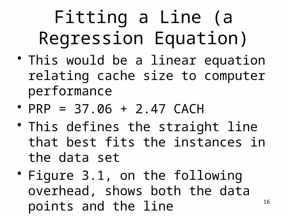
Fitting a Line (a Regression Equation)

• This would be a linear equation relating cache size to computer performance

• PRP = 37.06 + 2.47 CACH• This defines the straight line that best fits

the instances in the data set• Figure 3.1, on the following overhead,

shows both the data points and the line

17

18

Finding a Boundary

• A different technique will find a linear decision boundary

• This linear equation in petal length and petal width will separate instances of Iris setosa and Iris versicolor

• 2.0 – 0.5 PETAL_LENGTH – 0.8 PETAL_WIDTH = 0

19

• An instance of Iris setosa should give a value >0 (above/to the right of the line) and an instance of Iris versicolor should give a value <0

• Figure 3.2, on the following overhead, shows the boundary line and the instances of the two kinds of Iris

20

21

• It should be noted that the iris data set gives an amazingly clean separation of clusters or classifications in this way

• In that sense, it is both ideal and kind of artificial

• In practice, separations are not always so clear-cut

22

3.3 Trees

23

• Recall the different kinds of data:• 1. Nominal• 2. Ordinal• 3. Interval• 4. Ratio• In trees, essentially, a decision is made at

each node based on the value of a single attribute

24

• The book summarizes the different kinds of decisions (< , =, etc.) that might be coded the different kinds of data

• Most of the possible comparisons are apparent for the different kinds of data types and will not be repeated here

• Several more noteworthy aspects will be addressed on the following overheads

25

Null Values

• A given instance in a data set may have a null value for one of its attributes

• The basic logic of a decision tree is that at some node in the tree it will be necessary to branch depending on the value of that attribute

• You can’t ignore the null value when developing a decision tree or applying it

26

• The occurrence of a null value may be treated as one individual branch of several out of a decision tree node

• At this point it becomes apparent that it is useful if null can be assigned a more specific meaning like not available, not applicable, not important…

• If this is possible, it is desirable

27

• If it’s not possible to assign a meaning to nulls, then it’s necessary to have a an approach to dealing with them when analyzing the data and making the tree

• One simple approach:• Keep track of the number of instances that

fall in each branch coming out of a node, and classify nulls with the most popular branch

28

• Another, potentially better approach:• Keep track of the relative frequency of

different branches• In the aggregate results, assign a

corresponding proportion of the nulls to the different branches

29

• Neither of these approaches specifies what to do with a data item that contains nulls when applying the decision tree

• But they both are designed to make sure that when analyzing the data, each data item is taken into account, and the goal is to assign the proper “weight” to each branch based on the count of items that fall in that branch

30

Other Kinds of Comparisons

• Simple decisions compare attribute values and constants

• Some decisions may compare two attributes in the same instance

• Some decisions may be based on a function of >1 attribute per instance

31

Oblique Splits

• Comparing an attribute to a constant splits data parallel to an axis

• A decision function which doesn’t split parallel to an axis is called an oblique split

• The boundary between the kinds of irises shown earlier is such a split

• Visually, it was oblique, not parallel• The split was along a line, but the line had

its own location and slope in the plane

32

Option Nodes

• A single node with alternative splits on different attributes is called an option node

• This is not terribly difficult, but it is a step further in the direction of complexity

• To me it seems like a clear-cut case of making up rules of thumb to handle special cases because the straightforward approach doesn’t seem to be working well in practice

33

• The idea is this:• You reach a level in the tree and you have

a node where you could classify according the value of one attribute or another

• Rather than deterministically deciding to do the classification on one or the other, you do it on both attributes

34

• This is the obvious end result:• Instances end up being put in more than

one branch• Or if you’re at the bottom of the tree,

instances may appear in >1 leaf classification

• The last part of analysis includes deciding what such results indicate

35

• In other words, you’re using a half-baked rule of thumb when making a decision at a node

• Now you need a rule of thumb to decide where the multiply-classified instance actually belongs

• The solution (as is often the case) may be based on counting the relative frequency of instances in the different classifications

36

Weka and Hand-Made Decision Trees

• The book suggests that you can get a handle on decision trees by making one yourself

• The book illustrates how Weka includes tools for doing this

• To me this seems out of place until chapter 11 when Weka is introduced

• I will not cover it here

37

Regression Trees

• The general discussion of trees centers on classification—categorization at each node based on attribute values

• For a problem with numeric attributes it’s possible to devise a tree-like classifier that gives numeric results

• This is called a regression tree (which is kind of a misnomer, since no regression may be involved)

38

• The upper nodes in the tree still work like before—essentially classification

• Because the attributes of the instances are numeric, the internal nodes contain numeric comparisons of attribute values

• As a result of working through the tree, certain instances end up in each leaf

39

• The instances in each leaf may not have exactly the same value for the numeric dependent variable

• The prediction value assigned to any instance placed there will be the average of all instances placed there

40

• Stated in terms of the performance example, the leaves contain the performance prediction

• The prediction is the average of the performance of all instances that end up classified in that leaf

41

Model Trees

• A model tree is a hybrid of a decision tree and regression (as opposed to the regression tree, which doesn’t involve regression…)

• In a model tree, instances are classified into a given leaf

• Then the prediction is made by applying a linear equation to some subset of instance attribute values

42

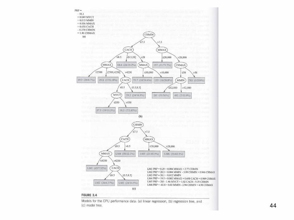
• Figure 3.4, shown on the overhead following the next one, shows (a) a linear model, (b) a regression tree, and (c) a model tree

• In the trees the leaves show the predicted value (and the number of instances/percent of instances in the leaf)

• The linear model is simple

43

• The regression tree is complex, but when you calculate the error, it is much better than the linear model

• This tells you that the data is not really linear

• The model tree is effectively a piece-wise linear model

• Different equations are right in different regions of the data space

44

45

Rule Sets from Trees

• Given a decision tree, you can generate a corresponding set of rules

• Start at the root and trace the path to each leaf, recording the conditions at each node

• The rules in such a set are independent• Each covers a separate case

46

• The rules don’t have to be applied in a particular order

• The downside is such a rule set is more complex than an ordered set

• It is possible to prune a set derived from a tree to remove redundancy

47

Trees from Rule Sets

• Given a rule set, you can generate a decision tree

• Now we’re interested in going in the opposite direction

• Even a relatively simple rule set can lead to a messy tree

48

• A rule set may compactly represent a limited number of explicitly known cases

• The other cases may be implicit in the rule set

• The implicit cases have to be spelled out in the tree

49

An Example

• Take this situation for example:• There are 4 independent binary (yes/no)

variables, a, b, c, d• There is a fourth, independent binary

classification variable, x (classify x or not x)

50

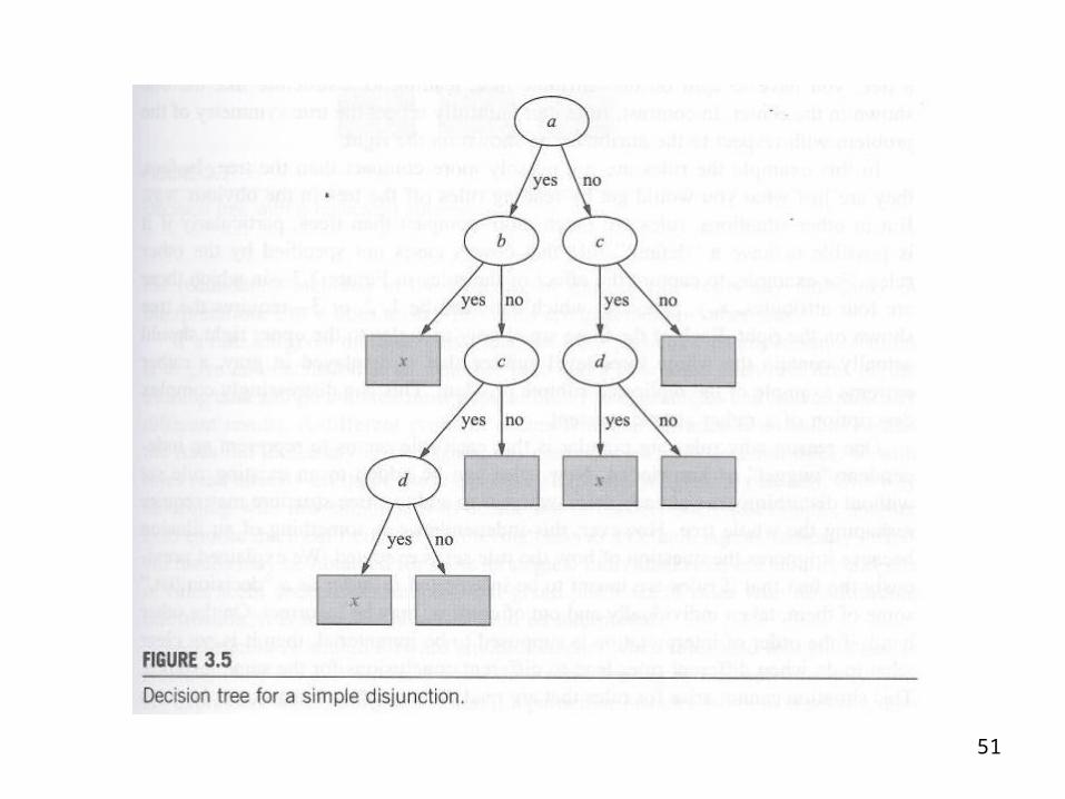
• Take this as the rule set for example:• If a and b then x• If c and d then x• With 4 variables, a, b, c, and d, there can

be up to 4 levels in the tree• A tree for this problem is shown in Figure

3.5 on the following overhead

51

52

Messiness = Replicated Subtrees

• The point is that the tree is messy compared to the rule set

• In two compact statements, the rule set tells what we know (in a positive sense)

• The outcome of all other cases (the negative cases) is implicit

53

• The tree is messy because it contains replicated subtrees

• Starting at the top, you make a decision based on a

• If a = no, you then have to test c and d • If a = yes and b = no, you have to do

exactly the same test on c and d

54

• There are two c nodes• The sub-trees on the lower left and on the

right branch from them• These sub-trees are completely analogous• They are replicated sub-trees

55

• The book states that “decision trees cannot easily express the disjunction implied among the different rules in a set.”

• Translation:• The rule set could be more completely

stated in this way:• If a and b OR if c and d

56

• The first part of the rule deals only with a and b

• The other rule is disjoint from the first rule; it deals only with b and c

• If a is no, you have to test c and d• Also, if b is no, you have to test c and d• This leads to replicated branches in the

tree representation

57

Another Example of Replicated Sub-trees

• Figure 3.6, on the following overhead, illustrates an exclusive or (XOR) function

58

59

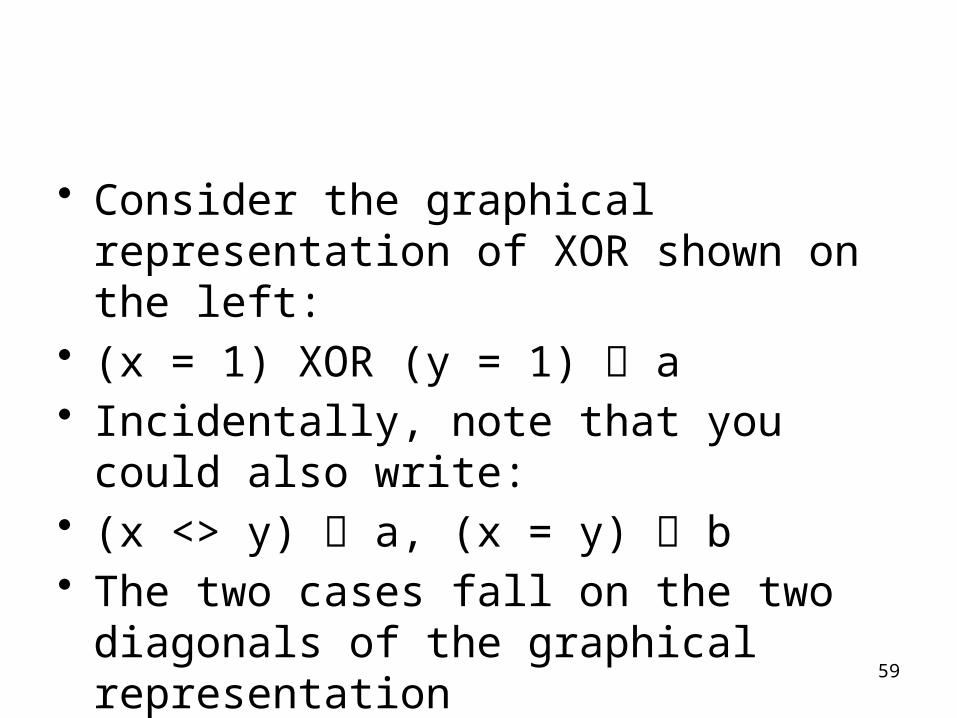
• Consider the graphical representation of XOR shown on the left:

• (x = 1) XOR (y = 1) a• Incidentally, note that you could also write:• (x <> y) a, (x = y) b• The two cases fall on the two diagonals of

the graphical representation• XOR is the case where x <> y

60

• Now consider the tree:• There’s nothing surprising: First test x,

then test y• The gray leaves on the left and the right at

the bottom are analogous• Now consider the rule set:• In this example the rule set is not simpler• This doesn’t negate the fact that the tree

has replication

61

Yet Another Example of a Replicated Sub-tree

• Consider Figure 3.7, shown on the following overhead

62

63

• In this example there are again 4 attributes• This time they are 3-valued instead of

binary• There are 2 disjoint rules, each including 2

of the variables• There is a default rule for all other cases

64

• The replication is represented in the diagram in this way:

• Each gray triangle stands for an instance of the complete sub-tree on the lower left which is shown in gray

65

• The rule set would be equally complex IF there were a rule for each branch of the tree

• It is less complex in this example because of the default rule

66

Other Issues with Rule Sets

• If you generate rules from trees, the rules will be mutually exclusive and consistent

• We have not seen the data mining algorithms yet, but some do not generate rule sets in a way analogous to reading all of the cases off of a decision tree

• Rule sets may be generated that contain conflicting rules that classify specific cases into different categories

67

• Conflicting rules can exist in sets that have to be applied in a specified order—where the order of application makes the conflict apparent rather than real

• Conflicting rules can also exist in sets where the order is not specified

• In this case, you have to have a rule of thumb for dealing with this

68

Rule Sets that Produce Multiple Classifications

• In practice you can take two approaches:• Simply do not classify instances that fall

into >1 category• Or, count how many times each rule is

triggered by a training set and use the most popular of the classification rules when two conflict

• (In effect, you’re throwing one of the rules out)

69

Rule Sets that Don’t Classify Certain Cases

• If a rule set doesn’t classify certain cases, there are again two alternatives:

• Do not classify those instances• Classify those instances with the most

frequently occurring instances

70

The Simplest Case with Rule Sets

• Suppose all variables are Boolean• I.e., suppose rules only have two possible

outcomes, T/F• Suppose only rules with T outcomes are

expressed• (By definition, all unexpressed cases are

F)

71

• Under the foregoing assumptions:• The rules are independent• The order of applying the rules is

immaterial• The outcome is deterministic• There is no ambiguity

72

Reality is More Complex

• In practice, there can be ambiguity• The authors state that the assumption that

there are only two cases, T/F, and only T is expressed, is a form of closed world assumption

• In other words, the assumption is that everything is binary

73

• As soon as this and any other simplifying assumptions are relaxed, things become messier

• In other words, rules become dependent, the order of application matters, etc.

• This is when you can arrive at multiple classifications or no classifications from a rule set

74

Association Rules

• This subsection is largely repetition• Any subset of attributes may predict any

other subset of attributes• Association rules are really just a

generalization or superset of classification rules

75

• This is the explanation:• This is the form of a classification rule:• (all non-class attributes) (class attribute)• This is just one of many rules of this form:• (one or more non-class attributes) (class

attribute or one or more attributes in general)

76

Support and Confidence (Again)

• Support = proportion of instances where the protasis occurs

• Confidence = proportion of instances where the apodosis occurs with the protasis

77

Terminology (Again)

• In general, the book uses the term Coverage = Support

• The book seems to define coverage somewhat differently in this section

• Ignore what the book says and let coverage = support

• In general, the book uses the term Accuracy = Confidence

78

Interesting Rules

• Because so many association rules are possible, you need criteria for defining interesting ones

• Association Rules are considered interesting if:

• They exceed some threshold for support• They exceed some threshold for

confidence

79

Relative Strength of Association Rules

• An association rule that implies another association rule is stronger than the rule it implies

• The stronger rule should be reported• It is not necessary to report the weaker

rule(s)• The book illustrates this idea with a

concrete weather example• It will be presented below in general form

80

An Example of an Association Rule Implying Another

• Let Rule 1 be given as shown below

• Rule 1: If A = 1 and B = 0• Then X = 0 and Y = 1

• Suppose that Rule 1 meets thresholds for support and confidence so that it’s considered interesting

81

• Now consider Rule 2:

• Rule 2: If A = 1 and B = 0• Then X = 0

• The protasis is the same as for Rule 1• It applies to the same cases as Rule 1• Therefore it has the same level of support

82

• Rule 1 has a compound conclusion:• Then X = 0 and Y = 1• Rule 2 has a single conclusion:• Then X = 0• Rule 2’s conclusion is less restrictive than

Rule 1’s conclusion• It can be true in no fewer cases than Rule

1’s conclusion

83

• This means the confidence for Rule 2 can be no less than the confidence for Rule 1

• This means that Rule 2 meets the confidence criterion for an interesting rule

• However, by the same token, it is clear that Rule 1 subsumes Rule 2

84

• Or you could say that Rule 1 implies Rule 2

• [ (Rule 1) (Rule 2) ]• But Rule 2 doesn’t imply Rule 1• (If they both implied each other, they

would be the same rule)

85

• The end result of this:• Rule 1 is the stronger rule• Therefore, when reporting association

rules, Rule 1 should be reported but Rule 2 and Rule 3 should not be reported

86

• Note that this example could also give another, analogous illustration

• Rule 1 could also be said to imply a Rule 3:

• Rule 3: If A = 1 and B = 0• Then Y = 1• Rule 1 is also stronger than Rule 3, so you

still only need to report Rule 1

87

• The conclusion to this is really kind of simple

• Association rule mining may generate many different rules

• If there are multiple rules with the same protasis, just make one rule, gathering together all of the respective apodoses and combining them with conjunction

88

Rules with Exceptions

• A data set may be mined for rules• New instances may arrive which the rule

set doesn’t correctly classify• The new instances can be handled by

adding “exceptions” to the rules

89

• Adding exceptions has this advantage:• It is not necessary to re-do the mining and

make wholesale changes to the existing rule set

• Logically, it’s not so clear what it means to mine rules but then say that they have exceptions

• How many exceptions are needed before the rule itself is negated?...

90

The Iris Exception Example

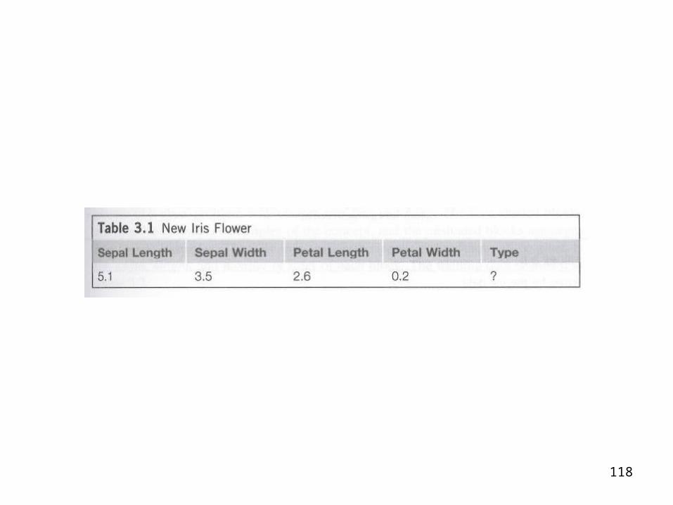
• The book illustrates exceptions with a new instance for the iris data set

• In Figure 3.8, the amended rules are expressed in terms of default cases, exceptions, and if/else rules

• Comments will follow

91

92

• It seems to me that this presentation of information as default followed by exception could be expressed in another way

• To me it would make more sense to say:• If ‘exception’ then y• Else default• If find the expressions as given using

defaults hard to understand

93

• The book observes that exceptions may be “psychologically”, if not logically preferable

• The use of exceptions may better mirror how human beings model the situation

• It may even reflect the thinking of an informed expert more closely than a re-done set of rules

94

More Expressive Rules

• Simple rules compare attributes with constants

• Possibly more powerful rules may compare attributes with other attributes

• Recall the decision boundary example, giving a linear equation in x and y

• Also recall the XOR example where the condition of interest could be summarized as x <> y

95

Geometric Figures Example

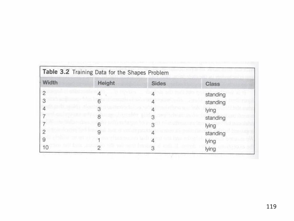
• The book illustrates the idea with the concept of geometric figures standing up or lying down, as shown in Figure 3.9 on the following overhead

• Comparing attributes with fixed values might work for a given data set

• However, in general, the problem involves comparing width and height attributes of instances

96

Figure 3.9

97

Dealing with Attribute-Attribute Comparisons

• It may be computationally expensive for an algorithm to compare instance attributes

• Preprocessing data for input may include hardcoding the comparison as an attribute itself

• Note how this implies that the user already understands the relationship between attributes in the first place

98

Inductive Logic Programming

• This subsection is really just about terminology

• The tasks getHeight() and getWidth() could be functionalized

• Composite geometric figures could be defined

99

• Recursive rules could be defined for determining whether composite figures were lying or standing

• This branch of data mining is called inductive logic programming

• It will not be pursued further

100

3.5 Instance-Based Representation

• Recall that the general topic of this chapter is “output” of data mining

• Recall that in the first subsection the output was a table of the data in organized, or sorted form

• The underlying idea is that the data set is itself, somehow, the result of the mining

101

• The scenario now is that you don’t start with an accumulated training set (table) of data

• Instead, data items arrive one-by-one, and you mine the data, i.e., try to classify it, for example, on the fly

• The end result should be a data set that where each item has been assigned to a class

102

• There is a category of data mining algorithms that is based on the concept of a nearest neighbor

• For each new instance that arrives, find its nearest neighbor in the set and classify it accordingly

103

• In practice, these kinds of algorithms usually find the k nearest neighbors

• They include a scheme for picking the class, like the majority class of the k nearest neighbors

104

Prerequisites for Mining in this Way

• You need to define distance in the space of the n attributes of the instances

• Potentially you need to normalize or weight the individual attributes

• In general, you need to know which attributes are important in the problem domain

• In short, the existing data set should already contain correct classifications

105

• Comparing a new instance with all existing instances is generally too expensive

• This is how come the subset of the k nearest existing neighbors is used when classifying new instances

106

Instance-Based Methods and Structural Representation

• Instance-based methods don’t immediately appear to provide a structural representation, like a rule set

• However, taken together, the different parts of the process form a representation

• The training subset, distance metric, and nearest neighbor rule define boundaries in n-space between instances

107

• In effect, this forms a structural representation analogous to something seen before:

• You fall on one side or the other of a decision boundary in space

108

• Figure 3.10, on the following overhead, illustrates some related ideas

• They are discussed after the figure is presented

109

110

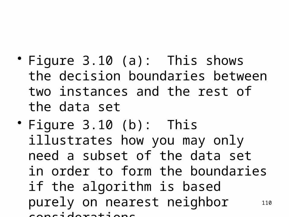
• Figure 3.10 (a): This shows the decision boundaries between two instances and the rest of the data set

• Figure 3.10 (b): This illustrates how you may only need a subset of the data set in order to form the boundaries if the algorithm is based purely on nearest neighbor considerations

111

• Figure 3.10 (c): This shows that in practice the classification neighborhoods will be simplified to rectangular areas in space

• Figure 3.10 (d): This illustrates the idea that you can have donut shaped classes, with one class’s instances completely contained within another’s

112

3.6 Clusters

• Clustering is not the classification of individual instances

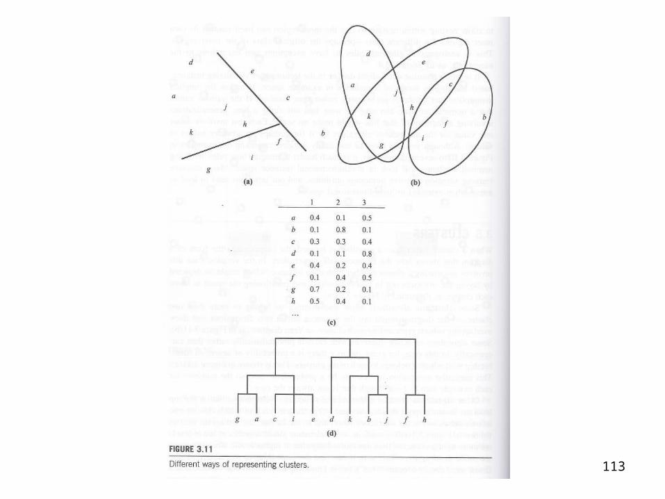
• It is the partitioning of the space• The book illustrates the ideas with Figure

3.11, shown on the following overhead• This is followed by brief explanatory

comments

113

114

• Figure 3.11 (a): This shows mutually exclusive partitions or classes

• Figure 3.11 (b): This shows that instances may be classified in >1 cluster

• Figure 3.11 (c): This shows that the assignment of an instance to a cluster may be probabilistic

• Figure 3.11 (d): A dendrogram is a technique for showing hierarchical relationships among clusters

115

The End

116

• You can ignore the following overheads• They’re just stored here for future

reference• They were not included in the current

version of the presentation of chapter 3

117

118

119