1 data analysis with matlab - elsevier · data analysis with matlab 1.1 why matlab?1 1.2 getting...

1 Data analysis with MatLab

1.1 Why MatLab? 1

1.2 Getting started with MatLab 3

1.3 Getting organized 3

1.4 Navigating folders 4

1.5 Simple arithmetic and algebra 5

1.6 Vectors and matrices 7

1.7 Multiplication of vectors of matrices 7

1.8 Element access 8

1.9 To loop or not to loop 9

1.10 The matrix inverse 11

1.11 Loading data from a file 11

1.12 Plotting data 12

1.13 Saving data to a file 13

1.14 Some advice on writing scripts 13

Problems 15

1.1 Why MatLab?

Data analysis requires computer-based computation. While a person can learn much

of the theory of data analysis by working through short pencil-and-paper examples, he

or she cannot become proficient in the practice of data analysis that way—for reasons

both good and bad. Real datasets, which are almost always too large to handle man-

ually, are inherently richer and more interesting than stripped-down examples. They

have more to offer, but an expanded skill set is required to successfully tackle them. In

particular, a new kind of judgment is required for selecting the analysis technique that

is right for the problem at hand. These are good reasons. Unfortunately, the practice of

data analysis is littered with bad reasons, too, most of which are related to the very

steep learning curve associated with using computers. Many practitioners of data anal-

ysis find that they spend rather too many frustrating hours solving computer-related

problems that have very little to do with data analysis, per se. That’s bad, especially ina classroom setting where time is limited and where frustration gets in the way of

learning.

One approach to dealing with this problem is to conduct all the data analysis within

a single software environment—to limit the damage. Frustrating software problems

will still arise, but fewer than if data were being shuffled between several different

Environmental Data Analysis with MatLab. DOI: 10.1016/B978-0-12-391886-4.00001-5

Copyright # 2012 by Elsevier Inc. All rights reserved.

environments. Furthermore, in a group setting such as a classroom, the memory and

experience of the group can help individuals solve commonly encountered problems.

The trick is to select a single software environment that is capable of supporting realdata analysis.

The key decision is whether to go with a spreadsheet or a scripting language-type

software environment. Both are viable environments for computer-based data analy-

sis. Stable implementations of both are available for most types of computers from

commercial software developers at relatively modest prices (and especially for those

eligible for student discounts). Both provide support for the data analysis itself, as well

as associated tasks such as loading and writing data to and from files and plotting them

on graphs. Spreadsheets and scripting languages are radically different in approach,

and each has advantages and disadvantages.

In a spreadsheet-type environment, typified byMicrosoft Excel, data are presentedas one or more tables. Data are manipulated by selecting the rows and columns of a

table and operating on them with functions selected from a menu and with formulas

entered into the cells of the table itself. The immediacy of a spreadsheet is both its

greatest advantage and its weakness. You see the data and all the intermediate results

as you manipulate the table. You are, in a sense, touching the data, which gives you a

great sense of what the data are like. More of a problem, however, is keeping track of

what you did in a spreadsheet-type environment, as is transferring useful procedures

from one spreadsheet-based dataset to another.

In a scripting language, typified by The MathWorks MatLab, data are presented

as one or more named variables (in the same sense that the “c” and “d” in the formula

c¼ pd are named variables). Data are manipulated by typing formulas that create new

variables from old ones and by running scripts, that is, sequences of formulas stored in

a file. Much of data analysis is simply the application of well-known formulas to novel

data, so the great advantage of this approach is that the formulas that you type usually

have a strong similarity to those printed in a textbook. Furthermore, scripts provide a

way of both documenting the sequence of formulas used to analyze a particular dataset

and transferring the overall data analysis procedure from one dataset to another. The

main disadvantage of a scripting language environment is that it hides the data within

the variable—not absolutely, but a conscious effort is nonetheless needed to display it

as a table or as a graph. Things can go badly wrong in a script-based data analysis

scheme without the practitioner being aware of it. Another disadvantage is that the

parallel between the syntax of the scripting language and the syntax of standard math-

ematical notation is nowhere near perfect. One needs to learn to translate one into the

other.

While both spreadsheets and scripting languages have pros and cons, our opinion isthat, on balance, a scripting language wins out, at least for the data analysis scenarios

encountered in Environmental Science. In our experience, these scenarios often re-

quire a long sequence of data manipulation steps before a final result is achieved.

Here, the self-documenting aspect of the script is paramount. It allows the practitioner

to review the data processing procedure both as it is being developed and years after it

has been completed. It provides a way of communicating what you did, a process thatis at the heart of science.

2 Environmental Data Analysis with MatLab

We have chosen MatLab, a commercial software product of The MathWorks, Inc.as our preferred software environment for several reasons, some having to do with its

designs and others more practical. The most persuasive design reason is that its syntax

fully supports both linear algebra and complex arithmetic, both of which are important

in data analysis. Practical considerations include the following: it is a long-lived and

stable product, available since the mid 1980s; implementations are available for most

commonly used types of computers; its price, especially for students, is fairly modest;

and it is widely used, at least in university settings.

1.2 Getting started with MatLab

We cannot walk you through the installation of MatLab, for procedures vary from

computer to computer and quickly become outdated, anyway. Furthermore, we will

avoid discussion of the appearance of MatLab on your computer screen, because

its Graphical User Interface has evolved significantly over the years and can be

expected to continue to do so. We will assume that you have successfully installed

MatLab and that you can identify the Command Window, the place where MatLabformula and commands are typed.

You might try typing

date

in this window. If MatLab responds by displaying the current date, you’re on track!

All the MatLab commands that we use are in MatLab scripts that are provided as

a companion to this book. This one is named eda01_01 and is in a MatLab script

file (m-file, for short) named eda01_01.m (conventionally, m-files have file names

that end with “.m”). In this case, the script is pretty boring, as it contains just this

one command, date, together with a couple of comment lines (which start with the

character “%”):

% eda01_01

% displays the current date

date (MatLab eda01_01)

After you installMatLab, you should copy the eda folder, provided with this book, to

your computer’s file system. Put it in some convenient and easy-to-remember place

that you are not going to accidentally delete!

1.3 Getting organized

Files proliferate at an astonishing rate, even in the most trivial data management pro-

ject. You start with a file of data, but then write m-scripts, each of which has its own

file. You will usually output final results of the data analysis to a file, and you may

well output intermediate results to files, too. You will probably have files containing

graphs and files containing notes as well. Furthermore, you might decide to analyze

Data analysis with MatLab 3

your data in several different ways, so you may have several versions of some of

these files.

A practitioner of data analysis may find that a little organization up front saves

quite a bit of confusion down the line.

As data analysis scenarios vary widely, there can be no set rule regarding organi-

zation of the files associated with them. The goal should simply be to create a system

of folders (directories), subfolders (sub-directories), and file names that are suffi-

ciently systematic so that files can be located easily and they are not confused with

one another. Predictability in both the pattern of filenames and in the arrangement

of folders and subfolders is an extremely important part of the design.

By way of example, the files associated with this book are in a three-tiered folder/

subfolder structure modeled on the chapter and section format of the book itself

(Figure 1.1). Most of the files, such as the m-files, are in the chapter folders. However,

some chapters have longish case studies that use a large number of files, and in those

instances, section folders are used. Folder and file names are systematic. The chapter

folder names are always of the form chNN, where NN is the chapter number. The section

folder names are always of the form secNN_MM, where NN is the chapter number and MM

is the section number. We have chosen to use leading zeros in the naming scheme

(for example, ch01) so that filenames appear in the correct order when they are sorted

alphabetically (as when listing the contents of a folder).

1.4 Navigating folders

The MatLab command window supports a number of commands that enable you to

navigate from folder to folder, list the contents of folders, and so on. For example,

when you type

pwd

(for “print working directory”) in the Command Window, MatLab responds by dis-

playing the name of the current folder. Initially, this is almost invariably the wrong

Main folder Chapter folders Chapter files andsection folders

Section files

eda ch01

ch02 file

file

ch03. . .

. . . sec02_01 file

file. . .file. . .

Figure 1.1 Folder (directory) structure used for the files accompanying this book.


folder, so you will need to cd (for “change directory”) to the folder where you want to

be—the ch01 folder in this case. The pathname will, of course, depend on where you

copied the eda folder, but will end in eda/ch01. On our computer, typing

cd c:/menke/docs/eda/ch01

does the trick. If you have spaces in your pathname, just surround it with single quotes:

cd ‘c:/menke/my docs/eda/ch01’

You can check if you are in the right folder by typing pwd again. Once in the ch01

folder, typing

eda01_01

will run the eda01_01 m-script, which displays the current date. You can move to the

folder above the current one by typing

cd ..

and to one below it by giving just the folder name. For example, if you are in the eda

folder you can move to the ch01 folder by typing

cd ch01

Finally, the command dir (for “directory”), lists the files and subfolders in the current

directory.

dir (MatLab eda01_02)

1.5 Simple arithmetic and algebra

The MatLab commands for simple arithmetic and algebra closely parallel standard

mathematical notation. For instance, the command sequence

a ¼ 3.5;

b ¼ 4.1;

c ¼ aþb;

c (MatLab eda01_03)

evaluates the formula c¼ aþ b for the case a¼ 3.5 and b¼ 4.1 to obtain c¼ 7.6. Only

the semicolons require explanation. By default, MatLab displays the value of every

formula typed into the CommandWindow. A semicolon at the end of the formula sup-

presses the display. Hence, the first three lines, which end with semicolons, are eval-

uated but not displayed. Only the final line, which lacks the semi-colon, causes

MatLab to print the final result, c.

A perceptive reader might have noticed that the m-script could have been made

shorter by one line, simply by omitting the semicolon in the formula, c¼aþb.That is,

a ¼ 3.5;

b ¼ 4.1;

c ¼ aþb


However, we recommend against such cleverness. The reason is that many interme-

diate results will need to be temporarily displayed and then un-displayed in the process

of developing and debugging a long m-script. When this is accomplished by adding

and then deleting the semicolon at the end of a functioning—and important—formula

in the script, the formula can be inadvertently damaged by deleting one or more extra

characters. Editing a line of the code that has no function other than displaying a value

is safer.Note thatMatLab variables are static, meaning that they persist inMatLab’s Work-

space until you explicitly delete them or exit the program. Variables created by one

script can be used by subsequent scripts. At any time, the value of a variable can be

examined, either by displaying it in the Command Window (as we have done above)

or by using the spreadsheet-like display tools available throughMatLab’sWorkspace

Window. The persistence ofMatLab variables can sometimes lead to scripting errors,

as described in Note 1.1.

The four commands discussed above can be run as a unit by typing eda01_03. Now

open the m-file eda01_03 inMatLab, using the File/Open menu.MatLabwill bring upa text-editor type window. First save it as a new file, say myeda01_03, edit it in some

simple way, say by changing the 3.5 to 4.5, save the edited file, and run it by typing

myeda01_03 in the CommandWindow. The value of c that is displayed will have chan-

ged appropriately.

A somewhat more complicated MatLab formula is

c ¼ffiffiffiffiffiffiffiffiffiffiffiffiffiffiffia2 þ b2

pwith a ¼ 3 and b ¼ 4

a ¼ 3;

b ¼ 4;

c ¼ sqrt(a^2 þ b^2);

c (MatLab eda01_04)

Note that the MatLab syntax for a2 is a^2 and that the square root is computed using

the function, sqrt(). This is an example ofMatLab’s syntax differing from standard

mathematical notation.

A final example is

c ¼ sinnpðx� x0Þ

Lwith n ¼ 2, x ¼ 3, x0 ¼ 1, L ¼ 5

n ¼ 2; x ¼ 3; x0 ¼ 1; L ¼ 5;

c ¼ sin(n*pi*(x�x0)/L);

c (MatLab eda01_05)

Note that several formulas separated by semicolons can be typed on the same line.

Variables, such as x0 and pi above, can have names consisting of more than one char-

acter, and can contain numerals as well as letters (although they must start with a

letter). MatLab has a variety of predefined mathematical constants, including pi,

which is the usual mathematical constant, p.


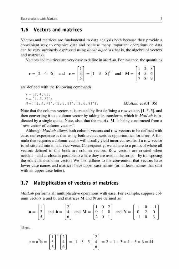
1.6 Vectors and matrices

Vectors and matrices are fundamental to data analysis both because they provide a

convenient way to organize data and because many important operations on data

can be very succinctly expressed using linear algebra (that is, the algebra of vectors

and matrices).

Vectors and matrices are very easy to define inMatLab. For instance, the quantities

r ¼ ½ 2 4 6 � and c ¼1

3

5

24

35 ¼ ½ 1 3 5 �T and M ¼

1 2 3

4 5 6

7 8 9

24

35

are defined with the following commands:

r ¼ [2, 4, 6];

c ¼ [1, 2, 3]’;

M ¼[ [1, 4, 7]’, [2, 5, 8]’, [3, 6, 9]’]; (MatLab eda01_06)

Note that the column-vector, c, is created by first defining a row vector, [1, 3, 5], and

then converting it to a column vector by taking its transform, which in MatLab is in-

dicated by a single quote. Note, also, that the matrix, M, is being constructed from a

“row vector of column vectors”.

Although MatLab allows both column-vectors and row-vectors to be defined with

ease, our experience is that using both creates serious opportunities for error. A for-

mula that requires a column-vector will usually yield incorrect results if a row-vector

is substituted into it, and vice-versa. Consequently, we adhere to a protocol where all

vectors defined in this book are column vectors. Row vectors are created when

needed—and as close as possible to where they are used in the script—by transposing

the equivalent column vector. We also adhere to the convention that vectors have

lower-case names and matrices have upper-case names (or, at least, names that start

with an upper-case letter).

1.7 Multiplication of vectors of matrices

MatLab performs all multiplicative operations with ease. For example, suppose col-

umn vectors a and b, and matrices M and N are defined as

a ¼1

3

5

24

35 and b ¼

2

4

6

24

35 and M ¼

1 0 2

0 1 0

2 0 1

24

35 and N ¼

1 0 �1

0 2 0

�1 0 3

24

35

Then,

s ¼ aTb ¼1

3

5

24

35T

2

4

6

24

35 ¼ ½ 1 3 5 �

2

4

6

24

35 ¼ 2� 1þ 3� 4þ 5� 6 ¼ 44


T ¼ abT ¼1

3

5

24

35 2

4

6

24

35T

¼2� 1 4� 1 6� 1

2� 3 4� 3 6� 3

2� 5 4� 5 6� 5

24

35 ¼

2 4 6

6 12 18

10 20 30

24

35

c ¼ Ma ¼1 0 2

0 1 0

2 0 1

24

35 1

3

5

24

35 ¼

1� 1 þ 0� 3 þ 2� 5

0� 1 þ 1� 3 þ 0� 5

2� 1 þ 0� 3 þ 1� 5

24

35 ¼

11

3

7

24

35

P ¼ MN ¼1 0 2

0 1 0

2 0 1

24

35 1 0 �1

0 2 0

�1 0 3

24

35 ¼

�1 0 5

0 2 0

1 0 1

24

35

corresponds to

s ¼ a0*b;T ¼ a*b0;c ¼ M*a;

P ¼ M*N; (MatLab eda01_07)

In MatLab, standard vector and matrix multiplication is performed just by using the

normal multiplications sign, * (the asterisk). There are cases, however, where one

needs to violate these rules and multiply the quantities element-wise (for example,

create a vector, d, with elements di ¼ aibi). MatLab provides a special element-wise

version of the multiplication sign, denoted.* (a period followed by an asterisk):

d ¼ a.*b; (MatLab eda01_07)

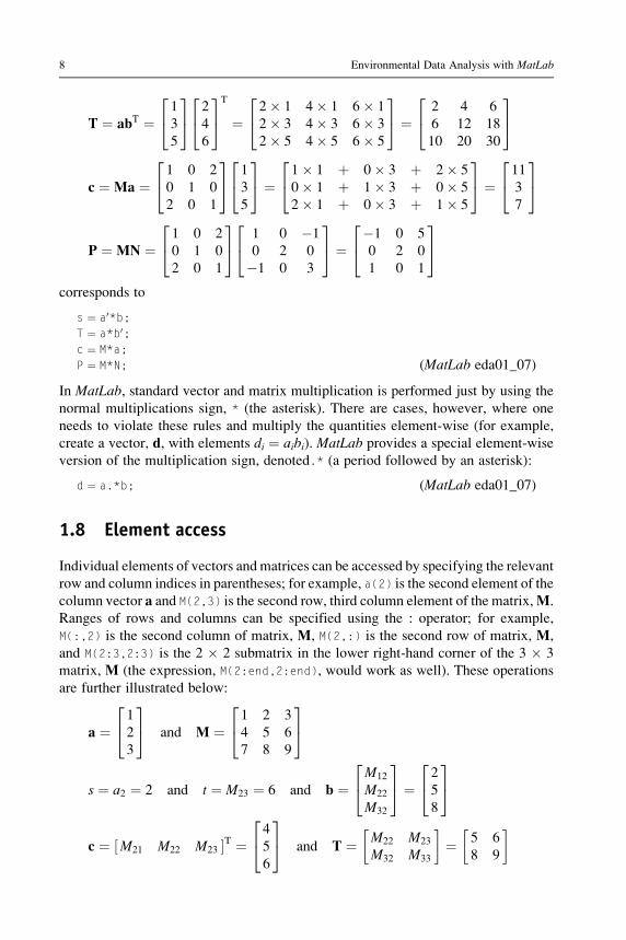
1.8 Element access

Individual elements of vectors and matrices can be accessed by specifying the relevant

row and column indices in parentheses; for example, a(2) is the second element of the

column vector a and M(2,3) is the second row, third column element of the matrix,M.

Ranges of rows and columns can be specified using the : operator; for example,

M(:,2) is the second column of matrix, M, M(2,:) is the second row of matrix, M,

and M(2:3,2:3) is the 2 � 2 submatrix in the lower right-hand corner of the 3 � 3

matrix, M (the expression, M(2:end,2:end), would work as well). These operations

are further illustrated below:

a ¼1

2

3

24

35 and M ¼

1 2 3

4 5 6

7 8 9

24

35

s ¼ a2 ¼ 2 and t ¼ M23 ¼ 6 and b ¼M12

M22

M32

24

35 ¼

2

5

8

24

35

c ¼ ½M21 M22 M23 �T ¼4

5

6

24

35 and T ¼ M22 M23

M32 M33

� �¼ 5 6

8 9

� �


correspond to:

s ¼ a(2);

t ¼ M(2,3);

b ¼ M(:,2);

c ¼ M(2,:)’;

T ¼ M(2:3,2:3); (MatLab eda01_08)

The colon notion can be used in other contexts as well. For instance, [1:4] is the row

vector [1, 2, 3, 4]. The syntax, 1:4, which omits the square brackets, works fine in

MatLab. However, we usually use square brackets, as they draw attention to the pres-

ence of a vector. Finally, we note that two colons can be used in sequence to indicate

the spacing of elements in the resulting vector. For example, the expression [1:2:9] is

the row vector [1, 3, 5, 7, 9] and the expression [10:�1:1] is a row vector whose el-

ements are in the reverse order from [10:1].

1.9 To loop or not to loop

MatLab provides a looping mechanism, the for command, which can be useful when

the need arises to sequentially access the elements of vectors and matrices. Thus, for

example,

M ¼ [ [1, 4, 7]’, [2, 5, 8]’, [3, 6, 9]’ ];

for i ¼ [1:3]

a(i) ¼ M(i,i);

end (MatLab eda01_09)

executes the a(i) ¼ M(i,i)formula three times, each time with a different value of i

(in this case, i¼ 1, i¼ 2, and i¼ 3). The net effect is to copy the diagonal elements of

the matrixM to the vector, a, that is, ai¼Mii. Note that the end statement indicates the

position of the bottom of the loop. Subsequent commands are not part of the loop and

are executed only once.

Loops can be nested; that is, one loop can be inside another. Such an arrangement is

necessary for accessing all the elements of a matrix in sequence. For example,

M ¼ [ [1, 4, 7]’, [2, 5, 8]’, [3, 6, 9]’];

for i ¼ [1:3]

for j ¼ [1:3]

N(i,4�j) ¼ M(i,j);

end


copies the elements of the matrix, M, to the matrix, N, but reverses the order of the

elements in each row; that is, Ni,j ¼Mi,4�j. Loops are especially useful in conjunction

with conditional commands. For example

a ¼ [ 1, 2, 1, 4, 3, 2, 6, 4, 9, 2, 1, 4 ]’;

for i ¼ [1:12]


if ( a(i) >¼ 6 )

b(i) ¼ 6;

else

b(i) ¼ a(i);

end


sets bi¼ ai if ai< 6 and sets bi¼ 6 otherwise (a process called clipping a vector, for itlops off parts of the vector that are larger than 6).

A purist might point out thatMatLab syntax is so flexible that for loops are almost

never really necessary. In fact, all three examples, above, can be computed with one-

line formulas that omit for loops:

a ¼ diag(M);

N ¼ fliplr(M);

b ¼ a.*(a<6)þ6.*(a>¼6); (MatLab eda01_12)

The first two formulas are quite simple, but rely on theMatLab functions diag() andfliplr()whose existence we have not heretofore mentioned. One of the problems of

a script-based environment is that learning the complete syntax of the scripting lan-

guage can be pretty daunting. Writing a long script, such as one containing a for

loop, will often be faster than searching through MatLab help files for a predefined

function that implements the desired functionality in a single line of the script. The

third formula points out a different problem: MatLab syntax is often pretty inscru-

table. In this case, the expression (a<6) creates a column-vector of ones and zeros,

depending on whether a given element of a is less-than or greater-than-or-equal-to 6.

Element-wise multiplication is then used to create a vector a.*(a<6) whose ele-

ments are either ai or 0. Similarly, 6.*(a>¼6) is a vector whose elements are either

0 or 6. Their sum is a vector whose elements are either ai or 6, depending on whetherai is less-than or greater-than-or-equal-to 6. That’s pretty complicated!

Because MatLab’s syntax is so powerful, the same functionality can often be

achieved in several different ways. Thus, for example, the commands

b ¼ a;

b(find(a>6)) ¼ 6; (MatLab eda01_12)

will also clip the elements of the vector. The find() function returns a column-

vector of the indices of the vector, a, that match the condition, and then that list is

used to reset just those elements of b to 6, leaving the other elements unchanged.

When deciding between alternative ways of implementing a given functionality,

you should always choose the one which you find clearest. Scripts that are terse or

even computationally efficient are not necessarily a virtue, especially if they are dif-

ficult to debug. You should avoid creating formulas that are so inscrutable that you are

not sure whether they will function correctly. Of course, the degree of inscrutability of

any given formula will depend on your level of familiarity withMatLab. Your reper-toire of techniques will grow as you become more practiced.


1.10 The matrix inverse

Recall that the matrix inverse is defined only for square matrices, and that it has the

following properties:

A�1A ¼ AA�1 ¼ I ð1:1Þ

Here, I is the identity matrix, that is, a matrix with ones on its main diagonal and zeros

elsewhere. In MatLab, the matrix inverse is computed as

B ¼ inv(A); (MatLab eda01_13)

In many of the formulas of data analysis, the matrix inverse either premultiplies or

postmultiplies other quantities; for instance,

c ¼ A�1b and D ¼ BA�1

These cases do not actually require the explicit calculation of A-1; just the combina-

tions A�1b and BA�1, which are computationally simpler are sufficient. MatLabprovides generalizations of the division operator that implements these two cases:

c ¼ A\b;

D ¼ B/A; (MatLab eda01_14)

1.11 Loading data from a file

MatLab can read and write files with a variety of formats, but we start here with the

simplest and most common one, the text file.

As an example, we load a hydrological dataset of stream flow from the Neuse River

near Goldsboro NC. Our recommendation is that you always keep a file of notes about

any dataset that you work with, and that these notes include information on where you

obtained the dataset and any modifications that you subsequently made to it. Bill

Menke provides the following notes for this one (Figure 1.2):

I downloaded stream flow data from the US Geological Survey’s National WaterInformatiuon Center for the Neuse River near Goldboro NC for the time period,01/01/1974-12/31/1985. These data are in the file, neuse.txt. It contains two col-umns of data, time (in days starting on January 1, 1974) and discharge (in cubic feetper second, cfs). The data set contains 4383 rows of data. I also saved informationabout the data in the file neuse_header.txt.

We reproduce the first few lines of neuse.txt, here:

1 1450

2 2490

3 3250

. . .. . . ..


The data is read into MatLab as follows:

D ¼ load(‘neuse.txt’);

t ¼ D(:,1);

d ¼ D(:,2); (MatLab eda01_15)

The load() function reads the data into a 4383 � 2 array, D. Note that the filename,

neuse.txt, needs to be surrounded by single quotes to indicate that it is a characterstring and not a variable name. The subsequent two lines break outD into two separate

column-vectors, t, of time and d, of discharge. Strictly speaking, this step is not nec-

essary, but our opinion is that fewer mistakes will be made if each of the different

variables in the dataset has its own name.

1.12 Plotting data

One of the best things to do after loading a new dataset is to make a quick plot of it, just

to get a sense of what it looks like. Such plots are very easily created in MatLab:

plot(t,d);

The resulting plot is quite functional, but lacks some graphical niceties such as labeled

axes and a title. These deficiencies are easy to correct:

set(gca,‘LineWidth’,2);

plot(t,d,‘k�’,‘LineWidth’,2);

500

2.5´104

1000 1500 2000 2500 3000 3500 4000 4500

2

1.5

1

0.5

00

Figure 1.2 Preliminary plot of the Neuse River discharge dataset. MatLab script eda01_05.


title(‘Neuse River Hydrograph’);

xlabel(‘time in days’);

ylabel(‘discharge in cfs’); (MatLab eda01_16)

The set command resets the line width of the axes, to make them easier to see. Several

new arguments have been added to the plot() function. The ‘k�‘ changes the plot

color from its default value (a blue line, at least on our computer) to a black line.

The ‘LineWidth’, 2 makes the line thicker (which is important if you print the plot

to paper). A quick review of the plot indicates that the Neuse River discharge has some

interesting properties, such as pattern of highs and lows that repeat every few hundred

days. We will discuss it more extensively in Chapter 2.

1.13 Saving data to a file

Data is saved to a to text file in a process that is more or less the reverse of the one used

to read it. Suppose, for instance, that we want a version of neuse.txt that contains dis-

charge in the metric units of m3/s. After looking up the conversion factor, f¼ 35.3146,

between cubic feet and cubic meters, we perform the conversion and write the data to a

new file:

f ¼ 35.3146;

dm ¼ d/f;

Dm(:,1) ¼ t;

Dm(:,2) ¼ dm;

dlmwrite(‘neuse_metric.txt’,Dm,’\t’); (MatLab eda01_17)

The function dlmwrite() (for “delimited write”) writes the matrix, Dm, to the file neu-

se_metric.txt, putting a tab character (which in MatLab is represented with

the symbol, \t)between the columns as a delimiter. Note that the filename and the

delimiter are quoted; they are character strings.

1.14 Some advice on writing scripts

Practices that reduce the likelihood of scripting mistakes (“bugs”) are almost always

worthwhile, even though they may seem to slow you down a bit. They save time in the

long run, as you will spend much less time debugging your scripts.

1.14.1 Think before you type

Think about what you want to do before starting to type in a script. Block out the nec-

essary steps on a piece of scratch paper.Without some forethought, you can type for an

hour and then realize that what you have been doing makes no sense at all.


1.14.2 Name variables consistently

MatLab automatically creates a new variable whenever you type a new variable name.

That is convenient, but it means that a misspelled variable becomes a new variable.

For instance, if you begin calling a quantity xmin but accidentally switch to minx half-

way through, you will unknowingly have two variables in your script, and it will not

function correctly. Do not tempt fate by creating two variables, such as xmin and miny,

with an inconsistent naming pattern.

1.14.3 Save old scripts

Cannibalize an old script to make a new one, but keep a copy of the old one too, and

make sure that the names are sufficiently different so that you will not confuse them

with each other.

1.14.4 Cut and paste sparingly

Cutting and pasting segments of code from one script to another, tempting though it

may be, is especially prone to error, particularly when variable names need to be chan-

ged. Read through the cut-and-pasted material carefully, to make sure that all neces-

sary changes have been made.

1.14.5 Start small

Build scripts in small sections. Test each section thoroughly before going into the

next. Check intermediate results, either by displaying variables to the CommandWin-

dow, examining them with the spreadsheet tool in theWorkspace Window, or by plot-

ting them, to ensure that they look right.

1.14.6 Test your scripts

Build test datasets with known properties to test whether or not your scripts give the

right answers. Test a script on a small, simple dataset before running it on large com-

plicated datasets.

1.14.7 Comment your scripts

Use comments to communicate the big picture, not the minutia. Consider the two

scripts in Figure 1.3. Which of the two styles of commenting code do you suppose

will make a script easier to understand 2 years down the line?

1.14.8 Don’t be too clever

An inscrutable script is very prone to error.


Problems

1.1 Write MatLab scripts to evaluate the following equations:

ðAÞ y ¼ ax2 þ bxþ c with a ¼ 2, b ¼ 4, c ¼ 8, x ¼ 3:5

ðBÞ p ¼ p0 expð�cxÞ with p0 ¼ 1:6, c ¼ 4, x ¼ 3:5

ðCÞ z ¼ h siny with h ¼ 4, y ¼ 31�

ðDÞ v ¼ phr2 with h ¼ 6:9, r ¼ 3:71.2 Write aMatLab script that defines a column vector, a, of length N¼ 12 whose elements are

the number of days in the 12 months of the year, for a nonleap year. Create a similar column

vector, b, for a leap year. Then merge a and b together into an N �M ¼ 12 � 2 matrix, C.

1.3 Write a MatLab script that solves the following linear equation, y ¼ M x, for x:

M ¼1 �1 0 0

0 1 �1 0

0 0 1 �1

0 0 0 1

2664

3775 and y ¼

1

2

3

5

2664

3775

You may find useful theMatLab function zeros(N, N), which creates a N � Nmatrix of

zeros. Be sure to check that your x solves the original equation.

1.4 Create a 50� 50 version of theM, above. One possibility is to use a for loop. Another is to

use the MatLab function toeplitz(),as M has the form of a Toeplitz matrix, that is, a

matrix with constant diagonals. Type helptoeplitz in the CommandWindow for details

on how this function is called.

1.5 Rivers always flow downstream. Write a MatLab script to check that none of the Neuse

River discharge data is negative.

B esaCA esaC

% Evaluate Normal distribution CI=inv(C); % take inverse of C % with mean dbar and covariance, C

norm=1/(2*pi*sqrt(det(C))); % compute norm

CI=inv(C);1/(2* i* t(d t(C)))

Pp=zeros(L,L);% l inorm= p sqr e ;

Pp=zeros(L L); oop over for i = [1:L],

for i = [1:L] =

% loop over jfor j = [1:L]dd [d1(i) d1b d2(j) d2b ]'

for j = [1:L]% dd i 2 t= i)- ar, - ar ;

Pp(i j)=norm*exp( −0 5 * dd' * CI* dd ); is a -vector

dd = [d1(i)-d1bar d2(j)-d2bar]';, . end

= i) , % compute exponential

;)dd *IC * 'dd* 5.0− (pxe*mron=)j,i(pPdneden

end

Figure 1.3 The same script, commented in two different ways.


1 data analysis with matlab - elsevier · data analysis with matlab 1.1 why matlab?1 1.2 getting...

Documents