1 continuous random variables a discrete random variable is one that can take only a finite set of...

1

CONTINUOUS RANDOM VARIABLES

A discrete random variable is one that can take only a finite set of values. The sum of the numbers when two dice are thrown is an example.

6

__

36

5

__

36

4

__

36

3

__

36

2

__

36

2

__

36

3

__

36

5

__

36

4

__

36

probability

2 3 4 5 6 7 8 9 10 11 12 X

1

36

1

36

Each value has associated with it a finite probability, which you can think of as a ‘packet’ of probability. The packets sum to unity because the variable must take one of the values.

2


6

__

36

5

__

36

4

__

36

3

__

36

2

__

36

2

__

36

3

__

36

5

__

36

4

__

36

probability

2 3 4 5 6 7 8 9 10 11 12 X

1

36

1

36

55 60 70 75 X65

height

However, most random variables encountered in econometrics are continuous. They can take any one of an infinite set of values defined over a range (or possibly, ranges).

3


As a simple example, take the temperature in a room. We will assume that it can be anywhere from 55 to 75 degrees Fahrenheit with equal probability within the range.

4


55 60 70 75 X65

height

In the case of a continuous random variable, the probability of it being equal to a given finite value (for example, temperature equal to 55.473927) is always infinitesimal.

5


55 60 70 75 X65

height

For this reason, you can only talk about the probability of a continuous random variable lying between two given values. The probability is represented graphically as an area.

6


55 60 70 75 X65

height

7

55 60 70 75 X65

height

For example, you could measure the probability of the temperature being between 55 and 56, both measured exactly.

56


8

55 60 70 75 X65

height

56

Given that the temperature lies anywhere between 55 and 75 with equal probability, the probability of it lying between 55 and 56 must be 0.05.

0.05


9

55 60 70 75 X65

height

56

0.05

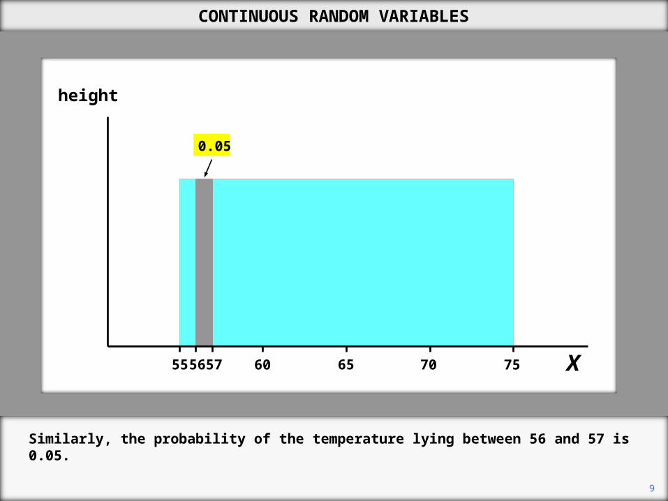
Similarly, the probability of the temperature lying between 56 and 57 is 0.05.

57


10

55 60 70 75 X65

height

56

0.05

5758

And similarly for all the other one-degree intervals within the range.


11

55 60 70 75 X65

height

565758

0.05

The probability per unit interval is 0.05 and accordingly the area of the rectangle representing the probability of the temperature lying in any given unit interval is 0.05.


12

55 60 70 75 X65

height

565758

0.05

The probability per unit interval is called the probability density and it is equal to the height of the unit-interval rectangle.


13

55 60 70 75 X65

height

565758

0.05

Mathematically, the probability density is written as a function of the variable, for example f(X). In this example, f(X) is 0.05 for 55 < X < 75 and it is zero elsewhere.

f(X) = 0.05 for 55 X 75f(X) = 0 for X < 55 and X > 75


14

55 60 70 75 X65565758

0.05

The vertical axis is given the label probability density, rather than height. f(X) is known as the probability density function and is shown graphically in the diagram as the thick black line.

probabilitydensity

f(X)



15

55 60 70 75 X65

0.05

probabilitydensity

f(X)

Suppose that you wish to calculate the probability of the temperature lying between 65 and 70 degrees.



16

55 60 70 75 X65

0.05

probabilitydensity

f(X)

To do this, you should calculate the area under the probability density function between 65 and 70.



17

55 60 70 75 X65

0.05

probabilitydensity

f(X)

Typically you have to use the integral calculus to work out the area under a curve, but in this very simple example all you have to do is calculate the area of a rectangle.



18

55 60 70 75 X6556

0.05

probabilitydensity

f(X)

The height of the rectangle is 0.05 and its width is 5, so its area is 0.25.

0.25



19

70 75 X65

probabilitydensity

f(X)

Now suppose that the temperature can lie in the range 65 to 75 degrees, with uniformly decreasing probability as the temperature gets higher.


20

70 75 X65

probabilitydensity

f(X)

The total area of the triangle is unity because the probability of the temperature lying in the 65 to 75 range is unity. Since the base of the triangle is 10, its height must be 0.20.

0.20

0.15

0.10

0.05


21

70 75 X65

probabilitydensity

f(X)

0.20

0.15

0.10

0.05

In this example, the probability density function is a line of the form f(X) = b1 + b2X. To pass through the points (65, 0.20) and (75, 0), b1 must equal 1.50 and b2 must equal -0.02.

f(X) = 1.50 – 0.02X for 65 X 75f(X) = 0 for X < 65 and X > 75


22

70 75 X65

probabilitydensity

f(X)

0.20

0.15

0.10

0.05

Suppose that we are interested in finding the probability of the temperature lying between 65 and 70 degrees.



23

70 75 X65

probabilitydensity

f(X)

0.20

0.15

0.10

0.05

We could do this by evaluating the integral of the function over this range, but there is no need.



24

70 75 X65

probabilitydensity

f(X)

0.20

0.15

0.10

0.05

It is easy to show geometrically that the answer is 0.75. This completes the introduction to continuous random variables.



Copyright Christopher Dougherty 2012.

These slideshows may be downloaded by anyone, anywhere for personal use.

Subject to respect for copyright and, where appropriate, attribution, they may be

used as a resource for teaching an econometrics course. There is no need to

refer to the author.

The content of this slideshow comes from Section R.3 of C. Dougherty,

Introduction to Econometrics, fourth edition 2011, Oxford University Press.

Additional (free) resources for both students and instructors may be

downloaded from the OUP Online Resource Centre

http://www.oup.com/uk/orc/bin/9780199567089/.

Individuals studying econometrics on their own who feel that they might benefit

from participation in a formal course should consider the London School of

Economics summer school course

EC212 Introduction to Econometrics

http://www2.lse.ac.uk/study/summerSchools/summerSchool/Home.aspx

or the University of London International Programmes distance learning course

EC2020 Elements of Econometrics

www.londoninternational.ac.uk/lse.

2012.10.29

1 continuous random variables a discrete random variable is one that can take only a finite set of...

Documents