1 consumer behavior chapter 3. 2 theory of consumer behavior description of how consumers allocate...
TRANSCRIPT

1
Consumer Behavior
Chapter 3

2
theory of consumer behavior Description of how consumers allocate incomes among different goods and services to maximize their well-being.
Consumer behavior is best understood in three distinct
steps:
1. Consumer preferences
2. Budget constraints
3. Consumer choices
3
Consumer Preferences – Basic Assumptions
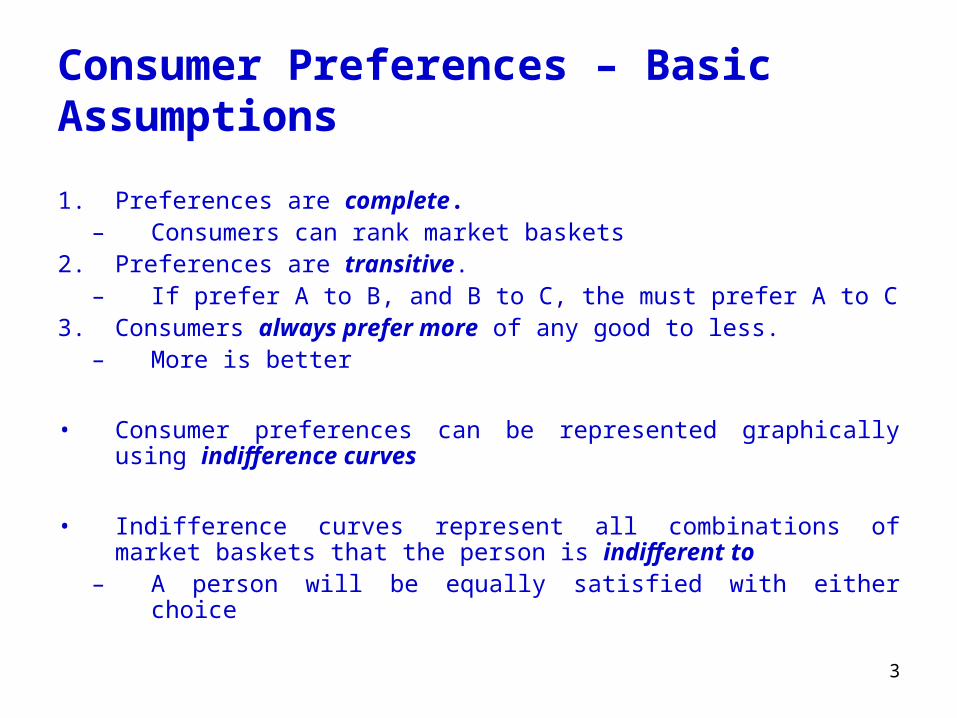
1. Preferences are complete.– Consumers can rank market baskets
2. Preferences are transitive.– If prefer A to B, and B to C, the must prefer A to C
3. Consumers always prefer more of any good to less.– More is better
• Consumer preferences can be represented graphically using indifference curves
• Indifference curves represent all combinations of market baskets that the person is indifferent to
– A person will be equally satisfied with either choice
4
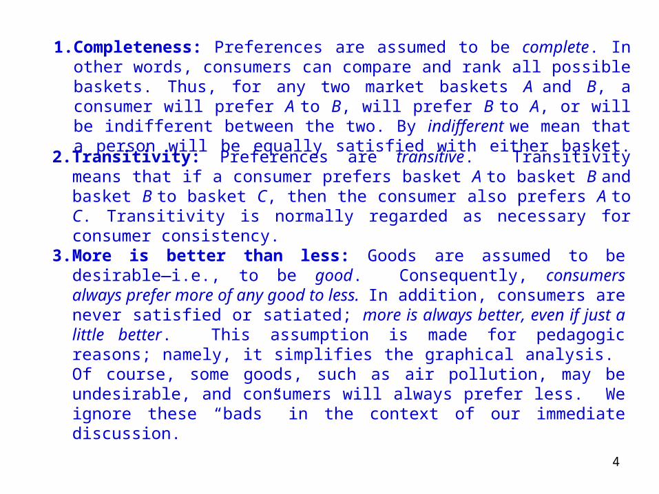
1.Completeness: Preferences are assumed to be complete. In other words, consumers can compare and rank all possible baskets. Thus, for any two market baskets A and B, a consumer will prefer A to B, will prefer B to A, or will be indifferent between the two. By indifferent we mean that a person will be equally satisfied with either basket.
2.Transitivity: Preferences are transitive. Transitivity means that if a consumer prefers basket A to basket B and basket B to basket C, then the consumer also prefers A to C. Transitivity is normally regarded as necessary for consumer consistency.
3.More is better than less: Goods are assumed to be desirable—i.e., to be good. Consequently, consumers always prefer more of any good to less. In addition, consumers are never satisfied or satiated; more is always better, even if just a little better. This assumption is made for pedagogic reasons; namely, it simplifies the graphical analysis. Of course, some goods, such as air pollution, may be undesirable, and consumers will always prefer less. We ignore these “bads” in the context of our immediate discussion.
5
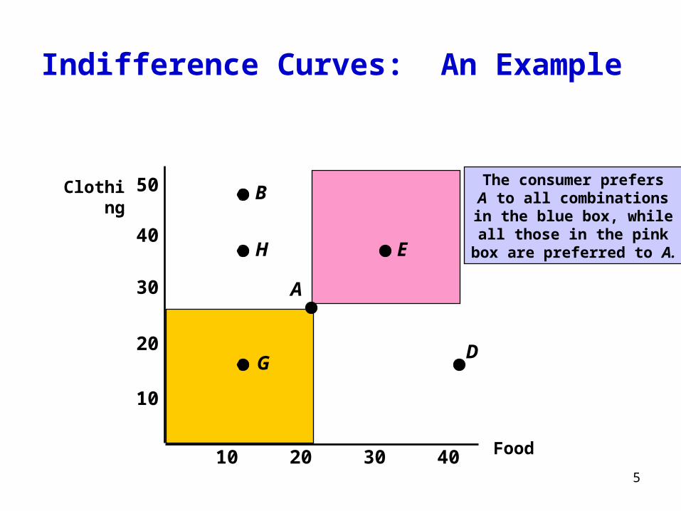
Indifference Curves: An Example
Food
10
20
30
40
10 20 30 40
Clothing
50
G
A
EH
B
D
The consumer prefersA to all combinationsin the blue box, whileall those in the pink
box are preferred to A.
6
• Points such as B & D have more of one good but less of another compared to A
– Need more information about consumer ranking
• Consumer may decide they are indifference between B, A and D
– We can then connect those points with an indifference curve
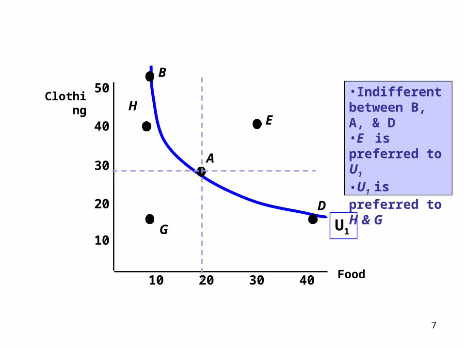
7
Food
10
20
30
40
10 20 30 40
Clothing
50
U1
G
D
A
EH
B•Indifferent between B, A, & D•E is preferred to U1
•U1 is preferred to H & G

8
Indifference Map
Food
Clothing
U2
U3
U1
DB A
Market basket Ais preferred to B.Market basket B ispreferred to D.
9
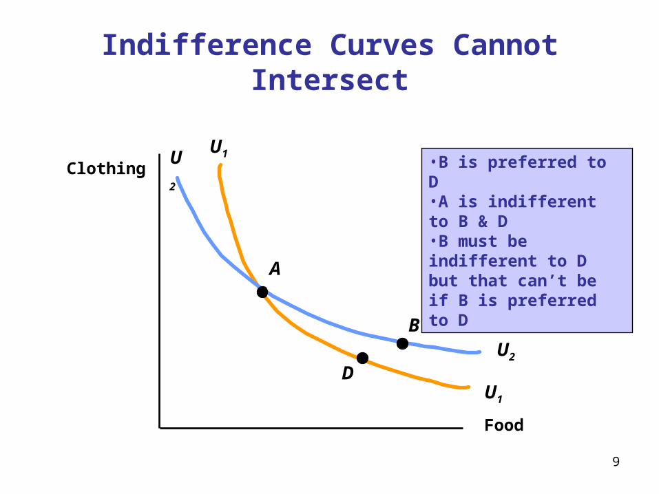
Indifference Curves Cannot Intersect
Food
ClothingU1
U1
U2
U2
D
B
A
•B is preferred to D•A is indifferent to B & D•B must be indifferent to D but that can’t be if B is preferred to D
10
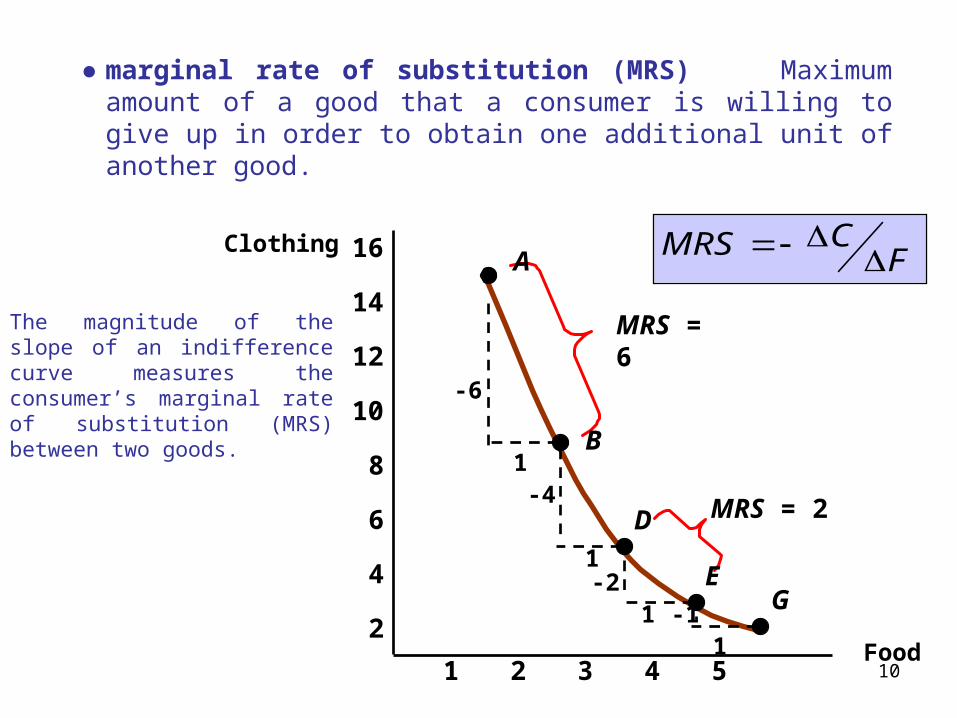
●marginal rate of substitution (MRS) Maximum amount of a good that a consumer is willing to give up in order to obtain one additional unit of another good.
The magnitude of the slope of an indifference curve measures the consumer’s marginal rate of substitution (MRS) between two goods.
Food2 3 4 51
Clothing
2
4
6
8
10
12
14
16 A
B
D
EG
-6
1
1
11
-4
-2-1
MRS = 6
MRS = 2
FCMRS
11
Convexity: The decline in the MRS reflects a diminishing marginal rate of substitution. When the MRS diminishes along an indifference curve, the curve is convex.
As more of one good is consumed, a consumer would prefer to give up fewer units of a second good to get additional units of the first one.
Consumers generally prefer a balanced market basket
12
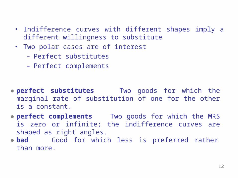
• Indifference curves with different shapes imply a different willingness to substitute
• Two polar cases are of interest– Perfect substitutes– Perfect complements
● perfect substitutes Two goods for which the marginal rate of substitution of one for the other is a constant.
● perfect complements Two goods for which the MRS is zero or infinite; the indifference curves are shaped as right angles.
● bad Good for which less is preferred rather than more.

13
Orange Juice(glasses)
Apple Juice
(glasses)
2 3 41
1
2
3
4
0
PerfectSubstitute
s

14
Right Shoes
LeftShoes
2 3 41
1
2
3
4
0
PerfectComplements
15
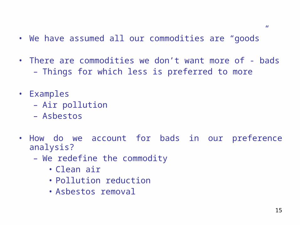
• We have assumed all our commodities are “goods”
• There are commodities we don’t want more of - bads– Things for which less is preferred to more
• Examples– Air pollution– Asbestos
• How do we account for bads in our preference analysis?– We redefine the commodity
• Clean air• Pollution reduction• Asbestos removal
16
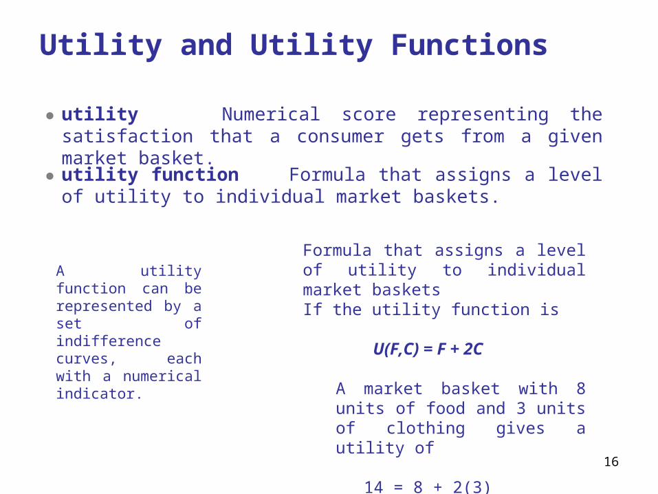
Utility and Utility Functions
● utility Numerical score representing the satisfaction that a consumer gets from a given market basket.
● utility function Formula that assigns a level of utility to individual market baskets.
A utility function can be represented by a set of indifference curves, each with a numerical indicator.
Formula that assigns a level of utility to individual market basketsIf the utility function is
U(F,C) = F + 2C
A market basket with 8 units of food and 3 units of clothing gives a utility of
14 = 8 + 2(3)
17
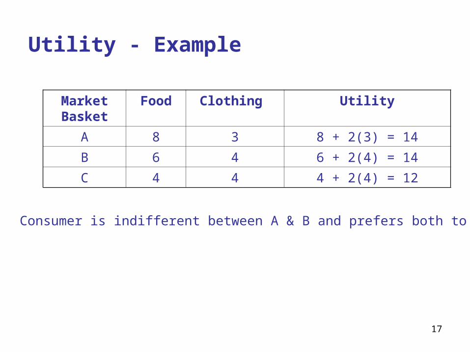
Utility - Example
Market Basket
Food Clothing Utility
A 8 3 8 + 2(3) = 14
B 6 4 6 + 2(4) = 14
C 4 4 4 + 2(4) = 12
Consumer is indifferent between A & B and prefers both to C
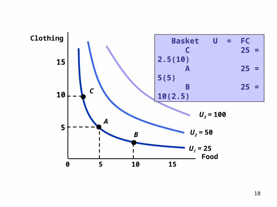
18
Food10 155
5
10
15
0
Clothing
U2 = 50
U1 = 25
U3 = 100A
B
C
Basket U = FC C 25 = 2.5(10) A 25 = 5(5) B 25 = 10(2.5)
19
Ordinal versus Cardinal Utility
●ordinal utility function Utility function that generates a ranking of market baskets in order of most to least preferred.
● cardinal utility function Utility function describing by how much one market basket is preferred to another.
The actual unit of measurement for utility is not important.
An ordinal ranking is sufficient to explain how most individual decisions are made.
20
Budget Constraint
● budget constraints Constraints that consumers face as a result of limited incomes.
● budget line All combinations of goods for which the total amount of money spent is equal to income.
F CP F P C I
21
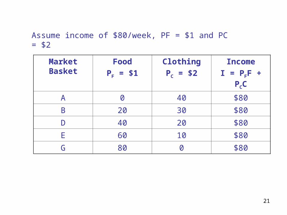
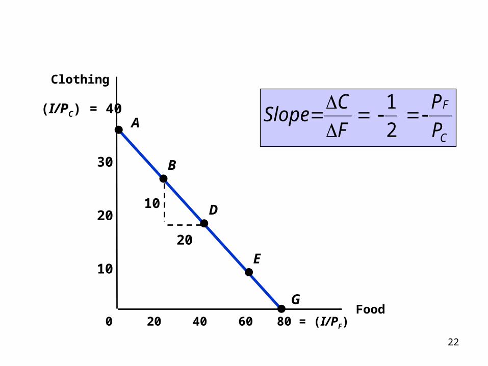
Assume income of $80/week, PF = $1 and PC = $2
Market Basket
FoodPF = $1
ClothingPC = $2
IncomeI = PFF +
PCC
A 0 40 $80
B 20 30 $80
D 40 20 $80
E 60 10 $80
G 80 0 $80
22
(I/PC) = 40
Food40 60 80 = (I/PF)20
10
20
30
0
Clothing
10
20
A
B
D
E
G
C
F
P
P
F
C Slope -
2
1-
23
Budget Line
• As consumption moves along a budget line from the intercept, the consumer spends less on one item and more on the other.
• The slope of the line measures the relative cost of food and clothing
• The slope is the negative of the ratio of the prices of the two goods.
– The vertical intercept (I/PC), illustrates the maximum amount of C that can be purchased with income I.
– The horizontal intercept (I/PF), illustrates the maximum amount of F that can be purchased with income
24
Food(units per week)
Clothing(units
per week)
80 120 16040
20
40
60
80
0
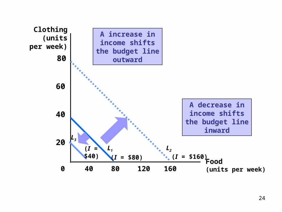
(I = $160)L2
L3
(I =$40) (I = $80)
L1
A increase inincome shifts
the budget lineoutward
A decrease inincome shifts
the budget lineinward

25
The Budget Line - Changes
The Effects of Changes in Prices
– If the price of one good increases, the budget line shifts inward, pivoting from the other good’s intercept.
– If price of food increases and you buy only food (x-intercept), then can’t buy as much food. The point shifts in
– If buy only clothing (y-intercept), can buy the same amount. No change
26
The Budget Line - Changes
– If the price of one good decreases, the budget line shifts outward, pivoting from the other good’s intercept.
– If price of food decreases and you buy only food (x-intercept), then can buy more food. The point shifts out.
– If buy only clothing (y-intercept), can buy the same amount. No change
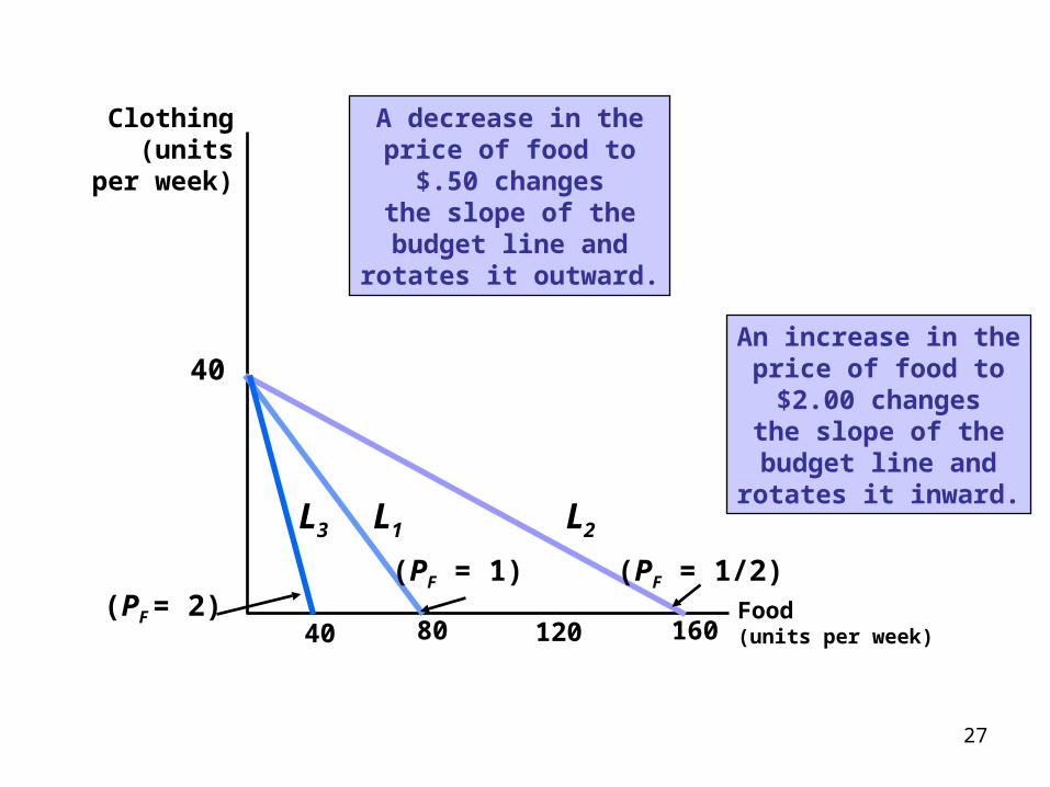
27
40Food(units per week)
Clothing(units
per week)
80 120 160
40
(PF = 1/2)
L2
(PF = 1)
L1L3
(PF = 2)
A decrease in theprice of food to$.50 changes
the slope of thebudget line and
rotates it outward.
An increase in theprice of food to$2.00 changes
the slope of thebudget line and
rotates it inward.
28
The maximizing market basket must satisfy two conditions:
1. It must be located on the budget line.– They spend all their income – more is better
2. It must give the consumer the most preferred combination of goods and services.
• Graphically we can see different indifference curves of a consumer choosing between clothing and food
• Remember that U3 > U2 > U1 for our indifference curves
• Consumer wants to choose highest utility within their budget

29
the slope of an indifference curve is:
F
CMRS
Further, the slope of the budget line is:
C
F
P
PSlope

30
• Optimal consumption point is where marginal benefits equal marginal costs
• MB = MRS = benefit associated with consumption of 1 more unit of food
• MC = cost of additional unit of food– 1 unit food = ½ unit clothing– PF/PC
• If MRS ≠ PF/PC then individuals can reallocate basket to increase utility
• If MRS > PF/PC
– Will increase food and decrease clothing until MRS = PF/PC
• If MRS < PF/PC
– Will increase clothing and decrease food until MRS = PF/PC
31
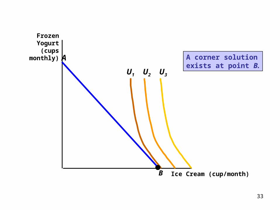
Corner Solution
corner solution Situation in which the marginal rate ofsubstitution of one good for another in a chosen market
basket isnot equal to the slope of the budget line.
When the consumer’s marginal rate of substitution is not equal
to the price ratio for all levels of consumption, a corner solution arises. The consumer maximizes satisfaction by consuming only one of the two goods.
32
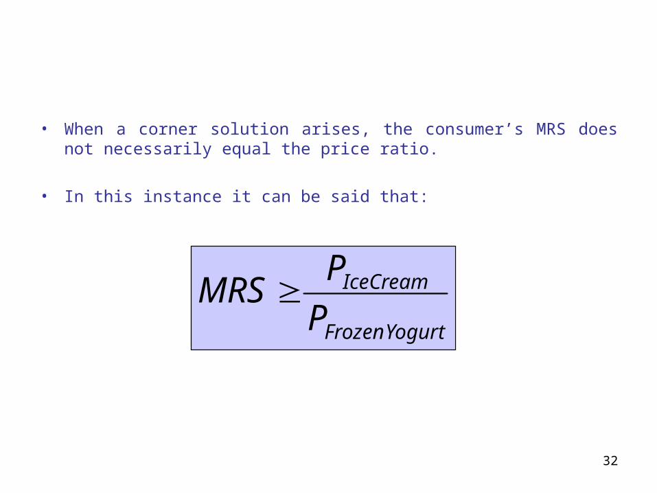
• When a corner solution arises, the consumer’s MRS does not necessarily equal the price ratio.
• In this instance it can be said that:
YogurtFrozen
IceCream
P
PMRS
33
Ice Cream (cup/month)
FrozenYogurt
(cupsmonthly)
U2 U3U1
B
A A corner solutionexists at point B.
34
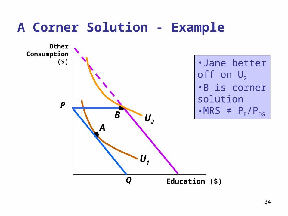
A Corner Solution - Example
Education ($)
OtherConsumption
($)
A
U1
P
Q
B U2
•Jane better off on U2
•B is corner solution•MRS ≠ PE/POG
35
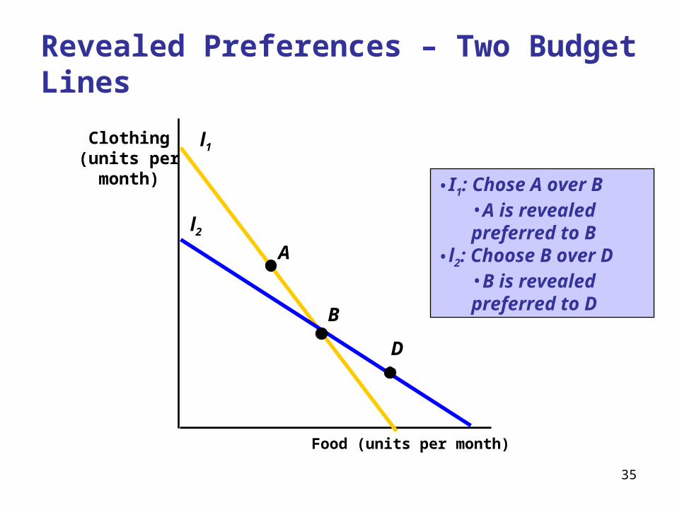
Revealed Preferences – Two Budget Lines
Food (units per month)
Clothing(units per
month)
l1
l2
D
B
A
•I1: Chose A over B•A is revealed preferred to B
•l2: Choose B over D
•B is revealed preferred to D
36
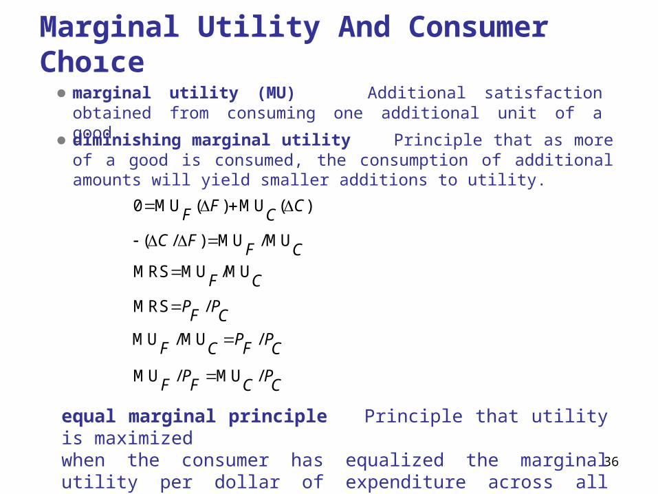
Marginal Utility And Consumer Choıce
0 MU ( ) MU ( )F CF C
● marginal utility (MU) Additional satisfaction obtained from consuming one additional unit of a good.
● diminishing marginal utility Principle that as more of a good is consumed, the consumption of additional amounts will yield smaller additions to utility.
( / ) MU /MUC F F C
MRS MU /MUF C
MRS /P PF C
MU / MU /P PF FC C
MU / MU /P PF F C C
equal marginal principle Principle that utility is maximized when the consumer has equalized the marginal utility per dollar of expenditure across all goods.
37
• Total utility is maximized when the budget is allocated so that the marginal utility per dollar of expenditure is the same for each good.
• This is referred to as the equal marginal principle.

38
Cost-of-Living Indexes
●cost-of-living index Ratio of the present cost of a typical bundle of consumer goods and services compared with the cost during a base period.
● ideal cost-of-living index Cost of attaining a given level of utility at current prices relative to the cost of attaining the same utility at base-year prices.
●Laspeyres price index Amount of money at current year prices that an individual requires to purchase a bundle of goods and services chosen in a base year divided by the cost of purchasing the same bundle at base-year prices.Comparing Ideal Cost-of-Living and Laspeyres Indexes The
Laspeyres index overcompensates Rachel for the higher cost of living, and the Laspeyres cost-of-living index is, therefore, greater than the ideal cost-of-living index.

39
• Chain-Weighted Indexes
– Cost-of-living index that accounts for changes in quantities of goods and services
– Introduced to overcome problems that arose when long-term comparisons were make using fixed weight price indexes
40
● Paasche index Amount of money at current-year prices that an individual requires to purchase a current bundle of goods and services divided by the cost of purchasing the same bundle in a base year.
Comparing the Laspeyres and Paasche Indexes Just as the Laspeyres index will overstate the ideal cost of living, the Paasche will understate it because it assumes that the individual will buy the current-year bundle in the base period.
● fixed-weight index Cost-of-living index in which the quantities of goods and services remain unchanged.