arX

iv:1

211.

5720

v1 [

cs.N

I] 2

5 N

ov 2

012

1

Cognitive Radio Transmission Strategies for

Primary Markovian Channels

Ahmed ElSamadouny, Mohammed Nafie and Ahmed Sultan

Wireless Intelligent Networks Center (WINC)

Nile University, Cairo, Egypt

Email: ahmed.elsamadony@nileu.edu.eg, mnafie@nileuniversity.edu.eg,

salatino@stanfordalumni.org

Abstract

A fundamental problem in cognitive radio systems is that thecognitive radio is ignorant of the

primary channel state and, hence, of the amount of actual harm it inflicts on the primary license holder.

Sensing the primary transmitter does not help in this regard. To tackle this issue, we assume in this paper

that the cognitive user can eavesdrop on the ACK/NACK Automatic Repeat reQuest (ARQ) fed back

from the primary receiver to the primary transmitter. Assuming a primary channel state that follows a

Markov chain, this feedback gives the cognitive radio an indication of the primary link quality. Based

on the ACK/NACK received, we devise optimal transmission strategies for the cognitive radio so as to

maximize a weighted sum of primary and secondary throughput. The actual weight used during network

operation is determined by the degree of protection afforded to the primary link. We begin by formulating

the problem for a channel with a general number of states. We then study a two-state model where

we characterize a scheme that spans the boundary of the primary-secondary rate region. Moreover, we

study a three-state model where we derive the optimal strategy using dynamic programming. We also

extend our two-state model to a two-channel case, where the secondary user can decide to transmit on a

particular channel or not to transmit at all. We provide numerical results for our optimal strategies and

compare them with simple greedy algorithms for a range of primary channel parameters. Finally, we

investigate the case where some of the parameters are unknown and are learned using hidden Markov

models (HMM).

2

I. INTRODUCTION

Cognitive radio technology is a solution to the problem of spectrum under-utilization caused

mainly by static spectrum allocation. In cognitive radio networks, the licensed users coexist with

cognitive users, also known as the secondary or unlicensed users. Primary users are licensed

users who are assigned to certain channels, and they have theright to transmit over the band

of spectrum assigned by regulatory bodies in their respective countries. If other unlicensed, or

secondary, users want to share the spectrum, then they must use the spectrum when it is unused

by the primary users and/or when they can limit the interference they cause on the primary

receivers below a certain specified level. The secondary users attempt to utilize the resources

unused by the primary users adopting procedures that aim at protecting the primary network

from service interruption and interference.

There has been interest in schemes that make use of the feedback of the primary link to predict

the behavior of the primary user in the future and, in the caseof primary channel temporal

correlation, to gain knowledge about the channel between primary transmitter and receiver

(e.g., [1], [2] and [3]). In [1], the secondary user observesthe automatic repeat request (ARQ)

feedback from the primary receiver. The primary user achieved packet rate can be calculated by

counting the ACK feedback messages. The cognitive radio’s objective is to maximize secondary

throughput under the constraint of guaranteeing a certain packet rate for primary user. The

main difference between our work and [1] is that in [1] there is no use of the possible channel

correlation across time, whereas we assume that the primarychannel state follows a Markov

chain. The cognitive transmitter can hence exploit the ACK/NACK feedback messages to predict

the primary channel state during the next transmission phase. In [2], assuming a temporally

correlated channel between the primary transmitter and receiver, the cognitive transmit power is

adjusted based on primary channel state information (CSI) feedback. A real-time fading channel

model is assumed rather than a channel with a finite number of states as we consider and discuss

below. However, the computation of the optimal procedure in[2] is computationally prohibitive.

In [3], the cognitive radio adopts an active sensing protocol where, prior to the sensing, the

cognitive radio generates a temporary jamming signal to deliberately interfere with the primary

user message. If the primary channel is indeed active, the primary network will increase its

transmit power upon receiving the jamming signal. The cognitive radio will receive the power-

3

boosted primary user signal that is more easily detectable.Although this hidden power-feedback

loop should increase the reliability to detect the presenceof the primary user, in our proposed

scheme we assume a passive cognitive radio and the primary link is always active where the

cognitive radio can also transmit during the erasure statesas we will show below.

There has been a series of recent work on cognitive MAC for opportunistic spectrum, e.g., [4],

[5], [8], [9], [10], and [11]. In [4], the primary user activity remains fixed over the duration of a

slot and switches between idle and active states according to a two-state Markovian process. The

channel between the primary transmitter and receiver is notconsidered, and the feedback used to

predict the channel availability is provided by the secondary receiver. However, in our work, the

primary channel is considered and its state changes betweendifferent time slots and the feedback

is provided by the primary receiver not the secondary one. In[5], the work in [4] is extended to

account for energy consumption and spectrum sensing duration optimization. In [8], the authors

focus on the ARQ messages used in primary user data-link-control which are overheard by the

secondary transmitter, which can optimize its access policy by assessing primary user reception

quality. The primary channel is assumed to be of fixed qualityresulting in two fixed and known

packet error rates corresponding to the presence and absence of secondary user transmissions. The

difference between our work and that in [8] is that in our work, the primary channel has different

channel qualities depending on the primary channel state. The more the channel states the primary

channel have, the more the model will be more realistic and the more efficient utilization of

the channel recourses. In [9], the coexistence of two unlicensed links is considered, where one

link interferes with the transmission of the other with quasi-static fading and in the absence

of channel state information at the nodes. The problem is formulated as a Partially Observable

Markov Decision Process (POMDP) and a greedy solution is proposed. In [10], the secondary

source is allowed to superpose its transmissions over thoseof the primary source. The secondary

source aims to maximize its own throughput, while guaranteeing a bounded performance loss for

the primary source. [11] goes along the same line, but considers secondary users cooperation.

In this type of problems the framework of Partially Observable Markov Decision Processes

(POMDP) is usually needed given the uncertainties of the quality of the primary link, and of

the primary user activity as a result of sensing errors [15],[16], [17].

If we assume that the transition probabilities of the underlying Markov chain of the primary

channel is unknown, we use a Hidden Markov Model framework tolearn these transition

4

probabilities. The problem of HMM arises when the actual system state is unknown. HMM is

widely used in many applications. The detailed procedure ofestimating transition probabilities

is provided in [21]. In [23] and [25], HMM has been used for spectrum sensing. The sub-band

occupancy at any time instant can be considered as a state, which can be either free (unoccupied

by a primary user) or busy (occupied by a primary user). The states of a sub-band are monitored

overL consecutive time periods. There are two possible cases discussed in [23]. The first option

is to deal with the situation when the parameters of the HMM and error probabilities are known.

Viterbi algorithm is used to overcome the computational complexity in the likelihood solution.

The second alternative is to deal with the situation when theparameters of Markov chain and the

error probabilities are unknown. Expectation-Maximization (EM) algorithm is used to estimate

these parameters.

Note that HMM has been used in the context of cognitive radioslike in [22] and [24]. In [22],

HMM is used to model and predict the spectrum occupancy of licensed radio bands. In [24],

HMM is used for quickest spectrum detection for cognitive radio where a frequency sweeping

device sweeps the wide-band spectrum and the samples of the wide-band power spectrum density

(PSD) are fed into different HMMs sequentially. In our work,the ARQ is considered as the

secondary user observation vector, which can be consideredas an input to HMM to estimate

the transition probabilities. The quality of estimation depends on the length of the observation

vector.

In this paper, we assume that the primary user is working in a saturation regime where it

always has data to transmit over the primary link. It sends one packet in each time slot, and

receives an ACK or NACK feedback from its receiver at the end of the time slot. The feedback

is received correctly by both the primary and secondary transmitters. The channel between the

primary transmitter and receiver is modeled as a Markov process with a finite number of states

where the channel quality and hence the probability of correct reception is determined by the

state. The state of the channel does not change over a slot. The channel may switch states at

the beginning of each slot according to the transition probabilities of the Markov process. We

laos study the special cases when the primary link follows a two state and a three state Markov

process. The cognitive user exploits the ACK/NACK feedbackfrom the primary receiver to

predict the quality of the primary link. Note that, similar to other papers, this is also a POMDP

problem and we can use techniques similar to other approaches. We assume that one secondary

5

user operates on one primary channel. This is a widely used assumption in the literature. The

system may have a number of orthogonal primary channels where each can be potentially used by

one secondary terminal. At the beginning of each time slot, the secondary user decides whether

to remain silent and listen to primary user feedback, or to carry out transmission. The objective

is to maximize the weighted sum throughput of both the primary and secondary links.

This optimization problem has an exploration-exploitation tradeoff. The tradeoff is between

the choice of the cognitive user activity which maximizes the secondary user throughput, and that

which gives the secondary user knowledge about the channel state information of the primary link

through the ARQ feedback. The correlation between the channel states, via the Markov process,

is what enables us to have this trade-off. A similar trade-off can be achieved if there is correlation

between primary user activity in consecutive time slots [10]. A more general model would be to

assume both correlations. Note that the maximization of theweighted sum throughput can be a

proxy for the optimization problem of maximizing the secondary throughput under a constraint

on the primary throughput [6]. Note however that solving theconstrained optimization problem

is more general.

Our contributions in this paper are as follows. We solve the weighted sum throughput max-

imization problem via modeling it as a dynamic programming problem, and employ Bellman’s

equation [17] to arrive at the optimal strategy. For the two state case, we prove that the optimal

policy is a threshold based policy in the belief of the state of the channel. This threshold can

be obtained numerically. Moreover, when the discounting factor of the dynamic programming

problem approaches unity we obtain a closed form solution tothe weighted sum throughput op-

timization problem, and can find exact description of the strategy that maximizes this throughput

for any weight. Note that changing the weight spans the boundary of the primary-secondary rate

region. We then extend the two state single channel case to the case of a channel with three states

and to the multiple channel case. We obtain numerical solutions to these problems. We then, and

rather than assuming knowledge of the transition probabilities of the above model, investigate

the case where some of the primary network state transition probabilities are unknown, and we

show how to estimate these parameters using Hidden Markov Model (HMM) formulation.

One of the advantages of our scheme is that the ARQ feedback can capture the temporal

correlation in the channel. The cognitive user can access the primary channel in two cases,

when the primary channel quality is relatively high (primary user can transmit successfully

6

regardless of cognitive user activity) and when its qualityis very low (primary user transmission

fails whether secondary user is active or not). This advantage cannot be captured in schemes

employing spectrum sensing only.

The paper is organized as follows. The general multi-state system model and assumptions

are described in Section II. We also introduce in this section the two-state, Gilbert-Elliot, three-

state system models as special cases and the secondary user optimal strategy is obtained using

dynamic programming. In section III, we extend our formulation to the multi-channel case and

specifically address the two channel case. When the secondary user have the chance to choose

a channel from multiple primary channels to transmit on, thesecondary user should choose the

channel that maximizes the reward function as we illustratein Section III. The framework of

Hidden Markov Model (HMM) is used in Section IV to estimate the primary network transition

probabilities if it is unknown given the feedback observations in the form of ARQ feedback.

Numerical results are presented in Section V. Our work is concluded in Section VI.

II. SYSTEM MODEL AND PROPOSEDAPPROACH

Our proposed model assumes that we have one primary link and one secondary link. An

illustration of the setup is provided in Figure 1. We are concerned with the Z-interference

channel model [18] where the interference from the primary transmitter on the secondary receiver

is ignored. The Z-interference channel models important applications such as the interference

caused by macro-cell users on femto-cell receivers, which is known in the literature as the “loud

neighbor” problem. In our context, the primary terminals may be close to one another and use

small transmission power, whereas the cognitive terminalsmay be far from one another and use

high power for communication causing considerable interference on the primary link.

We assume that the primary link is always active, i.e., primary transmitter is working in

saturation regime. The primary link follows a Markov model with S states;1, 2, ..., S. Each

state of theS states describes a certain quality for the primary channel.The secondary user

is aware of the state transition matrix∏

of this Markov chain in addition to the probabilities

of success and failure for primary transmission in each of these states. Table II shows these

probabilities for statei, i = 1, 2, ..., S

Our objective is to choose the transmission strategy that maximizes the expected value of the

7

Sec. silent Sec. transmit

Prob. of success ai bi

Prob. of failure 1− ai 1− bi

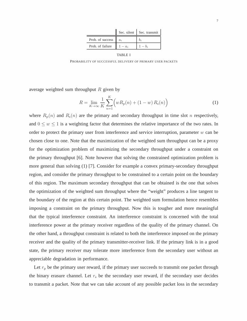
TABLE I

PROBABILITY OF SUCCESSFUL DELIVERY OF PRIMARY USER PACKETS

average weighted sum throughputR given by

R = limK→∞

1

K

K∑

n=1

(

wRp(n) + (1− w)Rs(n))

(1)

whereRp(n) andRs(n) are the primary and secondary throughput in time slotn respectively,

and0 ≤ w ≤ 1 is a weighting factor that determines the relative importance of the two rates. In

order to protect the primary user from interference and service interruption, parameterw can be

chosen close to one. Note that the maximization of the weighted sum throughput can be a proxy

for the optimization problem of maximizing the secondary throughput under a constraint on

the primary throughput [6]. Note however that solving the constrained optimization problem is

more general than solving (1) [7]. Consider for example a convex primary-secondary throughput

region, and consider the primary throughput to be constrained to a certain point on the boundary

of this region. The maximum secondary throughput that can beobtained is the one that solves

the optimization of the weighted sum throughput where the “weight” produces a line tangent to

the boundary of the region at this certain point. The weighted sum formulation hence resembles

imposing a constraint on the primary throughput. Now this istougher and more meaningful

that the typical interference constraint. An interferenceconstraint is concerned with the total

interference power at the primary receiver regardless of the quality of the primary channel. On

the other hand, a throughput constraint is related to both the interference imposed on the primary

receiver and the quality of the primary transmitter-receiver link. If the primary link is in a good

state, the primary receiver may tolerate more interferencefrom the secondary user without an

appreciable degradation in performance.

Let rp be the primary user reward, if the primary user succeeds to transmit one packet through

the binary erasure channel. Letrs be the secondary user reward, if the secondary user decides

to transmit a packet. Note that we can take account of any possible packet loss in the secondary

8

channel when we calculate the value ofrs.

The belief is the secondary user evaluation of the probability of the actual primary link state

in the next time slot given the history of actions and observations. The secondary belief is given

by the vector−→p = (p1p2...pS) with∑S

k=1 pk = 1, wherepk is the probability that the primary

channel is in statek at the beginning of a time slot given all the previous secondary user’s actions

and observations. The belief is updated by the secondary user in each time slot on the basis

of its chosen action during the time slot, the primary ARQ feedback that it observes, and the

primary channel state transition probabilities. Specifically, the secondary user updates this belief

of the primary state according to Markovian update equation−→p n = −→p n−1(updated)

∏

, where−→p n

is the belief vector at time slotn, and−→p n−1(updated) is calculated using the ACK or NACK

overheard from the primary transmitter according to one of the following four cases depending

on the action taken by the secondary user and the corresponding outcome.

Case 1: Secondary user transmits and a NACK is received from the primary network. There-

fore, the secondary belief of the primary channel state during the next time slot is

pi(updated)(1) =P (NACK|i)pi

∑

i P (NACK|i)pi=

(1− ai)pi∑

i(1− ai)pi(2)

wherepi(updated)(l) is the ith element of−→p n−1(updated) for the lth case andP (NACK|i) is the

probability of receiving a NACK given the primary channel state isi.

Case 2: Secondary user transmits and an ACK is received from the primary network. Therefore,

the secondary belief of the primary channel state during thenext time slot is

pi(updated)(2) =P (ACK|i)pi

∑

i P (ACK|i)pi=

aipi∑

i aipi(3)

Case 3: Secondary user is idle and a NACK is received from the primary network. Therefore,

the secondary belief of the primary channel state during thenext time slot is

pi(updated)(3) =(1− bi)pi

∑

i(1− bi)pi(4)

Case 4: Secondary user is idle and an ACK is received from the primary network. Therefore,

the secondary belief of the primary channel state during thenext time slot is

pi(updated)(4) =bipi

∑

i bipi(5)

Then, depending on the case, we have−→p n(l) =−→p n−1(updated)(l)

∏

9

If the secondary user decided to remain silent, the expectedimmediate gain in the next time

slot can be calculated as:

G1(−→p ) = wrpP (ACK|idle) = wrp(

∑

i

aipi) (6)

whereP (ACK|idle) is the probability of receiving an ACK given the secondary user is idle.

If the secondary user is transmitting, the expected immediate gain in the next time slot can be

calculated as:

G2(−→p ) = (1− w)rs + wrpP (ACK|transmit) = (1− w)rs + wrp(

∑

i

bipi) (7)

Thus, the expected immediate reward is:

R(k,−→p , a) =

G1(−→p ) if the secondary user is silent in time slotk

G2(−→p ) if the secondary user is active in time slotk

The optimal strategy is the strategy that maximizes the following discounted reward function

E

K+k−1∑

n=k

αn−k ∗R(n,−→p n, an) | −→p k = p

(8)

V K(−→p ) satisfies the following Bellman equation [17]:

V K(−→p ) = max

wrpP (ACK|idle) + αP (ACK|idle)V K−1(−→p (4))

+ α(1− P (ACK|idle))V K−1(−→p (3)),

(1− w)rs + wrpP (ACK|transmit) + αP (ACK|transmit)V K−1(−→p (2))

+ α(1− P (ACK|transmit))V K−1(−→p (1))

(9)

where

V 1(−→p ) = maxwrpP (ACK|idle), (1− w)rs + wrpP (ACK|transmit) (10)

WhenK = ∞, V (p) denote the maximum achievable discounted reward function.V (p) satisfies

the following Bellman equation [17]:

V (p) = max

wrpP (ACK|idle) + αP (ACK|idle)V (−→p (4)) + α(1− P (ACK|idle))V (−→p (3)),

(1− w)rs + wrpP (ACK|transmit) + αP (ACK|transmit)V (−→p (2))

+ α(1− P (ACK|transmit))V (−→p (1))

(11)

10

The solution can be obtained via Dynamic Programming. We defer the explanation of our

algorithm to the following subsections where we introduce some special cases to better explain

our approach.

A. Erasure/Non-Erasure Channel Model

The primary link follows a two-state Markov chain. This is a special case of the model

described above, whereS=2, and theai’s and bi’s are all ’1’ or ’0’. In particular, we assume

that during each time slot, the primary link is either in an erasure stateE where primary user

transmission always fails or a non-erasure stateN where primary user transmission is successful

when there is no interference. It switches states from one time slot to the next according to a

Markovian process as shown in Figure 2. The process is specified by two parametersPEE and

PNE, wherePEE is the probability that the primary network is in erasure in the next time slot

given that it is in erasure state in the current slot, andPNE is the probability that the primary

network is in erasure in the next time slot given that it is in non-erasure state in the current

slot. We assume that the transition probabilities of the Markov chain are known a priori but we

introduce a technique for estimating them in Section IV. Thetransition matrixP which includes

the transition probabilities is given by

P =

PEE PEN

PNE PNN

Hence, the stationary probabilities of being in erasure andnon-erasure for primary network are

P (E) = PNE

PNE+PENandP (N) = PEN

PNE+PEN, respectively. Note that, the erasure state causes the

primary transmission to fail, while the non-erasure state results in successful packet delivery

to the primary receiveronly when there is no interference from the secondary transmitter. That

is, if the cognitive user decides to transmit in the non-erasure state, its transmission causes the

erasure of the primary user packet.

As long as the cognitive radio is idle, it can eavesdrop on theprimary user ARQ through

which the secondary transmitter can detect the current state of the primary link and, consequently,

decide the erasure probability of the next state whetherPEE or PNE based on the ARQ feedback.

However, if the cognitive radio decides to transmit, it causes the primary user packet to be erased.

The secondary user then overhears a negative acknowledgment (NACK) from the primary receiver

11

no matter what the state of the primary channel is. Thus when the cognitive user transmits, it

becomes unaware of the primary link state because of the collision it causes with the primary

transmitted data. The primary receiver will hence not be able to decode the data, and will send

a negative acknowledgment to its transmitter irrespectiveof its actual channel state. Hence, the

ACK/NACK feedback provides no information because the secondary transmitter is unable to

decide whether the negative ARQ feedback is actually due to the collision or to the fact that the

primary state was in erasure.

The belief here is defined as the probability that primary link is in erasure state at the very

beginning of the time slot from the secondary terminals’s perspective given the history of its

actions and observations. Hence, the expected primary throughput in time slotk as estimated

by the secondary transmitter can be given byrp (1− pk). The belief is updated from one time

slot to another using the Markov property according to the following.

pk =

PEE if current state is erasure

PNE if current state is non-erasure

pk−1PEE + (1− pk−1)PNE if current state is unknown

Note that the third possibility occurs when the secondary user transmits. The expected secondary

throughput in time slotk is as before given byrs

The optimal strategy and maximum throughput can be derived using one of the following

approaches.

1) Dynamic Programming:We propose to use dynamic programming techniques to arrive at

the optimal strategy. The secondary user opportunistically accesses the channel by first synchro-

nizing with the slot structure of primary network. The goal of the secondary user is to transmit

during the erasure states, and allow the primary user to transmit during the non-erasure states

in order to maximize the sum throughput. The main challenge is that the secondary user cannot

know the next state exactly. It has to operate on the basis of its beliefpk. At the beginning of

each time slot, and based on previous actions and observations, the secondary user can calculate

the probabilitypk. Dynamic programming can then be used to find the optimal strategy. The

decision at each value ofpk maximizes the expected reward function and hence the optimal

strategy at time slotk is the strategy that maximizes the following discounted reward function

12

[5]

V K (p) = maxak ,ak+1,...aK+k+1

E

K+k−1∑

n=k

αn−kR (n, pn, an) | pk = p

(12)

where0 ≤ α < 1 is a discounting factor,K ∈ 1, 2, .. is the control horizon, andan is the

action taken at timen. As α decreases, the secondary user puts more emphasis on its short-term

future gains. The termR (n, pn, an) is the reward accrued at instantn when the belief ispn and

the action taken isan. In this paper, the reward is given by

R (n, pn, an) = wRp (n, pn, an) + (1− w)RS (n, pn, an) (13)

whereRp andRs are the primary and secondary throughputs, respectively.

Note that at a certain time instant and a certainpk value, the path through the ”decision tree”

depends on the decision taken-on whether to transmit or not.For that particularpk value at any

other time instant, the optimal decision would not change. Hence we eliminate the subscriptk

because the expected future reward depends only on the valueof p regardless of the index of

the time slot.

If we assume an infinite horizon optimization, and through a dynamic programming argument,

the state of the system can be fully parameterized by the belief that the channel is in erasure

the next time slot,p, where we dropped the time dependence. Hence the action taken by the

cognitive user depends only onp. The belief statep can be updated according to one of the

following three cases depending on the action taken by the secondary user and the corresponding

outcome. We follow here the notation presented in [5].

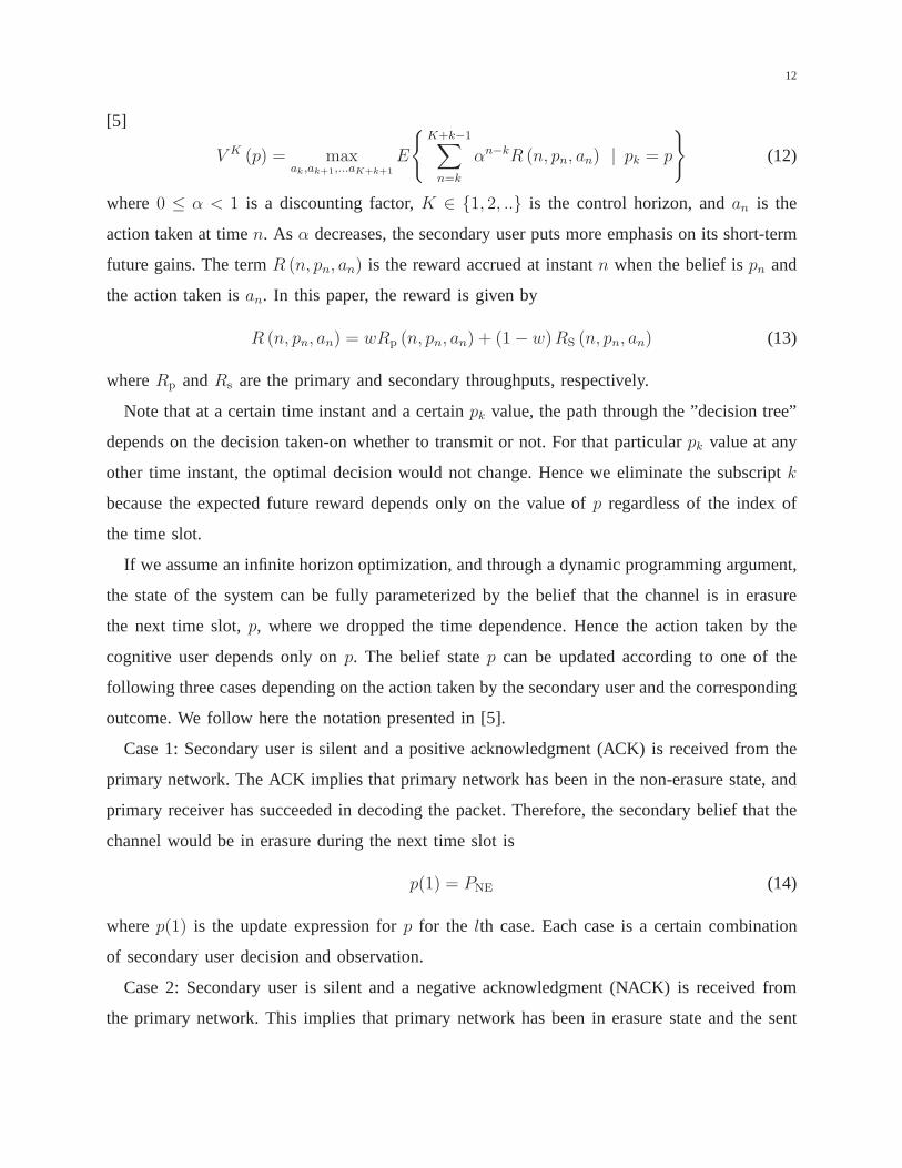
Case 1: Secondary user is silent and a positive acknowledgment (ACK) is received from the

primary network. The ACK implies that primary network has been in the non-erasure state, and

primary receiver has succeeded in decoding the packet. Therefore, the secondary belief that the

channel would be in erasure during the next time slot is

p(1) = PNE (14)

wherep(1) is the update expression forp for the lth case. Each case is a certain combination

of secondary user decision and observation.

Case 2: Secondary user is silent and a negative acknowledgment (NACK) is received from

the primary network. This implies that primary network has been in erasure state and the sent

13

packet has not been delivered successfully. Thus,

p(2) = PEE (15)

Case 3: Secondary user transmits. The probability of erasure is updated by the Markovian

property as follows

p(3) = pPEE + (1− p)PNE (16)

We denote the weighted expected instantaneous throughput when the secondary user listens by

G1 (p) which is given by

G1 (p) = wrp (1− p) (17)

For the case of the secondary user is transmitting, we denotethe weighted expected throughput

by

G2 (p) = (1− w) rs (18)

A greedy scheme would just compareG1(p) with G2(p) and ifG2(p) > G1(p), the secondary

user decides to transmit, otherwise it remains silent. The expected instantaneous reward is:

R(k, p, a) =

G1(p) if the secondary user is silent at time slotk

G2(p) if the secondary user is active at time slotk

Following the definitions in [5], letV K (p) denote the maximum achievable discounted reward

function obtained by maximizing Equation (12). WhenK < ∞, V K (p) satisfies the following

Bellman equation [17]:

V K(p) = max

wrp(1− p) + α(1− p)V K−1 (p(1)) + αpV K−1 (p(2)) ,

(1− w)rs + αV K−1(p(3))

(19)

wherewrp(1 − p) andα(1 − p)V K−1 (p(1)) + αpV K−1 (p(2)) correspond to the expected im-

mediate primary user reward and total discounted future reward respectively if the secondary

user does not transmit, and(1 − w)rs andαV K−1(p(3)) correspond to the expected immediate

secondary reward and total discounted future reward respectively if the secondary user transmits.

V 1(p) = max wrp(1− p), (1− w)rs (20)

14

WhenK = ∞, V K(p) = V K−1(p) = V (p) which satisfies the following Bellman equation:

V (p) = max

wrp(1− p) + α(1− p)V (p(1)) + αpV (p(2)) , (1− w)rs + αV (p(3))

(21)

V (p) can be obtained iteratively. The optimal strategy is obviously a function ofp. We show

in Appendix VII-A that the optimal strategy is a threshold based policy, i.e. the secondary user

will transmit if p > pth. In the next subsection, we present a closed form expressionfor the

maximum throughput and optimal strategy when the discounting factorα tends to unity.

2) Closed Form Solution whenα → 1: We assume thatPEE > PNE making the beliefpk a

monotonic function with time as long as the secondary user istransmitting [19]. This can be

readily seen by solving the first order difference equation governing the evolution ofpk to obtain

pk = (PEE − PNE)Kpk−K +

[

1− (PEE − PNE)K]

P (E) (22)

wherePEE andPNE are Markov chain transition probabilities,P (E) is the steady state probability

of being in an erasure stateE whereP (E) = PNE

PNE+PEN, andpk is the probability of being in

erasure in time slotk.

Using this equation, we can find the probability of erasure intime slot k, pk as a function of

probability of erasure in time slot(k −K), pk−K .

For example, if we consider a single time slot shift(K = 1), we will get the basic Markovian

property.

pk = pk−1PEE + [1− pk−1]PNE

It is clear that ifPEE −PNE > 0, the beliefpk is a monotonic function with time, otherwise the

term (PEE − PNE)K oscillates between positive and negative values.

If the inequality wrp (1− PEE) > (1 − w)rs is satisfied, this implies that the inequality

wrp (1− PNE) > (1− w)rs is also satisfied, sincePEE is greater thanPNE. Thus, from the two

previous inequalities, we can deduce that the optimal secondary user strategy is to listen always

because the expected primary throughput is greater than theexpected secondary throughput re-

gardless of the actual system state, whether it isE or N . Similarly, if wrp (1− PNE) < (1−w)rs,

the optimal secondary strategy is to transmit always. For any other condition, the optimal

secondary strategy is as follows. The secondary transmitter listens as long as an ACK is received

becausewrp (1− PNE) > (1−w)rs and in that case maximizing the throughput in the next time

slot is optimal since we do not affect future decisions as thesecondary user will make use of

15

the knowledge of the next state while it is silent. Once a NACKis received, the secondary user

transmitsM consecutive packets. Thus, the maximization problem in (12) can be reduced to an

optimization problem over the number of secondary user consecutive transmitted packetsM .

It is hence possible to model the system as seen by the secondary user as a 3-state Markovian

chain, where the secondary user either knows that the primary link is in erasure or non-erasure

(while silent) or sendsM-packets without actually knowing the exact state of the primary link.

Figure 3 shows such a representation of our algorithm. The first state N represents the state

that the secondary user is silent and that the primary channel state is in the non-erasure state.

The secondary user overhears an ACK at the end of the primary transmission, and hence the

probability to remain in the same state isPNN and the probability to move to state E isPNE.

The state E refers to the state where the primary link in the erasure state. The secondary user

receives a NACK at the end of the primary user transmission, and hence moves to the “Send

M packets” state. The secondary user transmitsM consecutive packets, then the secondary user

returns back to idle state and starts to listen to the feedback again and returns to state E or N

based on this feedback.

When the Markov chain is in stateN , the primary network achieves a throughput ofrp. When

it is in stateS, the secondary user achieves a throughput ofMrs as the system remains in this

state forM time slots.

In order to find an expression of the throughput as a function of M , we find the stationary

distribution of each state of the Markov chain. Let the steady state probability ofN , E andS

states beP ssN , P ss

E andP ssS respectively, then

P ssN =

1− TM(PEE)

1 + 2PNE − TM(PEE)(23)

P ssE = P ss

S =PNE

1 + 2PNE − TM(PEE)(24)

whereTM(PEE) is the probability of erasure in time slotk given that the state of Markov chain

in time slotk −M was erasure. We can findTM(PEE) from the two-state Markov chain:

TM(PEE) =PNE + (PEE − PNE)

(M+1) (1− PEE)

1 + PNE − PEE(25)

Recall that we assume a positively correlated channel withPEE > PNE.

16

The average primary throughputRp and the average secondary throughputRs can be written

as:

Rp =rpP

ssN

P ssN + P ss

E +MP ssS

(26)

Rs =rsMP ss

S

P ssN + P ss

E +MP ssS

(27)

R(M) = wRp + (1− w)Rs (28)

The problem now becomes to findM that maximize the average weighted sum throughputR(M).

We notice that the optimal value ofM depends on the weightw. The throuhgput obtained using

this scheme spans a number of points on the outer bound of the rate region with the optimal

values ofM (M is integer) that maximize the weighted sum throughput. The outer bound of the

rate region here is piecewise linear, and can be achieved by time division multiplexing between

the different integer values ofM .

Two remarks are in order here:

1. We show in Appendix VII-A that the optimal strategy is a threshold-based policy on the belief

pk, and since the beliefpk is monotonic withM , finding the threshold amounts to finding the

value ofM that maximizes the throughput expression.

2. It can be shown that the throughput is a quasi-concave function of M , and through some

algebraic manipulations, one can arrive at the value ofM that maximizes the throughput. This

can be shown by subtractingR(M) from R(M + 1). TreatingM as a continuous variable, we

can show that this difference has only one positive finite root that is greater than or equal to

unity. By finding this root, we find the value of the unique optimal M . This proof is shown in

the Appendix VII-B.

B. Gilbert-Elliot Model

In the previous model, if the primary channel is in an erasurestate, it will fail to deliver any

packet with probability one, while in a non-erasure state itwill succeed to deliver any packet

with probability one. Here we use the more general model of a good-bad Gilbert-Elliot model (B

andG states), where the probability of successful delivery of a packet depends on the state of the

channel but is not exactly 1 or 0. The probabilities also depend on whether the secondary user

17

is transmitting or not, as discussed before. For example, when the primary channel is in the bad

stateB and the secondary user is silent, there is a probabilityγ1 of receiving an ACK (signifying

correct reception of a packet) from the primary network. Table I gives the probabilities of such

a channel model. This is the same as the general case whenS=2, and here we setγ1 = a1,

γ2 = b1, γ3 = a2 andγ4 = b2.

Sec. silent Sec. transmit

Bad γ1 γ2

Good γ3 γ4

TABLE II

PROBABILITY OF SUCCESSFUL DELIVERY OF PRIMARY USER PACKETS

Typically, the probabilitiesγ1, γ2 andγ4 should be close to zero and the probabilityγ3 should

be close to one. The Erasure/Non-Erasure channel model corresponds to the caseγ1 = γ2 =

γ4 = 0 andγ3 = 1.

The state of the system can be fully parameterized by the belief that the channel is inB state

the next time slot,p. The action taken by the cognitive user depends only onp. The beliefp

can be updated according to one of the following four cases depending on the action taken by

the secondary user and the corresponding outcome.

Case 1: Secondary user transmits and a negative acknowledgment (NACK) is received from

the primary network. Therefore, the secondary belief that the channel would be inB state during

the next time slot is

p(1) = P (B|NACK)PBB + (1− P (B|NACK))PGB (29)

whereP (B|NACK) is the probability ofB state in the current time slot given that the secondary

user receives a NACK in the same time slot andp(k) is the update expression forp for the kth

case.P (B|NACK) can be obtained from Bayes’ rule as follows.

P (B|NACK) =P (NACK|B)P (B)

P (NACK|B)P (B) + P (NACK|G)P (G)

=(1− γ2)p

(1− γ2)p+ (1− γ4)(1− p)(30)

18

Case 2: Secondary user is transmitting and a positive acknowledgment (ACK) is received from

the primary network. Thus,

p(2) = P (B|ACK)PBB + (1− P (B|ACK))PGB (31)

where

P (B|ACK) =P (ACK|B)P (B)

P (ACK|B)P (B) + P (ACK|G)P (G)

=γ2p

γ2p+ γ4(1− p)(32)

Case 3: Secondary user is silent and a NACK is received from the primary network.

p(3) = P (B|NACK)PBB + (1− P (B|NACK))PGB (33)

where

P (B|NACK) =P (NACK|B)P (B)

P (NACK|B)P (B) + P (NACK|G)P (G)

=(1− γ1)p

(1− γ1)p+ (1− γ3)(1− p)(34)

Case 4: Secondary user is idle and an ACK is received from the primary network.

p(4) = P (B|ACK)PBB + (1− P (B|ACK))PGB (35)

where

P (B|ACK) =P (ACK|B)P (B)

P (ACK|B)P (B) + P (ACK|G)P (G)

=γ1p

γ1p+ γ3(1− p)(36)

The parameterp characterizing the belief state is updated by one of the previous four condi-

tions. If secondary user is listening, the expected currentgain can be calculated as:

G1(p) = wrpP (ACK|idle) (37)

whereP (ACK|idle) is the probability of receiving an ACK given the secondary user is idle

P (ACK|idle) = γ1p+ γ3(1− p) (38)

But if the secondary user is transmitting, the expected current gain is:

G2(p) = (1− w)rs + wrpP (ACK|transmit) (39)

19

whereP (ACK|transmit) is the probability of receiving an ACK given the secondary user is

transmitting

P (ACK|transmit) = γ2p+ γ4(1− p) (40)

The expected current reward is:

R(k, p, a) =

G1(p) if the secondary user is silent in time slotk

G2(p) if the secondary user is active in time slotk

The optimal strategy is the strategy that maximizes the following discounted reward function

E

K+k−1∑

n=k

αn−k ∗R(n, pn, an) | pk = p

(41)

V K(p) satisfies the following Bellman equation [17]:

V K(p) = max

wrpP (ACK|idle) + αP (ACK|idle)V K−1(p(4))

+ α(1− P (ACK|idle))V K−1(p(3)),

(1− w)rs + wrpP (ACK|transmit) + αP (ACK|transmit)V K−1(p(2))

+ α(1− P (ACK|transmit))V K−1(p(1))

(42)

where

V 1(p) = maxwrpP (ACK|idle), (1− w)rs + wrpP (ACK|transmit) (43)

WhenK = ∞, V (p) denote the maximum achievable discounted reward function.V (p) satisfies

the following Bellman equation [17]:

V (p) = max

wrpP (ACK|idle) + αP (ACK|idle)V (p(4)) + α(1− P (ACK|idle))V (p(3)),

(1− w)rs + wrpP (ACK|transmit) + αP (ACK|transmit)V (p(2))

+ α(1− P (ACK|transmit))V (p(1))

(44)

We show in Appendix VII-C that the optimum policy is a threshold based policy in the value

of p. We solve Equation (42) numerically. Specifically, we solveit iteratively via approximating

the value function at a finite number of belief values on a grid. The value function is initialized

and then (42) is used to update it. Forp values not belonging to the grid, interpolation or

extrapolation is used. After convergence, the secondary terminal decides whether to transmit or

listen based on the term that maximizesV (p) at each value ofp.

20

C. Three-state System Model

In this subsection, we address the three-state model where the primary channel now follows a

three-state Markov chain whose states are named Bad (B), Good (G) and Very good (Vg) with

transition matrixP where

P =

PBB PBG PBVg

PGB PGG PGVg

PVgB PVgG PVgVg

If the secondary user is listening, the primary user can deliver its packet if the channel state is

G or Vg. But if the secondary user is transmitting, the primary user transmission success is only

in state Vg. This means that the primary and secondary users can both simultaneously transmit

successfully in state Vg. Table III shows the primary packetsuccess or failure during different

channel states and secondary user activities.

Sec. silent Sec. transmit

B fail fail

G success fail

Vg success success

TABLE III

PRIMARY PACKET DELIVERY STATUS DURING DIFFERENT SECONDARY USER ACTIVITY

We can also apply dynamic programming on that system with three channel states to arrive at

the optimal decisions for the secondary user, whether to transmit or to listen, in any situation to

maximize the weighted sum of the primary and secondary throughput.

Here we parameterize the belief state by two parametersp and q, wherep is the probability

that the primary network is in state G in the next time slot andq is the probability that the

primary network is in state Vg in the next time slot. This implies that the probability that the

primary network is in state B is(1− p− q). After each time slot, depending on the action taken

by secondary user and the corresponding feedback,p andq can be updated according to one of

the following four cases.

Case 1: Secondary user is silent and a NACK is received from the primary network. The

NACK during secondary user silence implies that primary network has been in state B and,

21

thus, the primary receiver has failed to receive the packet.Therefore, the belief state in the next

time slot is:

p(1) = PBG (45)

q(1) = PBVg (46)

where, as in the two-state case,p(k) andq(k) are the update expressions forp andq, respectively,

for the kth case.

Case 2: Secondary user is silent and an ACK is received from the primary network. Primary

network could be in state G with probabilitypp+q

or state Vg with probability q

p+q. The belief

state in the next time slot is:

p(2) =p

p+ qPGG +

q

p+ qPVgG (47)

q(2) =p

p + qPGVg +

q

p+ qPVgVg (48)

Case 3: Secondary user is transmitting and an ACK is receivedfrom the primary network.

The ACK during secondary user activity implies that primarynetwork has been in state Vg.

Therefore, the belief state in the next time slot is:

p(3) = PVgG (49)

q(3) = PVgVg (50)

Case 4: Secondary user is transmitting and a NACK is receivedfrom the primary network.

Primary network could be in state G with probabilityp1−q

or state B with probability1−p−q

1−q. The

belief state in the next time slot is:

p(4) =p

1− qPGG +

1− p− q

1− qPBG (51)

q(4) =p

1− qPGVg +

1− p− q

1− qPBVg (52)

Let Qi(p, q), i = 1, 2, 3, 4, denotes the probability that casei above happens:

Q1(p, q) = 1− p− q (53)

22

Q2(p, q) = p+ q (54)

Q3(p, q) = q (55)

Q4(p, q) = 1− q (56)

The parametersp and q characterizing the belief state are updated by one of the previous four

conditions. If secondary user is listening, the expected current gain can be calculated as:

G1(p, q) = wrp(p+ q) (57)

But if the secondary user is transmitting, the expected current gain is:

G2(p, q) = (1− w)rs + wrpq (58)

The expected current reward is:

R(k, p, q, a) =

G1(p, q) if the secondary user is silent in time slotk

G2(p, q) if the secondary user is active in time slotk

The optimal strategy is the strategy that maximizes the following discounted reward function

E

K+k−1∑

n=k

αn−k ∗R(n, pn, qn, an) | pk = p, q0 = q

(59)

V K(p, q) satisfies the following Bellman equation [17]:

V K(p, q) = max

wrp(p+ q) + α∑

i=1,2

Qi(p, q)VK−1(p(i), q(i)),

(1− w)rs + wrpq + α∑

i=3,4

Qi(p, q)VK−1(p(i), q(i))

(60)

where

V 1(p, q) = max wrp(p+ q), (1− w)rs + wrpq (61)

23

When K = ∞, V (p, q) denote the maximum achievable discounted reward function.V (p, q)

satisfies the following Bellman equation [17]:

V (p, q) = max

wrp(p+ q) + α∑

i=1,2

Qi(p, q)V (p(i), q(i)),

(1− w)rs + wrpq + α∑

i=3,4

Qi(p, q)V (p(i), q(i))

(62)

We solve Equation (60) iteratively via approximating the value function at a finite number

of belief values on a two dimensional grid representingp and q values. The value function

is initialized and then (60) is used to update it. Forp and q values not belonging to the grid,

interpolation or extrapolation is used. After convergence, the secondary terminal decides whether

to transmit or listen based on the term that maximizesV (p, q) at each value ofp andq.

III. M ULTIPLE PRIMARY CHANNELS

In this section, we extend the problem of a single primary channel to multiple independent

erasure primary channels with different transition probabilities. The secondary user has to decide

which primary channel to access. Here, we focus on the two channel case. However, this

technique can be extended to the multi-channel case, thoughwith increasing computational

complexity.

We have two independent primary channels with two differenttransition matricesP1 andP2.

P1 =

PEE1 PEN1

PNE1 PNN1

P2 =

PEE2 PEN2

PNE2 PNN2

The system model is exactly similar to the two-state model except that when the cognitive

radio is silent, the secondary transmitter can eavesdrop onthe ARQ from both primary channels

simultaneously. When the secondary user decides to transmit on a specific primary channel, it

can make use of the ARQ from the other primary channel but the ARQ from the occupied

channel carries no information since simultaneous transmission is assumed to surely result in a

NACK.

24

Our objective is to choose the transmission strategy that maximizes the expected value of

weighted sum throughputR given by

R = limK→∞

1

K

K∑

n=1

(

w(Rp1(n, pn, qn, an) +Rp2(n, pn, qn, an)) + (1− w)Rs(n, pn, qn, an))

(63)

whereRp1(n) andRp2(n) are the primary throughput of the first and second channels intime

slot n, respectively,Rs(n) is the secondary throughput in time slotn and 0 ≤ w ≤ 1 is a

weighting factor that determines the relative importance of the two rates,pn, qn are the beliefs

of the two primary channels, andan is the action taken by the secondary user in time slotn.

The cognitive radio action in time slotn, an, is one of the following three different options:

1.Secondary user listens to both primary channels.

2.Secondary user transmits on the first channel and listens to the second channel.

3.Secondary user transmits on the second channel and listens to the first channel.

We can once more apply dynamic programming to this system to find the optimal decisions

for the secondary user. The belief state is parameterized bytwo parametersp andq, wherep is

the probability that the first primary network is in erasure state in the next time slot, andq is

the probability that the second primary network is in erasure state in the next time slot.

After each time slot, depending on the action taken by secondary user and the corresponding

feedback,p can be updated according to one of the following 3 cases:

Case 1: secondary user is not transmitting on the first channel and an ACK is received from

the first primary network. Therefore, the updated value ofp is:

p(1) = PNE1 (64)

Case 2: secondary user is not transmitting on the first channel and a NACK is received from

the first primary network. Therefore, the updated value ofp is:

p(2) = PEE1 (65)

Case 3: secondary user is transmitting on the first channel. The probability of erasure at the

next time slotp is updated by the Markovian property as follows.

p(3) = pPEE1 + (1− p)PNE1 (66)

Similarly, the value ofq is also updated according to one of the previous 3 cases but for the

second primary network:

q(1) = PNE2 (67)

25

q(2) = PEE2 (68)

q(3) = qPEE2 + (1− q)PNE2 (69)

where,p(k) andq(k) are the update expressions forp andq, respectively, for thekth case.

The parametersp and q can be updated by one of the previous conditions according tothe

secondary user decision and the primary networks outputs.

Now, the secondary user has three possible decisions, whether to transmit on the first channel,

to transmit on the second channel or to remain idle and listento both channels feedback.

If secondary user is idle, the expected current gain will be:

G1(p, q) = w(rp1(1− p) + rp2(1− q)) (70)

But if the secondary user transmits on the first channel, the expected current gain is:

G2(p, q) = (1− w)rs + wrp2(1− q) (71)

In case the secondary user transmits on the second channel, the expected current gain is:

G3(p, q) = (1− w)rs + wrp1(1− p) (72)

Therefore, the expected current reward is:

R(k, p, q, a) =

G1(p, q) if the secondary user is idle in time slotk

G2(p, q) if the secondary user is transmitting on first channel in timeslot k

G3(p, q) if the secondary user is transmitting on second channel in time slotk

The optimal strategy is the strategy that maximizes the following discounted reward function

E

K+k−1∑

n=k

αn−k ∗R(n, pn, qn, an) | pk = p

(73)

26

V K(p, q) satisfies the following Bellman equation [17]:

V K(p, q) = max

(w(rp1(1− p) + rp2(1− q)) + α(1− p)(1− q)V K−1(p(1), q(1))+

α(1− p)qV K−1(p(1), q(2)) + αp(1− q)V K−1(p(2), q(1))+

αpqV K−1(p(2), q(2)), (1− w)rs + wrp2(1− q) + αqV K−1(p(3), q(2))+

α(1− q)V K−1(p(3), q(1)), (1− w)rs + wrp1(1− p)+

αpV K−1(p(2), q(3)) + α(1− p)V K−1(p(1), q(3))

(74)

where

V 1(p, q) = maxw(rp1(1− p) + rp2(1− q)),

(1− w)rs + wrp2(1− q), (1− w)rs + wrp1(1− p)(75)

WhenK = ∞, V (p, q) denote the maximum achievable discounted reward function as before.

We solve Equation (74) iteratively via approximating the value function at a finite number

of belief values on a two dimensional grid representingp and q values. The value function

is initialized and then (74) is used to update it. Forp and q values not belonging to the grid,

interpolation or extrapolation is used. After convergence, the secondary terminal decides whether

to transmit on the first channel, transmit on the second channel or listen to both channels based

on the term that maximizesV (p, q) for each value ofp andq.

IV. H IDDEN MARKOV MODEL (HMM)

In previous sections, we assumed that secondary user has full knowledge of the transition

probabilities of the primary network system state. Here, weassume that the cognitive user is not

aware of these transition probabilities. We now divide the time horizon into two intervals, the

first interval is the training period, where the secondary user “learns” the transition probabilities.

The second interval is the transmission interval where the secondary terminal uses the estimated

probabilities in order to derive the optimal transmission policy based on the algorithms presented

in the paper so far. We propose using HMM to estimate the probabilities via listening to the

feedback channel.

The basic idea behind HMM is that the actual system state is unknown. The only available

information is the observation vector, which is a probabilistic function of the state. For example,

27

the three state model can be described as an HMM where the hidden states of the model are B, G

and Vg as mentioned in Section II-C. The ARQ feedback vector (ACK or NACK) is considered

the observation vector. This feedback is generated as mentioned above according to Table III.

Now, we introduce the HMM framework to some of the previouslymentioned models.

A. Two-State System Model

This model is exactly the same as the two-state system model discussed in Section II except

that the transition probabilities are unknown. Hence, the secondary transmitter observes the ARQ

feedback from the primary network and uses this observationvector to estimate the state transition

probabilities of the primary network using an HMM-based scheme. The HMM framework can

be applied to the Erasure/Non-Erasure channel model and theGilbert-Elliot model as well.

Once the transition probabilities are estimated, the same procedure of dynamic programming

presented in Section II is executed to reach the optimal transmission strategy for secondary user

to maximize the weighted sum throughput of the primary and secondary networks.

B. Three-State System Model

HMM framework is also applied to the three-state model, but here, there is a main difference

between the three-state model and the two-state model during applying the HMM framework. In

the two-state model, the secondary user is always silent during transition probabilities estimation

phase because as long as the secondary user is silent, it obtains the maximum knowledge about

the state of the primary channel which will help the secondary user estimate the probabilities

correctly. On the other hand, in the three state model, the transition probabilities estimation

can be refined by both the secondary user silence and transmission. During silence, there is no

uncertainty in the detection of the B state because receiving a NACK feedback, indicates directly

that the previous state is a B state, but if an ACK feedback is received, there is uncertainty

whether the previous state is G or Vg. Also during secondary user transmission, there is no

uncertainty in the detection of state Vg. So a learning scheme would have to combine silence

and transmission during the training phase. For example, the learning procedure using HMM

can start with the secondary user being silent, then these estimation results are considered as an

initial condition for the next phase of learning during which the secondary user is transmitting.

28

V. SIMULATION RESULTS

For all our simulation results, the belief is randomly initialized from a uniform distribution,

then after simulations, it converges to the actual belief. For the two state erasure/non-erasure

channel model, we use the following system parameters:PEE = 0.99, PNE = 0.01, rp = 1 and

rs = 1. The weighted sum of the primary and secondary throughput isshown in Figure 4 which

shows a significant gain in the throughput for our proposed scheme over the greedy scheme

inside the region of interestw > 0.5. Figure 4 also shows that our optimal scheme is very close

to the causal-genie scheme. The causal genie scheme is an upper-bound for the performance

where we assume that a genie informs the secondary user of theprevious primary channel state.

Figure 5 shows the optimal values of the number of secondary user consecutive transmitted

packetsM versus different values of the weighting factorw. We can see from Figure 5 that

in the greedy scheme, the secondary transmitter transmits always (M is infinite) as long as

w < 0.67 which explains the sudden change in the overall throughput at w = 0.67 in Figure

4. The optimal strategy has this threshold atw = 0.5 which means that the secondary user

optimal strategy benefits from learning the channel state rather than transmitting to maximize

its immediate reward. Our proposed scheme spans the boundary of the primary-secondary rate

region at number of points whereM has an integer value. The piecewise linear connection

between these points can be achieved by time division multiplexing between different values of

integerM . For system parametersrp = 1, rs = 1 with the same transition probabilities as above,

the rate region is shown in Figure 6. The rate region is obtained by solving the optimization

problem for various values of the weight,w.

For the three-state model, the system parameters used for generating the simulation results

are as follows:PBB = PGG = PVgVg = 0.9, PBG = PGB = PVgG = 0.005, rp = 1 and rs = 1.

The weighted sum of the primary and secondary throughput is shown in Figure 7. This again

shows that using our scheme of optimization achieves higherthroughput than the greedy scheme

inside the region of interestw > 0.5. This again shows that our scheme of optimization with

maximizing the total future throughput comes between the greedy scheme of maximizing just

the instantaneous reward and the upper-bound of the causal genie.

For the case of two primary channels presented in Section III, we show the throughput that

we obtain using our optimal transmission strategy comparedto the simple greedy model. The

29

two independent primary channels are identical with transition probabilitiesPEE1 = PEE2 =

0.99, PNE1 = PNE2 = 0.01. The secondary user reward isrs = 1 and the primary channels

rewards arerp1 = rp2 = 1. The weighted sum of the primary and secondary throughput isshown

in Figure 8. This figure also shows that our proposed scheme isbetter than greedy scheme for

a region of the weight,w, values.

For the Gilbert-Elliot mode, Table I shows the probability of receiving an ACK from the

primary network in different channel states and secondary user decisions. The numerical pa-

rameters used for the simulation areγ1 = 0.2, γ2 = 0.01, γ3 = 0.95 and γ4 = 0.3. The system

transition probabilities arePEE = 0.8, PNE = 0.1.Figure 9 shows a minor increase of the overall

throughput of our proposed scheme over the greedy scheme.

To evaluate our proposed algorithm of learning the transition probabilities, we simulated the

two-state model as follows. For the Erasure/Non-Erasure channel model, we use a sequence

of observations representing the ARQ feedback for estimating the primary channel transition

probabilities using HMM-based scheme. The actual transition probabilities which need estimation

arePEE = 0.99, PNE = 0.01. The estimation of the transition probabilities versus theobservation

vector length is shown in Figure 10. We can see that estimation is refined by increasing the

length of the observation vector. Figure 11 shows the degradation in the overall throughput

due to using the estimated probabilities using 30 and 100 feedback packets as an observation

vector in the HMM-based scheme instead of the actual probabilities in the optimal strategy

calculations. Figure 11 shows how the length of the observation vector can refine the transition

probabilities estimation and consequently decrease the throughput degradation. Figure 12 shows

the throughput degradation as a function of the observationvector length at a fixed weight w=0.6.

These results show that we can accurately estimate the transition probabilities and suffer limited

loss in throughput if we use around 100 packets in our learning algorithm.

For the Gilbert-Elliot model, the actual transition probabilities we estimate arePEE = 0.8, PNE =

0.1. The estimation of the transition probabilities versus theobservation vector length is shown

in Figure 13. Clearly and expectedly, increasing the lengthof the observation vector leads to

better estimation.

30

VI. CONCLUSION

In this work, the ACK/NACK feedback from the primary receiver is exploited by the secondary

transmitter in order to find optimal transmission strategies that maximize the weighted sum

of primary and secondary throughput. We have formulated theproblem when the number of

primary channel states is ageneral number of statesS. We then tackled the two-state system

model, where we have shown that the optimal transmission strategy is to transmit for a fixed

number of packets,M , after hearing a NACK. We derived an expression forM and derived a

closed-form expression of the optimal overall throughput.For the Gilbert-Elliot model, we have

shown that the optimal strategy is a threshold based policy on the belief of the secondary user

that the primary link is in the erasure state, and used dynamic programming to obtain the optimal

transmission strategy. We have then solved the problem for the case of three channel states and

used dynamic programming to obtain the optimal secondary user policy. For the multiple primary

channels model, we derived the optimal strategy for the secondary user to choose the primary

channel on which to transmit in order to maximize the currentand future reward. In the case

of unknown Markov chain transition probabilities, we proposed using HMM to estimate these

probabilities, and have shown via simulations that close tooptimal performance can be obtained

by using long enough training period.

VII. A PPENDICES

A. Transmission policy of the two-state system is thresholdbased

We show in this appendix that the optimal policy of the two-state system (Erasure/Non-Erasure

channel model) is threshold based in the belief of the secondary user that the primary channel

is in erasure. The reward functionV K(p) is defined as follows.

V K(p) = max

wrp(1− p) + (1− p)V K−1 (p(1)) + pV K−1 (p(2)) ,

(1− w)rs + V K−1(p(3))

(76)

where

V 1(p) = max wrp(1− p), (1− w)rs (77)

If wrp < (1− w)rs, thus, we must havewrp(1− p) < (1− w)rs as0 ≤ p ≤ 1.

This means that

V 1(p) = (1− w)rs (78)

31

V 2(p) = max

wrp(1− p) + (1− p)V 1 (PNE) + pV 1 (PEE) ,

(1− w)rs + V 1(pPEE + (1− p)PNE)

(79)

V 2(p) = max wrp(1− p) + (1− w)rs, (1− w)rs + (1− w)rs (80)

V 2(p) = (1− w)rs (81)

Thus, if wrp < (1− w)rs, we always have

V (p) = (1− w)rs (82)

Hence, secondary user should always transmit.

On the other hand, ifwrp > (1− w)rs

V 1(p) = max wrp(1− p), (1− w)rs (83)

And, since the maximum of two convex and non-increasing functions is also convex and non-

increasing, thus,V 1(p) is convex and non-increasing function inp.

We now use induction to show thatV K(p) is convex and non-increasing for allK.

Lets assume thatV K−1(p) is convex and non-increasing function, we have

V K(p) = max

wrp(1− p) + (1− p)V K−1 (PNE) + pV K−1 (PEE) ,

(1− w)rs + V K−1(p(PEE − PNE) + PNE)

(84)

First term is linear inp, i.e., it is convex. Second term is also convex inp. Hence, by induction,

V K(p) is convex inp. Now, sincePEE > PNE (assumption),V K−1(p) is non-increasing function

in p. Thus,V K−1(PEE) < V K−1(PNE). Thus, first term is non-increasing inp and second term

is also non-increasing inp. Thus, we can deduce,V K(p) is non-increasing function inp. Hence,

V K(p) is convex and non-increasing function inp for all K.

At steady state,

V (p) = max

wrp(1− p) + (1− p)V (PNE) + pV (PEE) ,

(1− w)rs + V (pPEE + (1− p)PNE)

(85)

32

SinceV (p) is convex

V (pPEE + (1− p)PNE) ≤ pV (PEE) + (1− p)V (PNE) (86)

Since(1− w)rs ≤ wrp (otherwise secondary user is always transmitting)

(1− w)rs + V (pPEE + (1− p)PNE) ≤ wrp + pV (PEE) + (1− p)V (PNE) (87)

Therefore, the first and second terms of Equation (85) can be written as

2nd term≤ 1st term+wrpp

Then, if p = 0, 2nd term≤ 1st term, thus, the decision is to listen.

If p = 1

V (p) = maxV (PEE) , (1− w)rs + V (PEE) (88)

V (p) = (1− w)rs + V (PEE). Thus, the decision is to transmit.

Since the first and second terms of Equation (85) are convex and non-increasing functions inp,

the optimal strategy is a threshold based strategy inp, i.e., there is a unique threshold value of

p calledpth at which the secondary user converts from listening to transmitting which represent

the intersection between first term and second term of Equation (85) plotted versusp.

Due to convexity of the first and second terms of Equation (85), the intersectionpth has an upper

and lower bounds as follows.

1−(1− w)rs

wrp< pth < 1−

(1− w)rswrp

PNE (89)

If PEE < pth, the secondary user will listen always whether the channel is in erasure or not, and

if PNE > pth, it will transmit always whether the channel is in erasure ornot.

Thus, for secondary user finite number of transmission, we must haveP (E) < pth < PEE where

P (E) is the stationary probabilities of being in erasure as we also mentioned in Section II

i.e., PNE

PNE+PEN< pth < PEE.

B. Quasi-concavity of the overall rate

Here we will show that the expected throughputR(M) (defined in Equation (28)) has only a

single peak forM ≥ 0. We will show this via showing that the equationR(M +1)−R(M) = 0

33

has only one solution. Using the scheme defined in Section II,the expected overall throughput

R(M) is defined by

R(M) = wRp + (1− w)Rs

=wrpP

ssN

P ssN + P ss

E +MP ssS

+(1− w)rsMP ss

S

P ssN + P ss

E +MP ssS

=wrp(1− TM(PEE)) + (1− w)rsMPNE

1− TM(PEE) + PNE +MPNE(90)

where

TM(PEE) =PNE + (PEE − PNE)

(M+1)(1− PEE)

1 + PNE − PEE(91)

We have

R(M) =wrp(1− PEE − (1− PEE)(PEE − PNE)

(M+1)) + (1− w)rsMPNE(1 + PNE − PEE)

1− PEE − (1− PEE)(PEE − PNE)(M+1) + (M + 1)PNE(1 + PNE − PEE)(92)

Let

A = 1− PEE

B = PEE − PNE

P = PNE

Thus, we have

R(M) =wrp(A− AB(M+1)) + (1− w)rsMP (1− B)

A− AB(M+1) + (M + 1)P (1− B)(93)

Similarly, we have

R(M + 1) =wrpA(1− B(M+2)) + (1− w)rs(M + 1)P (1−B)

A(1−B(M+2)) + (M + 2)P (1− B)(94)

Note that for infiniteM , we haveR(M) ≃ R(M +1). For non-infiniteM , and if there is a peak

at a certain value ofM , we will have a root ofR(M+1)−R(M) = 0. Hence, we want to solve

the difference equationR(M + 1) − R(M) = 0 for M . By substituting in the rate difference

equation and applying some algebraic manipulations, we have

wrpAP (M + 1)(1−B)(1− B(M+2))− wrpAP (M + 2)(1− B)(1− B(M+1))+

(1− w)rs(M + 1)AP (1−B)(1− B(M+1))− (1− w)rsMAP (1 −B)(1− B(M+2))+

(1− w)rsP2(1− B)2 = 0

(95)

34

Let

a = wrpAP (1−B)

b = (1− w)rsAP (1−B)

Thus, we have

((a− b)M + a)(1−B(M+2))− ((a− b)M + a)(1− B(M+1))+

(b− a)(1−B(M+1)) = −(1− w)rsP2(1−B)2

(96)

((a− b)M + a)(1− B)B(M+1) + (a− b)B(M+1) = (a− b)− (1− w)rsP2(1−B)2 (97)

Let

C = (a− b)(1− B)

D = (a− b) + a(1−B)

Now, we have

B(M+1)(CM +D) = (a− b)− (1− w)rsP2(1−B)2 (98)

(M + 1) logB + log(CM +D) = log((a− b)− (1− w)rsP2(1− B)2) (99)

(CM+D) logB+C log(CM+D) = C log((a−b)−(1−w)rsP2(1−B)2)+(D−C) logB (100)

Let

M1 = CM +D

So, we have

M1 logB + C logM1 = C log((a− b)− (1− w)rsP2(1− B)2) + (D − C) logB (101)

C logM1 = K +M1 logB (102)

35

whereK = C log((a− b) − (1 − w)rsP2(1 − B)2) + (D − C) logB is a constant independent

of M1. The solution of the previous equation is the intersection of linear function ofM1 and

logarithmic function ofM1, i.e., the previous equation has at most two solutions.

Note that whenwrp < (1−w)rs, the term((a− b)− (1−w)rsP2(1−B)2) is negative, i.e., the

secondary user should always transmit which is proved in Appendix VII-A.

Otherwise, when(1− w)rs < wrp, we have

logM1 =K −M1 logB

C(103)

Now the roots of the equationR(M + 1)−R(M) are the solutions to the above equation, i.e.,

the intersection between a logarithmic function ofM1 and a linear function ofM1. Note that

both these functions are monotonically increasing(B < 1), and since the slope of a logarithm

is a decreasing function, then if both a logarithmic function and a linear function intersect at

more than one point, then the slope of the logarithmic function has to be higher than the linear

function at the first intersection point. Now we show that themaximum slope of the logarithmic

function is less than the slope of the linear function.

SinceC = (a − b)(1 − B) > 0, then the minimum value ofM1 is D whereM1 = CM +D,

i.e., the minimum is achieved whenM = 0. Thus, the maximum slope of the LHS of Equation

(103) with respect toM1 is 1/D and the slope of RHS is− logBC

.

Now we need to show that1D< − logB

C

CD

=(a− b)(1 −B)

(a− b) + a(1− B)

=(1− b

a)(1−B)

(1− ba) + (1−B)

=(1− (1−w)rs

wrp)(1−B)

(1− (1−w)rswrp

) + (1− B)

=XY

X + Y

WhereX = 1− (1−w)rswrp

andY = 1−B.

By substitution, we have− logB = log( 11−Y

).

Thus, we haveXY

X + Y=

Y

1 + YX

< Y < log(1

1− Y) (104)

36

Which means that1

D< −

logB

C(105)

Equation (105) shows that the maximum slope of the logarithmic term in the LHS of Equation

(103) is always less than the slope of the linear term in the RHS of Equation (103) (recall

that both the linear and logarithmic functions are monotonic functions).Thus, the linear and

logarithmic terms of Equation (103) intersect only once.

Thus, the solution of Equation (102) with respect toM1 has a unique solution which leads to

the optimal number of secondary user consecutive transmissionsM .

C. Transmission policy of Gilbert-Elliot model is a threshold based policy

As we mentioned in Section II-B, imperfect ACK/NACK reception is assumed. Table I shows

the probability of receiving an ACK from the primary networkin different channel states and

secondary user decisions. The reward functionV K(p) is defined as follows.

V K(p) = max

wrpP (ACK|idle) + P (ACK|idle)V K−1(p(4))+

(1− P (ACK|idle))V K−1(p(3)), (1− w)rs + wrpP (ACK|transmit)+

P (ACK|transmit)V K−1(p(2)) + (1− P (ACK|transmit))V K−1(p(1))

(106)

where

p(1) = P (E|NACK, transmit)PEE + (1− P (E|NACK, transmit))PNE

=(1− γ2)p

(1− γ2)p+ (1− γ4)(1− p)

[

PEE − PNE

]

+ PNE

p(2) = P (E|ACK, transmit)PEE + (1− P (E|ACK, transmit))PNE

=γ2p

γ2p+ γ4(1− p)

[

PEE − PNE

]

+ PNE

p(3) = P (E|NACK, idle)PEE + (1− P (E|NACK, idle))PNE

=(1− γ1)p

(1− γ1)p+ (1− γ3)(1− p)

[

PEE − PNE

]

+ PNE

p(4) = P (E|ACK, idle)PEE + (1− P (E|ACK, idle))PNE

=γ1p

γ1p+ γ3(1− p)

[

PEE − PNE

]

+ PNE

37

and

V 1(p) = max wrp(pγ1 + (1− p)γ3) , (1− w)rs + wrp(pγ2 + (1− p)γ4)

= max wrpp(γ1 − γ3) + wrpγ3 , (1− w)rs + wrpp(γ2 − γ4) + wrpγ4

Let γ3 > γ1 andγ4 > γ2 which is an intuitive assumption which indicates that the probability of

receiving an ACK in the Non-erasure state is greater than that in the Erasure state. Thus,V 1(p)

is convex and non-increasing function inp.

Similar to the Erasure/Non-Erasure channel model, we use induction to show thatV K(p) is

convex and non-increasing in its argument and let’s assume that V K−1(p) is convex and non-

increasing function, we have

V K(p) = max

wrp(pγ1 + (1− p)γ3) + (pγ1 + (1− p)γ3)VK−1(p(4))+

(1− pγ1 − (1− p)γ3)VK−1(p(3)), (1− w)rs + wrp(pγ2 + (1− p)γ4)+

(pγ2 + (1− p)γ4)VK−1(p(2)) + (1− pγ2 − (1− p)γ4)V

K−1(p(1))

(107)

dp(1)dp

=

[

(1− γ2)p+ (1− γ4)(1− p)]

(1− γ2)− (1− γ2)p[

(1− γ2)− (1− γ4)]

[

(1− γ2)p+ (1− γ4)(1− p)]2

[

PEE − PNE

]

=(1− γ2)(1− γ4)

[

(1− γ2)p+ (1− γ4)(1− p)]2

[

PEE − PNE

]

dp(2)dp

=

[

γ2p+ γ4(1− p)]

γ2 − γ2p[

γ2 − γ4]

[

γ2p+ γ4(1− p)]2

[

PEE − PNE

]

=γ2γ4

[

γ2p+ γ4(1− p)]2

[

PEE − PNE

]

Similarly,

dp(3)dp

=(1− γ1)(1− γ3)

[

(1− γ1)p+ (1− γ3)(1− p)]2

[

PEE − PNE

]

dp(4)dp

=γ1γ3

[

γ1p+ γ3(1− p)]2

[

PEE − PNE

]

SincePEE > PNE, we can see thatdp(1)dp

, dp(2)dp

, dp(3)dp

, and dp(4)dp

are greater than or equal to zero.

This means thatp(1), p(2), p(3), andp(4) are non-decreasing inp.

38

Lets start with the monotonicity proof ofV K(p) in Equation (107).

The termswrp(pγ1 + (1− p)γ3) = wrp(γ3 − p[γ3 − γ1]) and (1− w)rs + wrp(pγ2 + (1− p)γ4)

are non-increasing inp asγ3 > γ1 andγ4 > γ2.

Assuming thatV K−1(p) is non-increasing in its argument, we study now the monotonicity of

Ω1(p) where

Ω1(p) = (pγ1 + (1− p)γ3)VK−1(p(4)) + (1− pγ1 − (1− p)γ3)V

K−1(p(3))

dΩ1(p)

dp=− (γ3 − γ1)V

K−1(p(4)) + (pγ1 + (1− p)γ3)dV K−1(p(4))

dp(4)

dp(4)

dp

+ (γ3 − γ1)VK−1(p(3)) + (1− pγ1 − (1− p)γ3)

dV K−1(p(3))

dp(3)

dp(3)

dp

dΩ1(p)

dp=(pγ1 + (1− p)γ3)

dV K−1(p(4))

dp(4)

dp(4)

dp+ (1− pγ1 − (1− p)γ3)

dV K−1(p(3))

dp(3)

dp(3)

dp

− (γ3 − γ1)[VK−1(p(4))− V K−1(p(3))]

(108)

Note that

p(3)− p(4) =[ 1− γ1(1− γ1)p+ (1− γ3)(1− p)

−γ1

γ1p+ γ3(1− p)

]

p[

PEE − PNE

]

=(γ3 − γ1)(1− p)p

[γ1p+ γ3(1− p)][(1− γ1)p+ (1− γ3)(1− p)]

[

PEE − PNE

]

≥ 0

i.e., p(3) ≥ p(4) and sinceV K−1(p) is non-increasing in its argument. Thus,V K−1(p(4)) ≥

V K−1(p(3)).

In Equation (108), sincedp(3)dp

and dp(4)dp

are≥ 0, and dV K−1(p(3))dp(3)

and dV K−1(p(4))dp(4)

are≤ 0. Thus,dΩ1(p)

dp≤ 0, i.e.,Ω1(p) is non-increasing inp.

The same can be shown forΩ2(p) where

Ω2(p) = (pγ2 + (1− p)γ4)VK−1(p(2)) + (1− pγ2 − (1− p)γ4)V

K−1(p(1))

by just replacingγ1, γ3, p(3), andp(4) by γ2, γ4, p(1), andp(2) respectively.

SinceV 1(p) is a monotonically non-increasing inp, by inductionV K(p) is non-increasing inp.

Now, we will proof the convexity ofV K(p).

39

The linear termswrp(pγ1+(1−p)γ3) and(1−w)rs+wrp(pγ2+(1−p)γ4) are convex. Assuming

V K−1(p) is convex inp,

d2Ω1(p)

dp2=2(γ3 − γ1)

dV K−1(p(3))

dp(3)

dp(3)

dp− 2(γ3 − γ1)

dV K−1(p(4))

dp(4)

dp(4)

dp

+ (pγ1 + (1− p)γ3)[d2V K−1(p(4))

dp2(4)

(dp(4)

dp

)2

+dV K−1(p(4))

dp(4)

d2p(4)

dp2

]

+ (1− pγ1 − (1− p)γ3)[d2V K−1(p(3))

dp2(3)

(dp(3)

dp

)2

+dV K−1(p(3))

dp(3)

d2p(3)

dp2

]

(109)

where

d2p(3)dp2

= −2(1− γ1)(1− γ3)(γ3 − γ1)

[

(1− γ1)p+ (1− γ3)(1− p)]3

[

PEE − PNE

]

d2p(4)dp2

=2γ1γ3(γ3 − γ1)

[

γ1p+ γ3(1− p)]3

[

PEE − PNE

]

d2Ω1(p)

dp2=(pγ1 + (1− p)γ3)

d2V K−1(p(4))

dp2(4)

(dp(4)

dp

)2

+

(1− pγ1 − (1− p)γ3)d2V K−1(p(3))

dp2(3)

(dp(3)

dp

)2(110)

since d2V K−1(p(3))dp2(3)

and d2V K−1(p(4))dp2(4)

are≥ 0.

Therefore,d2Ω1(p)dp2

≥ 0. The same procedure can be applied to prove thatd2Ω2(p)dp2

≥ 0.

By induction,V K(p) is convex.

The two terms ofV K(p) in Equation (107) are convex and non-increasing. Thus, the optimal

strategy is a threshold based policy inp and there is a unique optimal solution.

REFERENCES

[1] K. Eswaran, M. Gastpar, and K. Ramchandran, “Bits through ARQs: Spectrum Sharing with a Primary Packet System”,

IEEE Int. Symp. Inf. Theory (ISIT) Nice, France, June 2007.

[2] D. Hamza and M. Nafie, “Throughput Maximization Over Temporally Correlated Fading Channels in Cognitive Radio

Networks”, IEEE Int. Conf. on Telecomm. (ICT) Doha, Qatar, April 2010.

[3] R. Zhang and Y. C. Liang, “Exploiting Hidden Power-Feedback Loops for Cognitive Radio”,in DySPAN 2008. 3rd IEEE

Symp.. 54(5), pp.922-933., oct. 2008.

[4] Q. Zhao, L. Tong, A. Swami, and Y. Chen, “Decentralized Cognitive MAC for Opportunistic Spectrum Access in Ad Hoc

Networks: A POMDP Framework”,IEEE Journal on Selected Areas in Communications, vol. 25, no. 3, pp. 589600, April,

2007.

40

[5] A. T. Hoang, Y. C. Liang, D. T. C. Wong, Y. Zeng, and R. Zhang, “Opportunistic Spectrum Access for Energy-Constrained

Cognitive Radios”,IEEE Vehicular Technology Conf. (VTC) Singapore, May 2008.

[6] R. Cendrillon, W. Yu, M. Moonen, J. Verlinden, and T. Bostoen, “Optimal Multiuser Spectrum Balancing for Digital

Subscriber Lines”,IEEE Trans. Commun., pp.1-5, May 2006.

[7] S. Boyd, L. Vandenberghe, “Convex Optimization”, 1st ed. Cambridge University Press, 2006, pp.178-179.

[8] F. E. Lapiccirella, Z. Ding, and X. Liu, “Cognitive Spectrum Access Control Based on Intrinsic Primary ARQ information”,

IEEE International Conference on Communications, ICC2010, Cape Town, South Africa, May, 2010.

[9] M. Levorato, O. Simeone, and U. Mitra, “Interference Management via Rate Splitting and HARQ over Time-Varying Fading

Channels”,Proc. of ACM Coronet (ACM Mobicom symposium), 2009, Beijing, Cina, 2009.

[10] M. Levorato, U. Mitra, and M. Zorzi, “Cognitive Interference Management in Retransmission-Based Wireless Networks”,

47th Allerton Conference on Communication, Control, and Computing, Sept. 2009.

[11] M. Levorato, O. Simeone, U. Mitra, and M. Zorzi, “Cooperation and Coordination in Cognitive Networks with Packet

Retransmission”,Information Theory Workshop (ITW), 2009.

[12] L. Badia, M. Levorato, and M. Zorz, “Markov analysis of selective repeat type II hybrid ARQ using block codes”,IEEE

Trans. Commun., vol. 56, no. 9, pp. 14341441, Sep. 2008

[13] F. Shi, D. Yuan, and L. X, “Performance analysis of Type-III HARQ scheme in cross-layer design for QoS-guaranteed

traffic”, IEEE Proc. of the Int. Workshop on Cross Layer Desig, pp. 133-137, Sept. 2007

[14] S. Tomasin, M. Levorato, and M. Zorzi, “Analysis of outage probability for cooperative networks with HARQ”,Proc.

IEEE ISIT 2007,, Nice, France, June 2007

[15] A. K. Karmokar, D. V. Djonin, and V. K. Bhargav, “POMDP-based coding rate adaptation for type-I hybrid ARQ systems

over fading channels with memory”,IEEE Trans. Wireless Commun., vol. 5, no. 12, pp. 3512-3523, Dec. 2006.

[16] S. Russel and P. Norvig, “Artificial Intelligence: A Modern Approach, Second Edition.”, Prentice Hall, 2003.

[17] D. P. Bertsekas,“Dynamic Programming and Optimal Control”, 2nd ed., vols. 1 and 2. Athena Scientific,2001.

[18] S. Vishwanath, N. Jindal, and A. Goldsmith, “The Z channel”, Global Communication Conference, December 2003.

[19] K. Liu and Q. Zhao, “Indexability of Restless Bandit Problems and Optimality of Whittle’s Index for Dynamic Multichannel

Access”,IEEE Transactions on Information Theory, November, 2008.

[20] W. Lovejoy, “Computationally feasible bounds for partially observed Markov decision processes”,Operations Research,

39(1):162175, 1991.

[21] R. R. Lawrence., “A tutorial on hidden markov models andselected applications in speech recognition”,Proceeding of

the IEEE, Vol. 77(2), pp. 257-286, 1989.

[22] I. A. Akba and W. H. Tranter, “Dynamic spectrum allocation in cognitive radio using hidden markov models: Poisson

distributed case”,IEEE Southeast Conference, pp. 196-201, 2007.

[23] C. Ghosh, “Innovative Approaches to Spectrum Selection, Sensing, and Sharing in Cognitive Radio Networks”, PhD Thesis,

University of Cincinnati, May 2009.

[24] Z. Chen, Z. Hu, and R. Qiu, “Quickest Spectrum DetectionUsing Hidden Markov Model for Cognitive Radio”,IEEE

Military Communications, 2009.

[25] C. Ghosh, C. Cordeiro, D. P. Agrawal, and M. B. Rao, “Markov Chain Existence and Hidden Markov Models in Spectrum

Sensing”,IEEE PerCom 2009, Mar. 2009.

FIGURES

41

Fig. 1. Z-interference erasure channel model. The secondary transmitter, when active, causes interference on the primary

receiver. The secondary receiver, on the other hand, is shadowed from the primary transmitter, thereby suffering no interference

from it. ENC is the channel encoder, whereas DEC is the receive decoder.

Fig. 2. Two-state Markov model.

Fig. 3. Closed Form Solution whenα → 1.

42

0 0.1 0.2 0.3 0.4 0.5 0.6 0.7 0.8 0.9 1

0.4

0.5

0.6

0.7

0.8

0.9

1

weight (w)

over

all t

hrou

ghpu

t=w

*Rp+(

1−w

)*R

s

Optimal strategyGreedy schemeCausal−genie scheme

Fig. 4. Two-state weighted sum throughput.

0.4 0.5 0.6 0.7 0.8 0.9 10

20

40

60

80

100

120

140

160

180

200

weight (w)

Num

ber

of s

econ

dary

con

secu

tive

tran

smitt

ed p

acke

ts (

N)

Optimal strategyGreedy scheme

Fig. 5. Optimal number of consecutive transmitted packets.

0 0.05 0.1 0.15 0.2 0.25 0.3 0.35 0.4 0.45 0.50

0.1

0.2

0.3

0.4

0.5

0.6

0.7

0.8

0.9

1

primary throughput

seco

ndar

y th

roug

hput

Fig. 6. primary-secondary rate region.

43

0 0.1 0.2 0.3 0.4 0.5 0.6 0.7 0.8 0.9 10.55

0.6

0.65

0.7

0.75

0.8

0.85

0.9

0.95

1

weight (w)

over

al th

roug

hput

=W*R

p+(

1−w

)*R

s

Optimal strategyGreedy schemeCausal−genie scheme

Fig. 7. Three-state weighted sum throughput.

0 0.1 0.2 0.3 0.4 0.5 0.6 0.7 0.8 0.9 10.75

0.8

0.85

0.9

0.95

1

weight (w)

over

al th

roug

hput

=w*(

Rp1

+Rp2

)+(1

−w)*

Rs

Optimal strategyGreedy schemeCausal−genie scheme

Fig. 8. Two-channel two-state weighted sum throughput.

0 0.1 0.2 0.3 0.4 0.5 0.6 0.7 0.8 0.9 10.4

0.5

0.6

0.7

0.8

0.9

1

weight (w)

over

all t

hrou

ghpu

t=w

*Rp+(

1−w

)*R

s

Optimal strategyGreedy schemeCausal−genie scheme

Fig. 9. Weighted sum throughput for the Gilbert-Elliot Model.

44

20 40 60 80 100 120 140 160 1800

0.1

0.2

0.3

0.4

0.5

0.6

0.7

0.8

observation vector length

Tra

nsiti

on p

roba

bilit

ies

PEE

PNE

Fig. 10. Transition probabilities estimation.

0 0.1 0.2 0.3 0.4 0.5 0.6 0.7 0.8 0.9 10.2

0.3

0.4

0.5

0.6

0.7

0.8

0.9

1

weight (w)

over

all t

hrou

ghpu

t

Optimal throughput using actual probabilitiesThroughput using estimated probabilities with 30 packets observation vectorThroughput using estimated probabilities with 100 packets observation vector

Fig. 11. Throughput degradation due to estimation error.

100 200 300 400 500 600 700 800 900 10000.4

0.41

0.42

0.43

0.44

0.45

0.46

0.47

0.48

0.49

observation vector length

over

all t

hrou

ghpu

t

Optimal throughput using actual probabilities(w=0.6)Throughput using estimated probabilities(w=0.6)

Fig. 12. Throughput degradation due to estimation error at weight w = 0.6.

45

20 40 60 80 100 120 140 160 1800

0.1

0.2

0.3

0.4

0.5

0.6

0.7

0.8

observation vector length

Tra

nsiti

on p

roba

bilit

ies

PEE

PNE

Fig. 13. Transition probabilities estimation for the Gilbert-Elliot Model.