1

Clock Distribution

Rajeev Murgai

Advanced CAD Technologies

Fujitsu Labs of America

UC Berkeley

Feb 15, 2005

2

Defining Clock Skew and Jitter

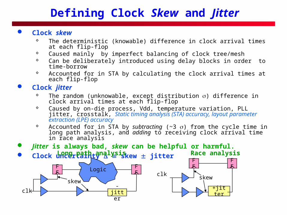
Clock skew The deterministic (knowable) difference in clock arrival times at each flip-flop Caused mainly by imperfect balancing of clock tree/mesh Can be deliberately introduced using delay blocks in order to time-borrow Accounted for in STA by calculating the clock arrival times at each flip-flop

Clock jitter The random (unknowable, except distribution ) difference in clock arrival

times at each flip-flop Caused by on-die process, Vdd, temperature variation, PLL jitter, crosstalk,

Static timing analysis (STA) accuracy, layout parameter extraction (LPE) accuracy

Accounted for in STA by subtracting (~3 ) from the cycle time in long path analysis, and adding to receiving clock arrival time in race analysis

Jitter is always bad, skew can be helpful or harmful. Clock uncertainty skew jitter

Logic

-jitter

FF

FF

clk

FF

FF

+jitter

clk

Long path analysis Race analysis

skewskew

3

Background

Technology scaling results in: higher clock frequencies possible and requested by users prominence of wiring parasitics (R,L,C) in electrical behavior increasing noise impact on delays increasing on-chip process variation impact on delays

Existing ASIC clock synthesis flows Use tree architectures: not best for low skew, jitter, variations Don't properly address noise issues Rely on STA to calculate the delays through clock networks Use inaccurate wiring models Use noise-sensitive clock circuit topologies Ignore or crudely estimate process/voltage/temperature variations Don’t have tight integration of physical synthesis & clock synthesis

Result Predictability of clock delay is poor: Clock uncertainty (i.e., skew +

jitter) of 400ps is not uncommon Maximum attainable clock frequency is impaired

4

Problems with Existing Clock Methodologies

Tree-based Clock Distribution Low power but... Sensitive to mismatching branches, difficult to layout Sensitive to noise, especially if wires are not shielded Using STA to calculate tree timing results in large errors => high skew and jitter

PLL

FF

FF

FF

FF

large skew and jitter

FF

FF

medium skew and jittersmall skew and jitter

5

Problems with Static Timing Analysis (STA)

LR

CgCs

What we have...

signal wire

What STA uses...

CloadCw/2Cw/2

Rwire

Rup

Rdn

Note: driver model is a little better than this with table look-up

Other problemsCw can match either delay or slew, but not bothinterpolation using look-up tables

6

Clock Distribution Architectures

Two basic architectures Tree Grid (mesh)

Hybrids of tree and mesh Tree + crosslinks Mesh + local trees

7

Tree

Widely used in ASICs

Advantages Low cost

– Wiring– Capacitance– Power

Clock gating easy

Disadvantages Difficult to balance path

delays due to asymmetric FF distribution

Sensitive to variations Topologies

Symmetric H-tree Asymmetric trees

Flip-flops

8

CAD for Tree Architecture

Topology generation H-tree: widely used Method of means and medians (MMM) [Jackson et al. DAC 90]

– Goal: reduce wirelength while minimizing skew.– Divide set S of points into Sleft and Sright, based on median.

| Sleft | = | Sright |– Connect/route center of mass (CM) of S to CM of Sleft and Sright.– Recurse on Sleft and Sright.

9

Method of Means & Medians

Problem May not result in zero skew

Solution One step look-ahead and decide direction of splitting.

– Estimate skews using Penfield Rubenstein model.

Other problems Buffer insertion not handled. Obstructions not handled.

10

Topology: Recursive Geometric Matching

[Kahng et al. DAC 91]

Bottom-up pair-wise merge algorithm

Optimum geometric matching on n points (minimum wirelength)

Determine center point of each match edge

Recurse on n/2 points

Uses path length skews

Tries to balance root to leaf path lengths.

11

Topology: Simulated Annealing

Topology generation

Cheng et al: improve initial topology by simulated annealing

– effective in reducing delay

12

CAD for Tree Architecture

Routing & wire sizing Tsay, TCAD 93: zero-skew routing

– first paper to use Elmore delay as delay model earlier work used pathlength

DME, planar DME– make faster paths slower by detours/snaking to match delays– may use wire-sizing: make slower paths faster

Wire spacing

Buffering Tellez & Sarrafzadeh, TCAD 97 insert minimum buffers on a given topology to meet skew and slew

constraints.

13

Grid/Mesh

n x n uniform mesh

Distributed array of k x k buffers drives the mesh.

Buffers driven by global H-tree.

Flip-flops directly connected to the nearest mesh segment

Used in modern processors

Advantages Excellent for low skew Robust to variations

Disadvantages Higher wiring area,

capacitance, power Difficult to analyze

– Loops and redundancy

flip flops

Clock source

14

Mesh

Sizing of clock distribution networks for high performance CPU chips Desai et al., DEC [DAC 1996] goal: size grid interconnect segments with constraints on clock latency

and average current assume: initial grid and interconnect sizes width explicit => non-linear program; practical for small networks/trees. consider width as implicit & solve using sequence of network problems. Results: applied on clock networks of two actual processors: DC21046A

and DC21164. Results for DC21046A: – 275MHz clock– grid has 1 million edges, 15.5K drivers, 81K receivers– 16% reduction in capacitance - without increasing clock latency.– Runtime: 3 days.

Optimal Wire and Transistor Sizing for Circuits with Non-tree Topology Vandeberghe et al., Stanford University [ICCAD 97] RC circuit with tree topology => sizing problem is convex optimization meshes have R loops; use dominant time constant as measure of delay solve using semi-definite programming (quasi-convex function)

15

Hybrid Architecture: Tree + Cross-links

Reducing Clock Skew Variability via Cross Links [Rajaram et. al., DAC 2004]

tree + short-circuit some sink pairs => non-tree topology clock signal propagates through multiple paths; reduces skew and

skew variability between shorted sinks

reduces skew variability by 30-70%

very small wire-length penalty (2%) over tree topology

Drawback: does not consider buffering source

16

Hybrid Architecture: Mesh + Trees

source

Hybrid Structured Clock Network Construction [Hu & Sapatnekar, ICCAD 01]

Hybrid clock topology– simple top-level global mesh– zero-skew local trees at

bottom Presents wire sizing scheme to

achieve latency and skew reduction.

– iterative LP to minimize wire width (area) of top-level mesh, given delay bound

uses Elmore delay = G-1C

– sensitivity-based post-layout clock tree tuning to reduce skew.

a

b

c(a, C

Da)

d

17

Clock source

Flip flops

Local trees

Clock Architectures

Tree-- low cost (wiring, power, cap)-- higher skew, jitter than mesh -- widely used in ASIC designs-- clock gating easy to incorporate

Flip-flops

Flip flops

tree

crosslinkcrosslink

flip flops

Clock source

Hybrid: tree + cross-links-- low cost (wiring, power, cap)-- smaller skew, jitter than tree-- difficult to analyze

Hybrid: mesh + local trees-- suitable for coarse mesh

Best architecture depends on the application

Mesh-- excellent for low skew, jitter-- high power, area, capacitance-- difficult to analyze-- clock gating not easy-- used in modern processors

18

Processors

Traditionally two hierarchies Global clock network Local clock network

Skew control Global network: balanced trees or grids Local network: de-skewing buffers

19

Pentium4 [IJSSC Nov 2001]

0.18u, 6 metal layers, 42 million transistors

Core medium clock frequency: 2 GHz Used by most core blocks

High speed scheduling and execution: 4GHz

Non critical blocks (e.g., bus interface logic): 1GHz

Global clock distribution 3 spines; each spine has binary clock distribution jitter reduction schemes

– low-pass RC-filtered power supply for clock drivers– shield clock wires

spinessource

20

IBM [IJSSC 2001]

Same clock architecture for 6 chips (including PowerPC):

Design priorities: min. clock skew, sharp rise and fall times (below 100 ps for 1ns clock), 50% duty cycle, low power consumption

Global buffered H-trees (on top 2 layers) drive sector buffers. length-matched

Each sector buffer drives tuneable tree, which drives global mesh Tree wire-widths tuned to minimize skew over long distances Mesh minimizes local skew by connecting nearby points directly.

For each chip, 10-20 complete tuning cycles Buffer placement, wiring

Flip-flops connected to closest point on mesh

Global clock skew of 22ps

Inductance included in analysis

Mesh difficult to analyze due to loops cut the mesh

flip flops

Clock source

21

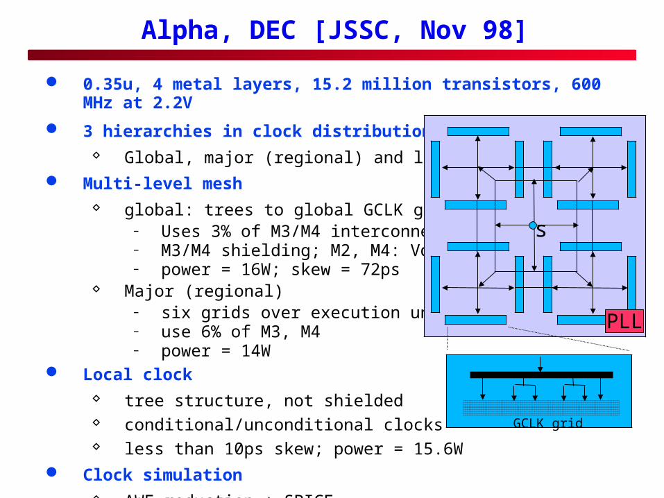
Alpha, DEC [JSSC, Nov 98]

0.35u, 4 metal layers, 15.2 million transistors, 600 MHz at 2.2V

3 hierarchies in clock distribution Global, major (regional) and local

Multi-level mesh global: trees to global GCLK grid

– Uses 3% of M3/M4 interconnect– M3/M4 shielding; M2, M4: Vdd/Vss– power = 16W; skew = 72ps

Major (regional)– six grids over execution units– use 6% of M3, M4– power = 14W

Local clock tree structure, not shielded conditional/unconditional clocks less than 10ps skew; power = 15.6W

Clock simulation AWE-reduction + SPICE

s

PLL

GCLK grid

22

Summary of Processor Clock Design

Three basic routing structures for global clock H-tree

– low skew, smallest routing capacitance, low power– Floorplan flexibility is poor:

Grid or mesh– low skew, increases routing capacitance, worse power– Alpha uses global clock grid and regional clock grids

Spine– Small RC delay because of large spine width– Spine has to balance delays; difficult problem– Routing cap lower than grid but may be higher than H-tree.

Medium

High

Low

Capacitance/Layout area/power

MediumSpine

Medium/highLowGrid

LowLow/mediumH-tree

Floorplan flexibilityClock skewClock structure

High

23

Estimation of Process-dependent Clock Skew in CMOS VLSI, Shoji [JSSC, Oct. 86]

Given two paths from clock source to FFs

Conventional design method

design paths such that skew between S1 and S2 is zero at a (fixed) process corner

However, skew may not be zero at another process corner

Novel idea in the paper

design the two paths such that skew between S1 and S2 is zero for different process corners

TA + TB + TC = TD + TE (typical corner)

For high-current process corner H, TA(H) = TA * 1/fN; TB(H) = TB * 1/fP (fN, fP > 1)

Zero-skew condition at H TA(H) + TB(H) + TC(H) = TD(H) + TE(H) (TA+TC) * 1/fN + TB/FP = TD/fN + TE/fP (TE – TB)/fN = (TE - TB)/fP

CLK

S1 S2

A

B

C

D

E

24

Estimation of Process-dependent Clock Skew in CMOS VLSI, Shoji [JSSC, Oct. 86]

Either TE = TB or fN = fP.

But fN may not be same as fP (for PH-NL process)

In general, TE = TB => TD = TA + TC.

Pull-up and pull-down delays of two paths should be identical.

Determine NMOS & PMOS transistor widths of inverters to achieve this.

Results 1.75 u process Widths selected manually Lead to very small skews at all process corners

Drawbacks only analyzes two paths assumes identical percentage delay variation for

all NMOS (PMOS) devices uses simplistic delay model; ignores wire cap

CLK

S1 S2

A

B

C

D

E

25

Optimal Clock Skew Scheduling

Long & short path constraints impose lower/upper bounds on skew.

long path analysis: aj ai + logic_max + tset_up - Tcycle

short path analysis: aj ai + logic_min - thold

Leads to a set of linear inequalities: ai – a

j c

ij

Given a clock cycle, feasibility can be solved using linear program, more efficiently with Bellman-Ford shortest path [Fishburn TCAD90].

If wish to compute optimum clock cycle, Perform binary search using above feasibility check. Perform parametrized shortest path [Tarjan et al.]

One challenge: realize each ai

Other objectives: minimize power or switching noise.

Logic FF

FF

clk

skew

i j

aiaj

26

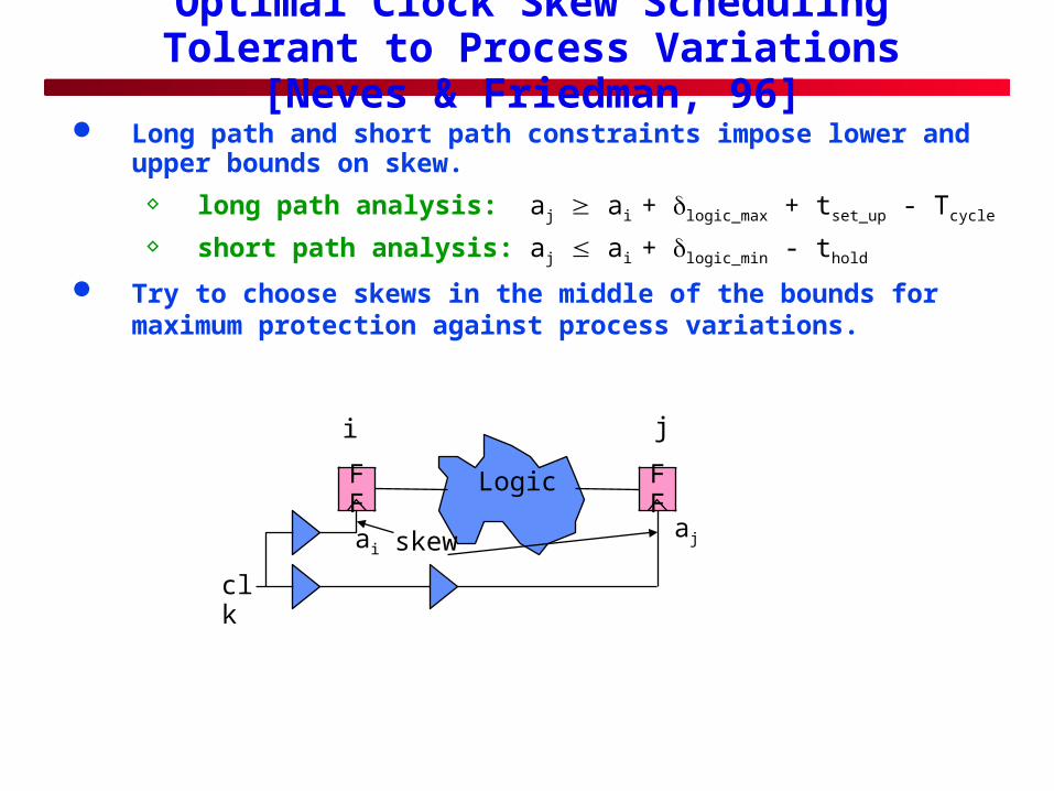
Optimal Clock Skew Scheduling Tolerant to Process Variations [Neves & Friedman, 96]

Long path and short path constraints impose lower and upper bounds on skew.

long path analysis: aj ai + logic_max + tset_up - Tcycle

short path analysis: aj ai + logic_min - thold

Try to choose skews in the middle of the bounds for maximum protection against process variations.

Logic FF

FF

clk

skew

i j

aiaj