1

CHAPTER 7

ATOMIC SPECTRA

7.1 Introduction

Atomic spectroscopy is, of course, a vast subject, and there is no intention in this brief chapter of attempting to cover such a huge field with any degree of completeness, and it is not intended to serve as a formal course in spectroscopy. For such a task a thousand pages would make a good start. The aim, rather, is to summarize some of the words and ideas sufficiently for the occasional needs of the student of stellar atmospheres. For that reason this short chapter has a mere 26 sections. Wavelengths of spectrum lines in the visible region of the spectrum were traditionally expressed in angstrom units (Å) after the nineteenth century Swedish spectroscopist Anders Ångström, one Å being 10−10 m. Today, it is recommended to use nanometres (nm) for visible light or micrometres (µm) for infrared. 1 nm = 10 Å = 10−3 µm= 10−9 m. The older word micron is synonymous with micrometre, and should be avoided, as should the isolated abbreviation µ. The usual symbol for wavelength is λ. Wavenumber is the reciprocal of wavelength; that is, it is the number of waves per metre. The usual symbol is σ, although ν~ is sometimes seen. In SI units, wavenumber would be expressed in m-1, although cm-1 is often used. The extraordinary illiteracy "a line of 15376 wavenumbers" is heard regrettably often. What is intended is presumably "a line of wavenumber 15376 cm-1." The kayser was an unofficial unit formerly seen for wavenumber, equal to 1 cm-1. As some wag once remarked: "The Kaiser (kayser) is dead!" It is customary to quote wavelengths below 200 nm as wavelengths in vacuo, but wavelengths above 200 nm in "standard air". Wavenumbers are usually quoted as wavenumbers in vacuo, whether the wavelength is longer or shorter than 200 nm. Suggestions are made from time to time to abandon this confusing convention; in any case it is incumbent upon any writer who quotes a wavelength or wavenumber to state explicitly whether s/he is referring to a vacuum or to standard air, and not to assume that this will be obvious to the reader. Note that, in using the formula n1λ1 = n2λ2 = n3λ3 used for overlapping orders, the wavelength concerned is neither the vacuum nor the standard air wavelength; rather it is the wavelength in the actual air inside the spectrograph. If I use the symbols λ0 and σ0 for vacuum wavelength and wavenumber and λ and σ for wavelength and wavenumber in standard air, the relation between λ and σ0 is

λσ

=1

0n 7.1.1

"Standard air" is a mythical substance whose refractive index n is given by

2

( ). .. .

.,n − = +

−+

−1 10 834 213

240603 0130

1599 738 9

7

02

02σ σ

7.1.2

where σ0 is in µm-1. This corresponds closely to that of dry air at a pressure of 760 mm Hg and temperature 15o C containing 0.03% by volume of carbon dioxide. To calculate λ given σ0 is straightforward. To calculate σ0 given λ requires iteration. Thus the reader, as an exercise, should try to calculate the vacuum wavenumber of a line of standard air wavelength 555.5 nm. In any case, the reader who expects to be dealing with wavelengths and wavenumbers fairly often should write a small computer or calculator program that allows the calculation to go either way. Frequency is the number of waves per second, and is expressed in hertz (Hz) or MHz or GHz, as appropriate. The usual symbol is ν, although f is also seen. Although wavelength and wavenumber change as light moves from one medium to another, frequency does not. The relation between frequency, speed and wavelength is c = νλ0, 7.1.3 where c is the speed in vacuo, which has the defined value 2.997 924 58 % 108 m s-1. A spectrum line results from a transition between two energy levels of an atom The frequency of the radiation involved is related to the difference in energy levels by the familiar relation hν = ∆E, 7.1.4 where h is Planck's constant, 6.626075 % 10-34 J s. If the energy levels are expressed in joules, this will give the frequency in Hz. This is not how it is usually done, however. What is usually tabulated in energy level tables is E hc/ ( ) , in units of cm-1. This quantity is known as the term

value T of the level. Equation 7.1.4 then becomes σ0 = ∆T. 7.1.5 Thus the vacuum wavenumber is simply the difference between the two tabulated term values. In some contexts it may also be convenient to express energy levels in electron volts, 1 eV being 1.60217733 % 10-19 J. Energy levels of neutral atoms are typically of the order of a few eV. The energy required to ionize an atom from its ground level is called the ionization energy, and its SI unit would be the joule. However, one usually quotes the ionization energy in eV, or the ionization potential in volts. It may be remarked that sometimes one hears the process of formation of a spectrum line as one in which an "electron" jumps from one energy level to another. This is quite wrong. It is true that there is an adjustment of the way in which the electrons are distributed around the atomic

3

nucleus, but what is tabulated in tables of atomic energy levels or drawn in energy level diagrams is the energy of the atom, and in equation 7.1.4 ∆E is the change in energy of the atom.

This includes the kinetic energy of all the particles in the atom as well as the mutual potential energy between the particles. We have seen that the wavenumber of a line is equal to the difference between the term values of the two levels involved in its formation. Thus, if we know the term values of two levels, it is a trivial matter to calculate the wavenumber of the line connecting them. In spectroscopic analysis the problem is very often the converse - you have measured the wavenumbers of several spectrum lines; can you from these calculate the term values of the levels involved? For example, here are four (entirely hypothetical and artificially concocted for this problem) vacuum wavenumbers, in µm-1:

1.96643 2.11741 2.28629 2.43727

The reader who is interested on spectroscopy, or in crossword puzzles or jigsaw puzzles, is very strongly urged to calculate the term values of the four levels involved with these lines, and to see whether this can or cannot be done without ambiguity from these data alone. Of course, you may object that there are six ways in which four levels can be joined in pairs, and therefore I should have given you the wavenumbers of six lines. Well, sorry to be unsympathetic, but perhaps two of the lines are two faint to be seen, or they may be forbidden by selection rules, or their wavelengths might be out of the range covered by your instrument. In any case, I have told you that four levels are involved, which is more information that you would have if you had just measured the wavenumbers of these lines from a spectrum that you had obtained in the laboratory. And at least I have helped by converting standard air wavelengths to vacuum wavenumbers. The exercise will give some appreciation of some of the difficulties in spectroscopic analysis. In the early days of spectroscopy, in addition to flames and discharge tubes, common spectroscopic sources included arcs and sparks. In an arc, two electrodes with a hundred or so volts across them are touched, and then drawn apart, and an arc forms. In a spark, the potential difference across the electrodes is some thousands of volts, and it is not necessary to touch the electrodes together; rather, the electrical insulation of the air breaks down and a spark flies from one electrode to the other. It was noticed that the arc spectrum was usually very different from the spark spectrum, the former often being referred to as the "first" spectrum and the latter as the "second" spectrum. If the electrodes were, for example, of carbon, the arc or first spectrum would be denoted by C I and the spark or second spectrum by C II. It has long been known now that the "first" spectrum is mostly that of the neutral atom, and the "second" spectrum mostly that of the singly-charged ion. Since the atom and the ion have different electronic structures, the two spectra are very different. Today, we use the symbols C I , or Fe I, or Zr I , etc., to denote the spectrum of the neutral atom, regardless of the source, and C II , C III , C IV , etc., to denote the spectra of the singly-, doubly- triply-ionized atoms, C+ , C++ , C+++ , etc. There are 4278

4

possible spectra of the first 92 elements to investigate, and many more if one adds the transuranic elements, so there is no want of spectra to study. Hydrogen, of course, has only one spectrum, denoted by H I, since ionized hydrogen is merely a proton. The regions in space where hydrogen is mostly ionized are known to astronomers as "H II regions". Strictly, this is a misnomer, for there is no "second spectrum" of hydrogen, and a better term would be "H+ regions", but the term "H II regions" is by now so firmly entrenched that it is unlikely to change. It is particularly ironic that the spectrum exhibited by an "H II region" is that of neutral hydrogen (e.g. the well-known Balmer series), as electrons and protons recombine and drop down the energy level ladder. On the other hand, apart from the 21 cm line in the radio region, the excitation temperature in regions where hydrogen is mostly neutral (and hence called, equally wrongly, "H I regions") is far too low to show the typical spectrum of neutral hydrogen, such as the Balmer series. Thus it can be accurately said that "H II regions" show the spectrum of H I, and "H I regions" do not. Lest it be thought that this is unnecessary pedantry, it should be made clear at the outset that the science of spectroscopy, like those of celestial mechanics or quantum mechanics, is one in which meticulous accuracy and precision of ideas is an absolute necessity, and there is no room for vagueness, imprecision, or improper usage of terms. Those who would venture into spectroscopy would do well to note this from the beginning. 7.2 A Very Brief History of Spectroscopy

Perhaps the first quantitative investigation that can be said to have a direct bearing on the science of spectroscopy would be the discovery of Snel's law of refraction in about 1621. I am not certain, but I believe the original spelling of the Dutch mathematician who discovered the law was Willebrod Snel or Willebrord Snel, whose name was latinized in accordance with the custom of learned scholars of the day to Snellius, and later anglicized to the more familiar spelling Snell. Sir Isaac Newton's experiments were described in his Opticks of 1704. A most attractive illustration of the experiment, described in a work by Voltaire, is reproduced in Condon and Shortly's famous Theory of Atomic Spectra (1935). Newton showed that sunlight is dispersed by a prism into a band of colours, and the colours are recombined into white light when passed through an oppositely-oriented second prism. The infrared spectrum was discovered by Sir William Herschel in 1800 by placing thermometers beyond the red end of the visible spectrum. Johann Ritter the following year (and independently Wollaston) discovered the ultraviolet spectrum. In the period 1800-1803 Thomas Young demonstrated the wave nature of light with his famous double slit experiment, and he correctly explained the colours of thin films using the undulatory theory. Using Newton's measurements of this phenomenon, Young computed the wavelengths of Newton's seven colours and obtained the range 424 to 675 nm. In 1802 William Wollaston discovered dark lines in the solar spectrum, but attached little significance to them. In 1814 Joseph Fraunhofer, a superb instrument maker, made a detailed examination of the solar spectrum; he made a map of 700 of the lines we now refer to as "Fraunhofer lines". (Spectrum lines in general are sometimes described as "Fraunhofer lines", but the term should

5

correctly be restricted to the dark lines in the solar spectrum.) In 1817 he observed the first stellar spectra with an objective prism. He noted that planetary spectra resembled the solar spectrum, while many stellar spectra differed. Although the phenomenon of diffraction had been described as early as 1665 by Grimaldi, and Young had explained double-slit diffraction, Fraunhofer constructed the first diffraction grating by winding wires on two finely-cut parallel screws. With these gratings he measured the first wavelengths of spectrum lines, obtaining 588.7 for the line he had labelled D. We now know that this line is a close pair of lines of Na I, whose modern wavelengths are 589.0 and 589.6 nm. That different chemical elements produce their own characteristic spectra was noted by several investigators, including Sir John Herschel, (son of Sir William), Fox Talbot (pioneer in photography), Sir Charles Wheatstone (of Wheatstone Bridge fame), Anders Ångström (after whom the now obsolete unit the angstrom, Å, was named), and Jean Bernard Foucault (famous for his pendulum but also for many important studies in physical optics, including the speed of light) and especially by Kirchhoff and Bunsen. The fundamental quantitative law known as Kirchhoff's Law (see Chapter 2, section 2.4) was announced in 1859, and Kirchhoff and Bunsen conducted their extensive examination of the spectra of several elements. They correctly explained the origin of the solar Fraunhofer lines, investigated the chemical composition of the solar atmosphere, and laid the basic foundations of spectrochemical analysis. In 1868 Ångström published wavelengths of about 1000 solar Fraunhofer lines. In the 1870s, Rowland started to produce diffraction gratings of unparalleled quality and published extensive lists of solar wavelengths. New elements were being discovered spectroscopically: Cs, Rb, Tl (1860-61); In (1863); He (1868 - in the chromosphere of the solar spectrum at the instants of second and third contact of a solar eclipse, by Lockyer); Ga (1875); Tm (1870); Nd, Pr (1885); Sm, Ho (1886); Lu, Yb (1907). Michelson measured the wavelength of three Cd I lines with great precision in 1893, and Fabry and Pérot measured the wavelengths of other lines in terms of the Cd I standards. For many years the wavelength of a cadmium lines was used as a basis for the definition of the metre. Although the existence of ultraviolet radiation had been detected by Richter, the first person actually to see an ultraviolet (UV) spectrum was Sir George Stokes (of viscosity and fluorescence fame), using a quartz prism (ordinary glass absorbs UV) and a fluorescent uranium phosphate screen. In 1906 Lyman made extensive investigations into ultraviolet spectra, including the hydrogen series now known as the Lyman series. Langley invented the bolometer in 1881, paving the way to the investigation of infrared spectra by Paschen. Balmer published his well-known formula for the wavelengths of the hydrogen Balmer series in 1885. Zeeman discovered magnetic splitting in 1896. Bohr's theory of the hydrogen atom appeared in 1913, and the wave mechanics of Schrödinger was developed in the mid 1920s.

6

7.3 The Hydrogen Spectrum

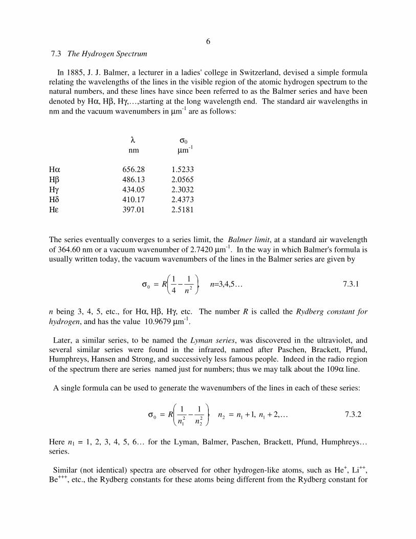
In 1885, J. J. Balmer, a lecturer in a ladies' college in Switzerland, devised a simple formula relating the wavelengths of the lines in the visible region of the atomic hydrogen spectrum to the natural numbers, and these lines have since been referred to as the Balmer series and have been denoted by Hα, Hβ, Hγ,…,starting at the long wavelength end. The standard air wavelengths in nm and the vacuum wavenumbers in µm-1 are as follows:

λ σ0 nm µm-1 Hα 656.28 1.5233

Ηβ 486.13 2.0565

Ηγ 434.05 2.3032

Ηδ 410.17 2.4373

Ηε 397.01 2.5181

The series eventually converges to a series limit, the Balmer limit, at a standard air wavelength of 364.60 nm or a vacuum wavenumber of 2.7420 µm-1. In the way in which Balmer's formula is usually written today, the vacuum wavenumbers of the lines in the Balmer series are given by

K5,4,3,1

41

20 =

−=σ n

nR 7.3.1

n being 3, 4, 5, etc., for Hα, Hβ, Hγ, etc. The number R is called the Rydberg constant for

hydrogen, and has the value 10.9679 µm-1. Later, a similar series, to be named the Lyman series, was discovered in the ultraviolet, and several similar series were found in the infrared, named after Paschen, Brackett, Pfund, Humphreys, Hansen and Strong, and successively less famous people. Indeed in the radio region of the spectrum there are series named just for numbers; thus we may talk about the 109α line. A single formula can be used to generate the wavenumbers of the lines in each of these series:

K,2,1,111122

221

0 ++=

−=σ nnn

nnR 7.3.2

Here n1 = 1, 2, 3, 4, 5, 6… for the Lyman, Balmer, Paschen, Brackett, Pfund, Humphreys… series. Similar (not identical) spectra are observed for other hydrogen-like atoms, such as He+, Li++, Be+++, etc., the Rydberg constants for these atoms being different from the Rydberg constant for

7

hydrogen. Deuterium and tritium have very similar spectra and their Rydberg constants are very close to that of the 1H atom. Each "line" of the hydrogen spectrum, in fact, has fine structure, which is not easily seen and usually needs carefully designed experiments to observe it. This fine structure need not trouble us at present, but we shall later be obliged to consider it. An interesting historical story connected with the fine structure of hydrogen is that the quantity ( )ce h0

2 4/ πε plays a prominent role in the theory that describes it. This quantity, which is a dimensionless pure number, is called the fine structure constant α, and the reciprocal of its value is close to the prime number 137. Sir Arthur Eddington, one of the greatest figures in astrophysics in the early twentieth century, had an interest in possible connections between the fundamental constants of physics and the natural numbers, and became almost obsessed with the notion that the reciprocal of the fine structure constant should be exactly 137, even insisting on hanging his hat on a conference hall coatpeg number 137. 7.4 The Bohr Model of Hydrogen-like Atoms

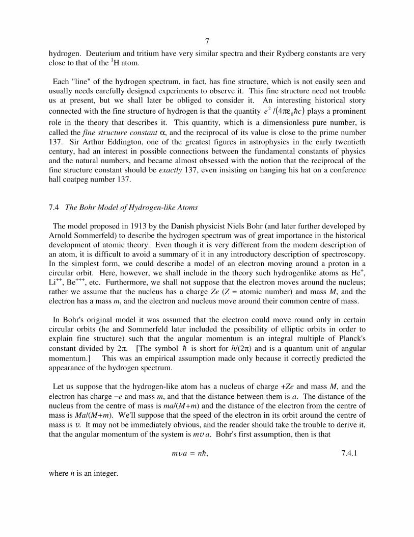
The model proposed in 1913 by the Danish physicist Niels Bohr (and later further developed by Arnold Sommerfeld) to describe the hydrogen spectrum was of great importance in the historical development of atomic theory. Even though it is very different from the modern description of an atom, it is difficult to avoid a summary of it in any introductory description of spectroscopy. In the simplest form, we could describe a model of an electron moving around a proton in a circular orbit. Here, however, we shall include in the theory such hydrogenlike atoms as He+, Li++, Be+++, etc. Furthermore, we shall not suppose that the electron moves around the nucleus; rather we assume that the nucleus has a charge Ze (Z = atomic number) and mass M, and the electron has a mass m, and the electron and nucleus move around their common centre of mass. In Bohr's original model it was assumed that the electron could move round only in certain circular orbits (he and Sommerfeld later included the possibility of elliptic orbits in order to explain fine structure) such that the angular momentum is an integral multiple of Planck's constant divided by 2π. [The symbol h is short for h/(2π) and is a quantum unit of angular momentum.] This was an empirical assumption made only because it correctly predicted the appearance of the hydrogen spectrum. Let us suppose that the hydrogen-like atom has a nucleus of charge +Ze and mass M, and the electron has charge −e and mass m, and that the distance between them is a. The distance of the nucleus from the centre of mass is ma/(M+m) and the distance of the electron from the centre of mass is Ma/(M+m). We'll suppose that the speed of the electron in its orbit around the centre of mass is v. It may not be immediately obvious, and the reader should take the trouble to derive it, that the angular momentum of the system is mv a. Bohr's first assumption, then is that ,hnam =v 7.4.1 where n is an integer.

8

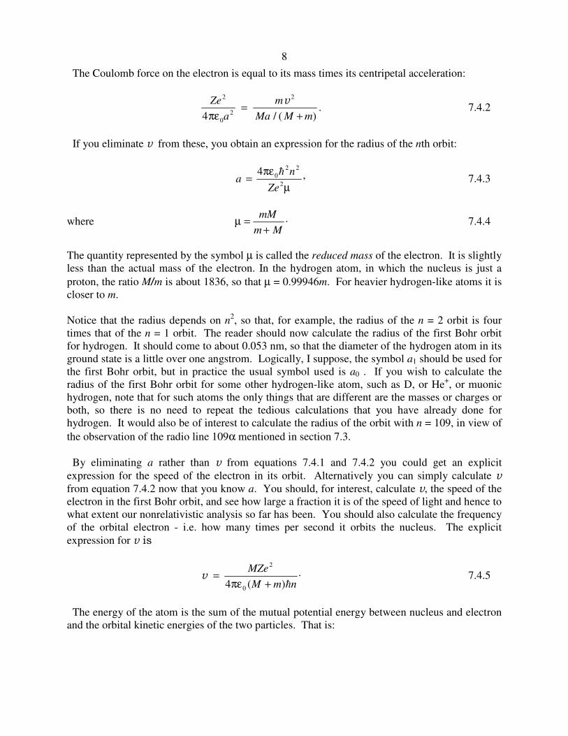
The Coulomb force on the electron is equal to its mass times its centripetal acceleration:

Ze

a

m

Ma M m

2

02

2

4πε=

+

v

/ ( ). 7.4.2

If you eliminate v from these, you obtain an expression for the radius of the nth orbit:

,42

220

µ

επ=

Ze

na

h 7.4.3

where µ =+

mM

m M. 7.4.4

The quantity represented by the symbol µ is called the reduced mass of the electron. It is slightly less than the actual mass of the electron. In the hydrogen atom, in which the nucleus is just a proton, the ratio M/m is about 1836, so that µ = 0.99946m. For heavier hydrogen-like atoms it is closer to m. Notice that the radius depends on n2, so that, for example, the radius of the n = 2 orbit is four times that of the n = 1 orbit. The reader should now calculate the radius of the first Bohr orbit for hydrogen. It should come to about 0.053 nm, so that the diameter of the hydrogen atom in its ground state is a little over one angstrom. Logically, I suppose, the symbol a1 should be used for the first Bohr orbit, but in practice the usual symbol used is a0 . If you wish to calculate the radius of the first Bohr orbit for some other hydrogen-like atom, such as D, or He+, or muonic hydrogen, note that for such atoms the only things that are different are the masses or charges or both, so there is no need to repeat the tedious calculations that you have already done for hydrogen. It would also be of interest to calculate the radius of the orbit with n = 109, in view of the observation of the radio line 109α mentioned in section 7.3. By eliminating a rather than v from equations 7.4.1 and 7.4.2 you could get an explicit expression for the speed of the electron in its orbit. Alternatively you can simply calculate v from equation 7.4.2 now that you know a. You should, for interest, calculate v, the speed of the electron in the first Bohr orbit, and see how large a fraction it is of the speed of light and hence to what extent our nonrelativistic analysis so far has been. You should also calculate the frequency of the orbital electron - i.e. how many times per second it orbits the nucleus. The explicit expression for v is

.)(4 0

2

nmM

MZe

h+επ=v 7.4.5

The energy of the atom is the sum of the mutual potential energy between nucleus and electron and the orbital kinetic energies of the two particles. That is:

9

.4

2

212

21

0

2

++

επ−=

M

mMm

a

ZeE

vv 7.4.6

If we make use of equation 7.4.2 this becomes

.

)(

221

22

212

21

2

v

vvv

+−=

+++

−=

M

mMm

M

mm

M

mMmE

Then, making use of equation 7.4.5, we obtain for the energy

( )

.1.42 222

0

42

n

eZE

hεπ

µ−= 7.4.7

In deriving this expression for the energy, we had taken the potential energy to be zero at infinite separation of proton and nucleus, which is a frequent convention in electrostatics. That is, the energy level we have calculated for a bound orbit is expressed relative to the energy of ionized hydrogen. Hence the energy of all bound orbits is negative. In tables of atomic energy levels, however, it is more usual to take the energy of the ground state (n=1) to be zero. In that case the energy levels are given by

( )

.11.

42 2220

42

−

επ

µ=

n

eZE

h 7.4.8

Further, as explained in section 7.1, it is customary to tabulate term values T rather than energy levels, and this is achieved by dividing by hc. Thus

( )

.1

1.42 222

0

42

−

επ

µ=

nhc

eZT

h 7.4.9

The expression before the large parentheses is called the Rydberg constant for the atom in question. For hydrogen (1H : Z = 1), it has the value 1.09679 × 107 m-1. If we put Z = 1 and µ = m the resulting expression is called the Rydberg constant for a

hydrogen nucleus of infinite mass; it is the expression one would arrive at if one neglected the motion of the nucleus. It is one of the physical constants whose value is known with greatest precision, its value being R∞ = 1.097 373 153 4 × 107 m-1. (The gravitational constant G is probably the least precisely known.)

10

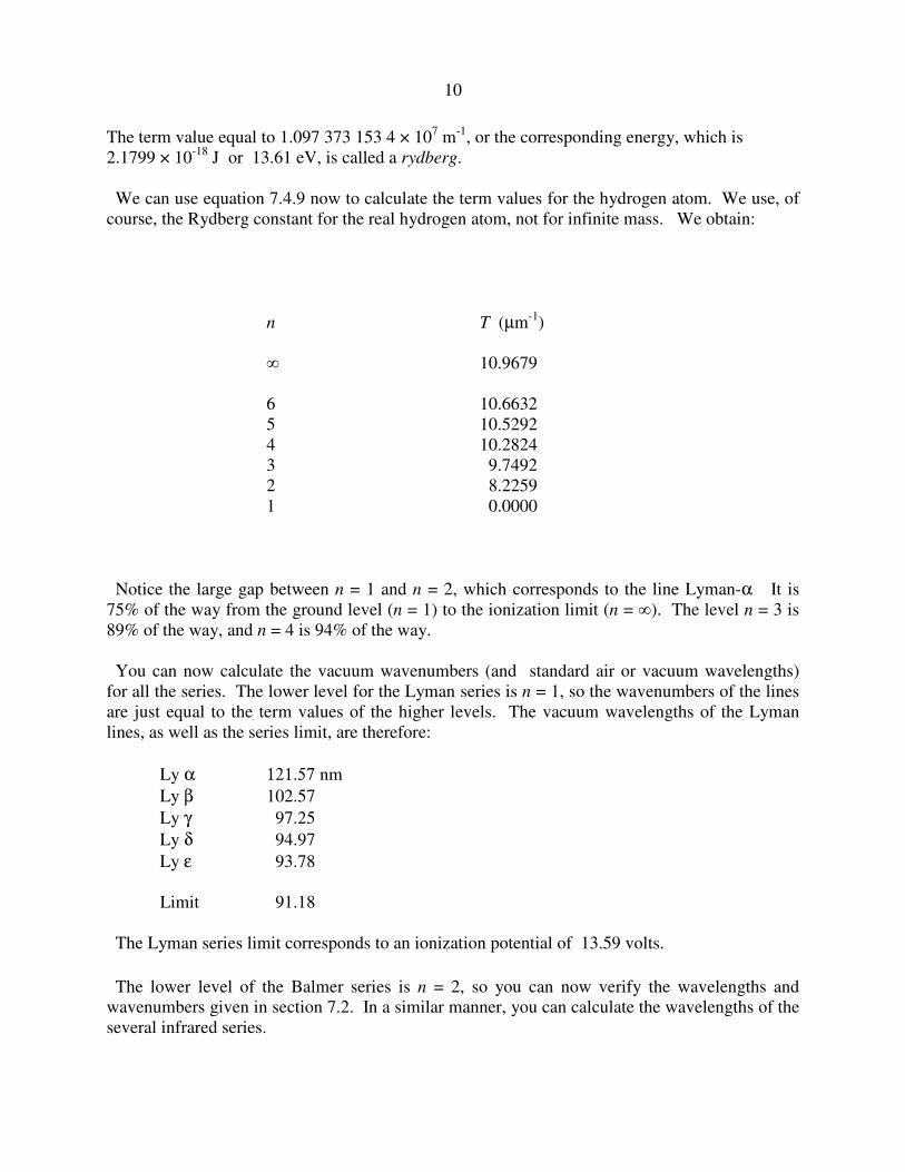
The term value equal to 1.097 373 153 4 × 107 m-1, or the corresponding energy, which is 2.1799 × 10-18 J or 13.61 eV, is called a rydberg. We can use equation 7.4.9 now to calculate the term values for the hydrogen atom. We use, of course, the Rydberg constant for the real hydrogen atom, not for infinite mass. We obtain: n T (µm-1)

∞ 10.9679

6 10.6632 5 10.5292 4 10.2824 3 9.7492 2 8.2259 1 0.0000

Notice the large gap between n = 1 and n = 2, which corresponds to the line Lyman-α It is 75% of the way from the ground level (n = 1) to the ionization limit (n = ∞). The level n = 3 is 89% of the way, and n = 4 is 94% of the way. You can now calculate the vacuum wavenumbers (and standard air or vacuum wavelengths) for all the series. The lower level for the Lyman series is n = 1, so the wavenumbers of the lines are just equal to the term values of the higher levels. The vacuum wavelengths of the Lyman lines, as well as the series limit, are therefore: Ly α 121.57 nm Ly β 102.57 Ly γ 97.25 Ly δ 94.97 Ly ε 93.78 Limit 91.18 The Lyman series limit corresponds to an ionization potential of 13.59 volts. The lower level of the Balmer series is n = 2, so you can now verify the wavelengths and wavenumbers given in section 7.2. In a similar manner, you can calculate the wavelengths of the several infrared series.

11

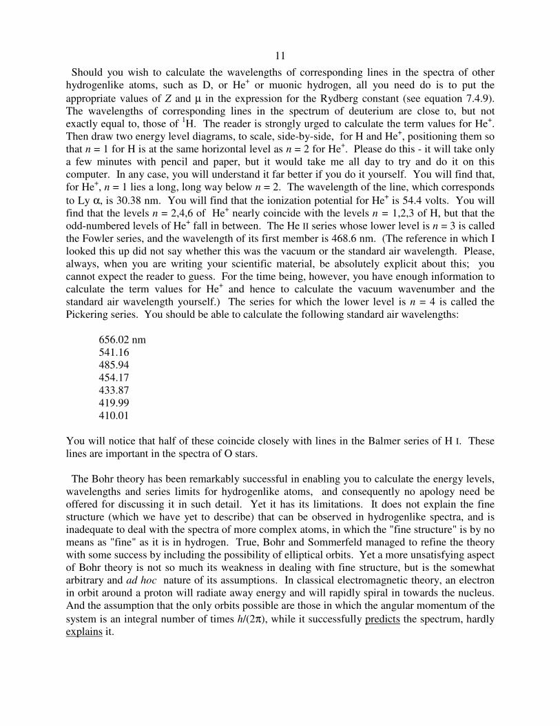
Should you wish to calculate the wavelengths of corresponding lines in the spectra of other hydrogenlike atoms, such as D, or He+ or muonic hydrogen, all you need do is to put the appropriate values of Z and µ in the expression for the Rydberg constant (see equation 7.4.9). The wavelengths of corresponding lines in the spectrum of deuterium are close to, but not exactly equal to, those of 1H. The reader is strongly urged to calculate the term values for He+. Then draw two energy level diagrams, to scale, side-by-side, for H and He+, positioning them so that n = 1 for H is at the same horizontal level as n = 2 for He+. Please do this - it will take only a few minutes with pencil and paper, but it would take me all day to try and do it on this computer. In any case, you will understand it far better if you do it yourself. You will find that, for He+, n = 1 lies a long, long way below n = 2. The wavelength of the line, which corresponds to Ly α, is 30.38 nm. You will find that the ionization potential for He+ is 54.4 volts. You will find that the levels n = 2,4,6 of He+ nearly coincide with the levels n = 1,2,3 of H, but that the odd-numbered levels of He+ fall in between. The He II series whose lower level is n = 3 is called the Fowler series, and the wavelength of its first member is 468.6 nm. (The reference in which I looked this up did not say whether this was the vacuum or the standard air wavelength. Please, always, when you are writing your scientific material, be absolutely explicit about this; you cannot expect the reader to guess. For the time being, however, you have enough information to calculate the term values for He+ and hence to calculate the vacuum wavenumber and the standard air wavelength yourself.) The series for which the lower level is n = 4 is called the Pickering series. You should be able to calculate the following standard air wavelengths: 656.02 nm 541.16 485.94 454.17 433.87 419.99 410.01 You will notice that half of these coincide closely with lines in the Balmer series of H I. These lines are important in the spectra of O stars. The Bohr theory has been remarkably successful in enabling you to calculate the energy levels, wavelengths and series limits for hydrogenlike atoms, and consequently no apology need be offered for discussing it in such detail. Yet it has its limitations. It does not explain the fine structure (which we have yet to describe) that can be observed in hydrogenlike spectra, and is inadequate to deal with the spectra of more complex atoms, in which the "fine structure" is by no means as "fine" as it is in hydrogen. True, Bohr and Sommerfeld managed to refine the theory with some success by including the possibility of elliptical orbits. Yet a more unsatisfying aspect of Bohr theory is not so much its weakness in dealing with fine structure, but is the somewhat arbitrary and ad hoc nature of its assumptions. In classical electromagnetic theory, an electron in orbit around a proton will radiate away energy and will rapidly spiral in towards the nucleus. And the assumption that the only orbits possible are those in which the angular momentum of the system is an integral number of times h/(2π), while it successfully predicts the spectrum, hardly explains it.

12

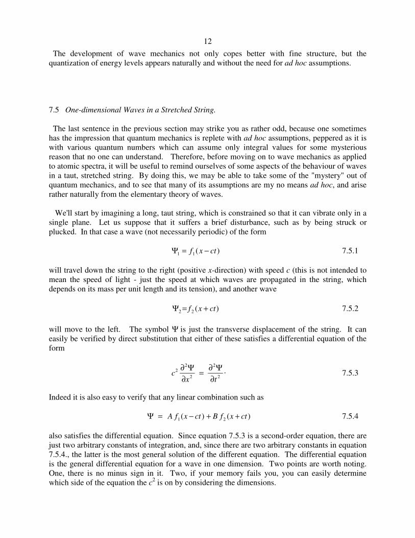
The development of wave mechanics not only copes better with fine structure, but the quantization of energy levels appears naturally and without the need for ad hoc assumptions. 7.5 One-dimensional Waves in a Stretched String. The last sentence in the previous section may strike you as rather odd, because one sometimes has the impression that quantum mechanics is replete with ad hoc assumptions, peppered as it is with various quantum numbers which can assume only integral values for some mysterious reason that no one can understand. Therefore, before moving on to wave mechanics as applied to atomic spectra, it will be useful to remind ourselves of some aspects of the behaviour of waves in a taut, stretched string. By doing this, we may be able to take some of the "mystery" out of quantum mechanics, and to see that many of its assumptions are my no means ad hoc, and arise rather naturally from the elementary theory of waves. We'll start by imagining a long, taut string, which is constrained so that it can vibrate only in a single plane. Let us suppose that it suffers a brief disturbance, such as by being struck or plucked. In that case a wave (not necessarily periodic) of the form Ψ1 1= −f x ct( ) 7.5.1 will travel down the string to the right (positive x-direction) with speed c (this is not intended to mean the speed of light - just the speed at which waves are propagated in the string, which depends on its mass per unit length and its tension), and another wave )(22 ctxf +=Ψ 7.5.2 will move to the left. The symbol Ψ is just the transverse displacement of the string. It can easily be verified by direct substitution that either of these satisfies a differential equation of the form

cx t

22

2

2

2

∂

∂

∂

∂

Ψ Ψ= . 7.5.3

Indeed it is also easy to verify that any linear combination such as Ψ = − + +A f x ct B f x ct1 2( ) ( ) 7.5.4 also satisfies the differential equation. Since equation 7.5.3 is a second-order equation, there are just two arbitrary constants of integration, and, since there are two arbitrary constants in equation 7.5.4., the latter is the most general solution of the different equation. The differential equation is the general differential equation for a wave in one dimension. Two points are worth noting. One, there is no minus sign in it. Two, if your memory fails you, you can easily determine which side of the equation the c2 is on by considering the dimensions.

13

If the function is periodic, it can be represented as the sum of a number (perhaps an infinite number) of sine and cosine terms with frequencies related to each other by rational fractions. Even if the function is not periodic, it can still be represented by sine and cosine functions, except that in this case there is a continuous distribution of component frequencies. The distribution of component frequencies is then the Fourier transform of the wave profile. (If you are shaky with Fourier transforms, do not worry - I promise not to mention them again in this chapter.) Because of this, I shall assume all waves to be sinusoidal functions. Let us now assume that the string is fixed at both ends. (Until this point I had not mentioned whether the ends of the string were fixed or not, although I had said that the string was taut. I suppose it would be possible for those of mathematical bent to imagine a taut string of infinite length, though my imagination begins to falter after the first few parsecs.) If a sine wave travels down the string, when it reaches the end it reverses its direction, and it does so again at the other end. What happens is that you end up with two waves travelling in opposite directions:

Ψ = − + +

= − + +

a k x ct a k x ct

a kx t a kx t

sin ( ) sin ( )

sin( ) sin ( ).ω ω 7.5.5

Here k is the propagation constant 2π/λ and ω is the angular frequency 2πν. By a trigonometric identity this can be written: Ψ = 2a t kxcos sin .ω 7.5.6 This is a stationary sin wave (sin kx) whose amplitude (2a cos ωt) varies periodically with time. In other words, it is a stationary or standing wave system. Notice particularly that a stationary or standing wave system is represented by the product of a function of space and a function of time: Ψ( , ) ( ). ( ).x t x t= ψ χ 7.5.7 Because the string is fixed at both ends (these are fixed boundary conditions) the only possible wavelengths are such that there is a node at each fixed end, and consequently there can only be an integral number of antinodes or half wavelengths along the length of the string. If the length of the string is l, the fundamental mode of vibration has a wavelength 2l and a fundamental frequency of c/(2l). Other modes (the higher harmonics) are equal to an integral number of times this fundamental frequency; that is nc/(2l), where n is an integer. Note that the introduction of this number n, which is restricted to integral values (a "quantum number", if you will) is a consequence of the fixed boundary conditions. Which modes are excited and with what relative amplitudes depends upon the initial conditions − that is, on whether the string is plucked (initially 0,0 =Ψ≠Ψ & ) or struck (initially

0,0 ≠Ψ=Ψ & ), and where it was plucked or struck. It would require some skill and practice (ask any musician) to excite only one vibrational mode, unless you managed to get the initial conditions exactly right, and the general motion is a linear superposition of the normal modes.

14

I'll mention just one more thing here, which you should recall if you have studied waves at all, namely that the energy of a wave of a given frequency is proportional to the square of its amplitude. Volumes could be written about the vibrations of a stretched string. I would ask the reader to take notice especially of these four points.

1. A stationary solution is the product of a function of space and a function of time.

2. Restriction to a discrete set of frequencies involving an integral number is a consequence of fixed boundary conditions.

3. The general motion is a linear combination of the normal modes.

4. The energy of a wave is proportional to the square of its amplitude.

7.6 Vibrations of a Uniform Sphere.

This is a three-dimensional problem and the wave equation is .22 Ψ=Ψ∇ &&c 7.6.1 The wave-function here, Ψ, which is a function of the coordinates and the time, can be thought of as the density of the sphere; it describes how the density of the sphere is varying in space and with time. In problems of spherical symmetry it is convenient to write this in spherical coordinates. The expression for ∇2 in spherical coordinates is fairly lengthy. You have probably not memorized it, but you will have seen it or know where to look it up. Stationary solutions are of the form ( ) ( ) ( )..,,;,, trtr χφθψ=φθΨ 7.6.2 Is it necessary to know the mathematical details of these functions? Probably not if it is not your intention to have a career in theoretical spectroscopy. If you are going to have a career in theoretical spectroscopy, it probably wouldn't hurt to do the detailed calculation - but in practice a great deal of calculation can be and is done without reference to the detailed algebra; all that is necessary to know and become familiar with are the properties of the functions and how they react to the several operators encountered in quantum mechanics. At this stage, we are just looking at some general principles, and need not worry about the details of the algebra, which can be fairly involved. The spherical coordinates r, θ, φ are independent variables, and consequently the time-independent part of the wave function can be written as the product of three functions:

15

ψ θ φ θ φ( , , ) ( ). ( ). ( ).r R r= Θ Φ 7.6.3 Again, it is not immediately necessary to know the detailed forms of these functions - you will find them in various books on physics or chemistry or spectroscopy. The simplest is Φ − it is a simple sinusoidal function, usually written as e

im− φ . The function Θ is a bit more complicated and it involves things called Legendre polynomials. The function R involves somewhat less-familiar polynomials called Laguerre polynomials. But there are boundary conditions. Thus φ goes only from 0 to 2π, and in that interval there can only be an integral number of half waves. Likewise, θ goes only from 0 to π, and r goes only from 0 to a, where a is the radius of the sphere. All three of these functions have integral "quantum numbers" associated with them. There is nothing mysterious about this, nor is it necessary to see the detailed algebra to see why this must be so; it is one of the inevitable constraints of fixed boundary conditions. The function R, the radial part of the wavefunction, has associated with it an integer n , which can take only integral values 1, 2. 3,… . The function Θ, the meridional wavefunction, has associated with it an integer l, which, for a given radial function (i.e. a given value of n) can have only the n different integral values 0, 1, 2, … …n−1. Finally, the function Φ, the azimuthal wavefunction, has associated with it an integer m, which, for a given meridional function (i.e. a given value of l) can have only the 2l+1 different integral values −l, −l+1, … 0, …l−1, l. Thus for a given n, the number of possible wavefunctions is

2 10

1

ln

+−

∑ .

You will have to remember how to sum arithmetic series in order to evaluate this, so please do so. The answer is n2. When I first came across these quantum numbers, it was in connection with the wave mechanics of the hydrogen atom, and I thought there was something very mysterious about atomic physics. I was reassured only rather later - as I hope you will be reassured now - that the introduction of these quantum numbers is nothing to do with some special mysterious properties of atoms, but comes quite naturally out of the classical theory of vibrating spheres. Indeed, if you come to think about it, it would be very difficult indeed to believe that the wavefunctions of vibrating spheres did not involve numbers that had to be integers with restrictions on them. The time-independent part of the wavefunction can be written: ( ) )().().(,, φΦθΘ=φθψ mlmnllmn rRr . 7.6.4 Often the angular parts of the wavefunction are combined into a single function: Ylm lm m( , ) ( ). ( ).θ φ θ φ= Θ Φ 7.6.5 The functions Ylm are known as spherical harmonics.

16

When performing various manipulations on the wavefunctions, very often all that happens is that you end up with a similar function but with different values of the integers ("quantum numbers"). Anyone who does a lot of such calculations soon gets used to this, and consequently, rather than write out the rather lengthy functions in full, what is done is merely to list the quantum number of a function between two special symbols known as a "ket". (That's one half of a bracket.) Thus a wavefunction may be written merely as |lmn>. This is done frequently in the quantum mechanics of atoms. I have never seen it done in other, more "classical" branches of physics, but I see no reason why it should not be done, and I dare say that it is in some circles. The problem of a vibrating sphere of uniform density is fairly straightforward. Similar problems face geophysicists or planetary scientists when discussing the interiors of the Earth or the Moon or other planets, or astrophysicists studying "helioseismology" or "asteroseismology" - except that you have to remember there that you are not dealing with uniform spheres. 7.7 The Wave Nature of the Electron.

In 1906 Barkla had shown that when "soft" (relatively long wavelength, low-energy) x-rays were scattered by carbon, they exhibited polarization phenomena in just the way one would expect if they were transverse waves. In 1913 the father-and-son team of W.H and W.L. Bragg had performed their experiments on the diffraction and interference of x-rays by crystals, and they showed that x-rays behaved just as one would expect for short wavelength electromagnetic waves. In 1919, Compton carried out his famous experiments on the scattering of x-rays by light atoms, including carbon, though he used higher energy ("harder") x-rays than in Barkla's experiments. Some of the x-rays were scattered without change of wavelength, as expected from classical Thomson scattering theory, and the wave nature of x-rays appeared to be very firmly established. Yet not all of the x-rays were scattered thus. Indeed when the scattering was from a light element such as carbon most of the scattered x-rays were found to have a longer wavelength than the incident x-rays. Most readers will be familiar with at least the broad outline of these experiments, and how Compton showed that the phenomenon could most easily be explained if, instead of being treated as waves of wavelength λ, they were treated as though they were particles of momentum h/λ. Thus x-rays appeared to have a "wave-particle duality", their behaviour in some circumstances being better treated as a wave phenomenon, and in others as though they were particles. In 1924 de Broglie speculated that perhaps the electron, hitherto regarded, following the initial experiments in 1897 of J. J. Thomson, as a particle, might also exhibit "wave-particle duality" and in some circumstances, rather than be treated as a particle of momentum p might better be described as a wave of wavelength ph / . During the 1920s Davisson and Germer indeed did scattering experiments, in which electrons were scattered from a nickel crystal, and they found that electrons were selectively scattered in a particular direction just as they would if they were waves, and in a rather similar manner to the Bragg scattering of x-rays. Thus indeed it seemed that electrons, while in some circumstances behaving like particles, in others behaved like waves.

17

De Broglie went further and suggested that, if electrons could be described as waves, then perhaps in a Bohr circular orbit, the electron waves formed a standing wave system with an integral number of waves around the orbit: nλ = 2π r. 7.7.1 Then, if λ = h/(mv), we have mv r = nh/(2π), 7.7.2 thus neatly "explaining" Bohr's otherwise ad hoc assumption, described by equation 7.4.1. From a modern point of view this "explanation" may look somewhat quaint, and little less "ad hoc" than Bohr's original assumption. One might also think that perhaps there should have been an integral number of half-wavelengths in a Bohr orbit. Yet it portended more interesting things to come. For example, one is reminded of the spherical harmonics in the solution to the vibrating sphere described in section 7.6, in which there is an integral number of antinodes between φ = 0 and φ = 2π. For those who appreciate the difference between the phase velocity and the group velocity of a wave, we mention here that an electron moves with the group velocity of the wave that describes its behaviour. We should also mention that the wave description of a particle is not, of course, restricted to an electron, but it can be used to describe the behaviour of any particle. Finally, the equation p = h/λ can also conveniently be written ,kp h= 7.7.3 where )2/( π= hh and k is the propagation constant 2π/λ The propagation constant can also be

written in the form k = ω/v, since ω = 2πν = 2πv/λ = kv. 7.8 Schrödinger's Equation.

If the behaviour of an electron can be described as if it were a wave, then it can presumably be described by the wave equation: .22 Ψ=Ψ∇ &&v 7.8.1 Here v is the speed of the electron, or, rather, the group velocity of its wave manifestation. Periodic solutions for Ψ are given by ,2Ψω−=Ψ&& and, since ω = kv , equation 7.8.1 can be written in the form

18

∇ + =2 2 0Ψ Ψk . 7.8.2 The total energy E is the sum of the kinetic and potential energies T + V, and the kinetic energy is p2/(2m). This, of course, is the nonrelativistic form for the kinetic energy, and you can judge for yourself from the calculation you did just before we arrived at equation 7.4.5 to what extent this is or is not justified. If, instead of p you substitute the de Broglie expression in the form of equation 7.7.3, you arrive at Schrödinger's equation:

( ) .02

22 =Ψ−+Ψ∇ VE

m

h 7.8.3

To describe the behaviour of a particle in any particular situation in which it finds itself -.e.g. if it found itself confined to the interior of a box, or attached to the end of a spring, or circling around a proton - we have to put in the equation how V depends on the coordinates. The stationary states of an atom, i.e. its energy levels, are described by standing, rather than progressive, waves, and we have seen that standing waves are described as a product of a function of space and a function of time: ( ) ( ) ).(.,,;,, tzyxtzyx χψ=Ψ 7.8.4 If you put this into equation 7.8.3 (all you have to do is to note that ∇ = ∇2 2Ψ χ ψ and that Ψ=ψχ), you find that the time-independent part of Schrödinger's equation satisfies

( ) .02

22 =ψ−+ψ∇ VE

m

h 7.8.5

When we are dealing with time-varying situations - for example, when an atom is interacting with an electromagnetic wave (light), we must use the full Schrödinger equation 7.8.3. When dealing with stationary states (i.e. energy levels), we deal with the time-independent equation 7.8.5. Let's suppose for a moment that we are discussing not something complicated like a hydrogen atom, but just a particle moving steadily along the x-axis with momentum px. We'll try and describe it as a progressive wave function of the form Ψ = × −constant e

i kx t( ) .ω 7.8.6 (That's just a compressed way of writing ( ) ( ).sincos tkxbtkxa ω−+ω− ) This means that

∂

∂ω

∂

∂

ΨΨ

Ψ

ti

xk= − = −and

2

22 . 7.8.7

Now let us use ,/and khphE hh =λ=ω=ν= as well as the (nonrelativistic, note) relation

between kinetic energy and momentum ( ),2/2 mpE = and we arrive at

19

( ) .,2 2

22

Ψ+∂

Ψ∂−=

∂

∂ψtxV

tmti

hh 7.8.8

In three dimensions (i.e. if the particle were not restricted to the x axis but were moving in some arbitrary direction in space), this appears as:

( ) .;,,2

22

Ψ+Ψ∇−=Ψ tzyxVm

ih

&h 7.8.9

This is referred to as Schrödinger's Time-dependent Equation. 7.9 Solution of Schrödinger's Time-independent Equation for the Hydrogen Atom.

The equation is best written and solved in spherical coordinates. The expression for ∇2 is spherical coordinates is lengthy and can be found mathematical and many physics or chemistry texts. I am not going to reproduce it here. The expression for the potential energy of a hydrogen-like atom to be substituted for V in Schrödinger's equation is

VZe

r= −

2

04π ε. 7.9.1

The full solution of the equation, written out in all its glory, is impressive to behold, and it can be seen in several texts - but I am not going to write it out just yet. This is not because it is not important, nor to discourage those who would like actually to work through the algebra and the calculus in detail to arrive at the result. Indeed I would encourage those who are interested to do so. Rather, however, I want to make some points about the solution that could be overlooked if one gets too heavily bogged down in the details of the algebra. The solution is, unsurprisingly, quite similar to the solution for a vibrating solid discussed in section 7.6, to which you will probably want to refer from time to time. Since the spherical coordinates r, θ, φ are independent variables, physically meaningful solutions are those in which ψ(r, θ, φ ) is a product of separate functions of r, θ and φ. Upon integration of the equation, constants of integration appear, and, as in the solution for the vibrations of a sphere, these constants are restricted to integral values and for the same reasons described in section 7.6. Thus the wavefunctions can be written as ( ) ( ) ( )...),,( φΦθΘ=φθψ mlmnlnlm rRr 7.9.2 The quantum numbers are subject to the same restrictions as in section 7.6. That is, n is a positive integer; l is a nonnegative integer that can have any of the n integral values from 0 to n−1; m is an integer that can have any of the 2l+1 integral values from −l to +l. For a given n

20

there are n2 possible combinations of l and m, a result that you found shortly before you reached equation 7.6.4. The only function that I shall write out explicitly is the function Φm(φ). It is periodic with an integral number of antinodes between 0 and 2π and is usually written as a complex number:

.φ=Φ ime 7.9.3 (You will recall that e x i x

ix = +cos sin , and the ease with which this relation allows us to deal with trigonometric functions.) Because Φ is usually written as a complex number, ψ is also necessarily complex. Now in section 7.5 we discussed waves in a stretched string, and in that section the function Ψ(x,t) was merely the transverse displacement of the string. It will be convenient to recall that, for a given frequency, the energy of the wave is proportional to the square of its amplitude. In section 7.6 we discussed the vibrations of a sphere, and in that case Ψ(x, y, z; t) is the density, and how it varies in space and time. For a standing wave, ψ(x, y, z) is the time-averaged mean density and how it varies with position. What meaning can be given to Ψ or to ψ when we are discussing the wave mechanics of a particle, or, in particular, the wavefunction that describes an electron in orbit around a proton? The interpretation that was given by Max Born is as follows. We'll start with the time-independent stationary solution ψ and we'll recall that we are writing it as a complex number. Born gives no immediate physical interpretation of ψ; rather, he suggests the following physical interpretation of the real quantity ψψ*, where the asterisk denotes the complex conjugate. Let dτ denote an element of volume. (In rectangular coordinates, dτ would be merely dxdydz; in spherical coordinates, which we are using in our description of the hydrogen atom, d r drd dτ θ θ φ= 2 sin .) Then ψψ*dτ is the probability that the electron is in that volume element dτ. Thus ψψ* is the probability density function that describes the position of the electron, and ψ itself is the probability amplitude. Likewise, in a time-varying situation,ΨΨ*dτdt is the probability that, in a time interval dt, the electron is in the volume element dτ. Since ψψ*dτ is a probability − i.e. a dimensionless number − it follows that ψ is a dimensioned quantity, having dimensions L-3/2, and therefore when its numerical value is to be given it is essential that the units (in SI, m-3/2) be explicitly stated. Likewise the dimensions of Ψ are L-3/2T-1/2 and the SI units are m-3/2s-1/2. If ψ is a solution of Schrödinger's time-independent equation, that any constant multiple of ψ is also a solution. However, in view of the interpretation of ψψ* as a probability, the constant multiplier that is chosen, the so-called normalization constant, is chosen such as to satisfy

.1sin*2

0 0

2

0=φθθψψ∫ ∫ ∫

π π ∞

ddrdr 7.9.4

This just means that the probability that the electron is somewhere is unity. The function ψ is a complicated function of the coordinates and the quantum numbers, and the normalization

21

constant is also a complicated function of the quantum numbers. For many purposes it is not necessary to know the exact form of the function, and I am tempted not to show the function at all. I shall now, however, write out in full the normalized wavefunction for hydrogen, though I do so for just two reasons. One is to give myself some practice with the equation editor of the computer program that I am using to prepare this document. The other is just to reassure the reader that there does indeed exist an actual mathematical expression for the function, even if we shall rarely, if ever in this chapter, have occasion to use it. The function, then, is

( ) ( )( )( )

( ) ( )( )[ ]

.2..2.

!

!14.cos.sin.

!||2!||12

2,,

0

12

030

43

3|||| 0

+

−−θθ

+

−+

π=φθψ +

+

−φ

na

ZrLe

na

Zr

anln

ZlnP

ml

mller

l

ln

na

Zrl

m

l

mim

lmn

7.9.5 Here P and L are the associated Legendre and Laguerre polynomials respectively, and a0 is given by equation 7.4.3 with n = 1, Z = 1 and µ = m; that is, 0.0529 nm. You might at least like to check that the dimensions of ψ are correct. Obviously I have not shown how to derive this solution of the Schrödinger equation; mathematicians are paid good money to do things like that. I just wanted to show that a solution really does exist, and what it means. The specific equations for Φm(φ), Θlm(θ), Rnl ( r ) and their squares, and graphical drawings of them, for particular values of the quantum numbers, are given in many books. I do not do so here. I do make some remarks concerning them. For example some of the drawings of the function [Θ(θ)]2 have various pleasing shapes, such as, for example, something that resembles a figure 8. It must not be thought, however, that such a figure represents the orbit that the electron pursues around the nucleus. Nor must it be thought that the drawing represents a volume of space within which an electron is confined. It represents a polar diagram showing the angular dependence of the probability density. Thus the probability that the electron is within angular distances θ and θ + dθ of the z-axis is equal to [Θ(θ)]2 times the solid angle subtended (at the nucleus) by the zone between θ and θ + dθ, which is 2π sin θ dθ. Likewise the probability that the distance of the electron from the nucleus is between r and r and r + dr is [R( r )]2 times the volume of the shell of radii r and r + dr, which is 4πr

2dr. It might be noted that the radial

function for n = 1 goes through a maximum at a distance from the nucleus of r = a0, the radius of the first Bohr orbit. Although I have not reproduced the individual radial, meridional and azimuthal functions for particular values of the quantum numbers, this is not because they are not important, and those who have books that list those functions and show graphs of them will probably like to pore over them - but I hope they will do so with a greater understanding and appreciation of them following my brief remarks above. Exercise: What are the dimensions and SI units of the functions R, Θ, and Φ?

22

The wavefunction 7.9.5 is a complicated one. However, it is found by experience that many of the mathematical operations that are performed on it during the course of quantum mechanical calculations result in a very similar function, of the same form but with perhaps different values of the quantum numbers. Sometimes all that results is the very same function, with the same quantum numbers, except that the operation results merely in multiplying the function by a constant. In the latter case, the wavefunction is called an eigenfunction of the operator concerned, and the multiplier is the corresponding eigenvalue. We shall meet some examples of each. Because of this circumstance, it is often convenient, instead of writing out equation 7.9.5 in full every time, merely to list the quantum numbers of the function inside a "ket". Thus the right hand side of equation 7.9.5 may be written instead merely as |lmn>. With practice (and usually with only a little practice) it becomes possible to manipulate these kets very quickly indeed. (It might be remarked that, if the practice is allowed to lapse, the skills also lapse!) 7.10 Operators, Eigenfunctions and Eigenvalues.

Sooner or later any books on quantum mechanics will bring in these words. There will also be discussions about whether certain pairs of operators do or do not commute. What is this all about? Recall that Schrödinger's equation is equation 7.8.5, and, for hydrogenlike atoms we use the expression 7.9.1 for the potential energy. We might like to solve equation 7.8.5 to find the wavefunctions. In fact mathematically-minded people have already done that for us, and I have reproduced the result as equation 7.9.5. We might well also be interested to know the value of the total energy E for a given eigenfunction. Equation 7.8.5 can be rearranged to read:

.2

22

ψ=ψ

∇− E

mV

h 7.10.1

This tells us that, if we operate on the wavefunction with the expression in parentheses, the result of the operation is that you end up merely with the same function, multiplied by E. Seen thus, we have an eigenvalue problem. The solution of the Schrödinger equation is tantamount to seeking a function that is an eigenfunction of the operator in parentheses. The operator in parentheses, for reasons that are as obvious to me as they doubtless would have been to the nineteenth century Scottish-Irish mathematician Sir William Hamilton, is called the hamiltonian

operator H. Thus equation 7.10.1 can be written as

Hψ = Eψ. 7.10.2 If we choose, instead of writing out the wavefunction in full, merely to list its quantum number inside a ket, Shrödinger's equation, written in operator-ket form becomes H|lmn> = E |lmn>. 7.10.3

23

And what do we get for the eigenvalue of the hamiltonian operator operating on the hydrogenlike eigenfunction? We'll leave it to the mathematically inclined to work through the algebraic details, but what we get is the very same expression, equation 7.4.7, that we got for the energy levels in section 7.4 when we were dealing with the Bohr model - but this time without the arbitrary Bohr assumptions. This is exciting stuff! (Before we get too carried away, however, we'll note that, like the original Bohr model with circular orbits, this model predicts that the energy levels depend solely upon the one quantum number n. Fine structure of the lines, however, visible only with difficulty in hydrogenlike atoms, but much more obvious in more complex spectra, suggests that this isn't quite good enough yet. But we still don't deny that it is exciting so far.) I hope this may have taken some of the mystery out of it - though there is a little more to come. I used to love attending graduate oral examinations. After the candidate had presented his research with great confidence, one of my favorite questions would be: "What is the significance of pairs of operators that commute?" In case you ever find yourself in the same predicament, I shall try to explain here. Everyone knows what commuting operators are. If two operators A and B commute, then it doesn't matter in which order they are performed - you get the same result either way. That is, ABψ = BAψ. That is, the commutator of the two operators, AB − BA, or, as it is often written, [A , B], is zero. So much anyone knows. But that is not the question. The question is: What is the significance of two operators that commute? Why are commutating pairs of operators of special interest? The significance is as follows: If two operators commute, then there exists a function that is

simultaneously an eigenfunction of each; conversely if a function is simultaneously an

eigenfunction of two operators, then these two operators necessarily commute. This is so easy to see that it is almost a truism. For example, let ψ be a function that is simultaneously an eigenfunction of two operators A and B, so that Aψ = aψ and Bψ = bψ. Then ABψ = Abψ = bAψ = baψ = abψ

and BAψ = Baψ = aBψ = abψ. Q.E.D. It therefore immediately becomes of interest to know whether there are any operators that commute with the hamiltonian operator, because then the wavefunction 7.9.5 will be an eigenfunction of these operators, too, and we'll want to know the corresponding eigenvalues. And any operators that commute with the hamiltonian operator will also commute with each other, and all will have equation 7.9.5 as an eigenfunction. (I interject the remark here that the word "hamiltonian" is an adjective, and like similar adjectives named after scientists, such as "newtonian", "gaussian", etc., is best written with a small initial letter. Some speakers also treat the word as if it were a noun, talking about "the hamiltonian". This is an illiteracy similar to talking about "a spiral" or "an elliptical" or "a binary", or, as is heard in bird-watching circles, "an Orange-crowned". I hope the reader will not perpetuate such a degradation of the English language, and will always refer to "the hamiltonian operator".)

24

Let us return briefly to the wavefunction that describes a moving particle discussed at the end of section 7.8, and specifically to the time-dependent equation 7.8.9. The total energy of such a particle is the sum of its kinetic and potential energies, which, in nonrelativistic terms, is given by

Ep

mV= +

2

2. 7.10.4

If we compare this with equation 7.8.9 we see that we can write this in operator form if we

replace E by the operator t

i∂

∂h and p by the operator ∇− hi (or, in one dimension, px by

xi

∂

∂− h ).

(The minus sign for p is chosen to ensure that Ψ is a periodic rather than an exponentially expanding function of x.) Now let us return to the hydrogen atom and ask ourselves what is the orbital angular momentum l of the electron. The angular momentum of a particle with respect to an origin (i.e. the nucleus) is defined by l r p= × , where p is the linear momentum and r is the position vector with respect to the origin. In rectangular coordinates it is easy to write down the components of this vector product: lx = ypz − zpy , 7.10.5 ly = zpx − xpz , 7.10.6 lz = xpy − ypx . 7.10.7 Writing these equations in operator form, we have:

∂

∂−

∂

∂−≡

yz

zyihxl 7.10.8

and similar expressions for the operators ly and lz. Do any two of these commute? Try lx and ly. You'll find very soon that they do not commute, and in fact you should get [ ] zyx lll hi≡, 7.10.9

and two similar relations obtained by cyclic permutation of the subscripts. Indeed in the context of quantum mechanics any operator satisfying a relation like 7.10.9 is defined as being an angular momentum operator.

25

We have been using spherical coordinates to study the hydrogen atom, so the next thing we shall want to do will be to express the operators lx , ly and lz in spherical coordinates. This will take a little time, but if you do this, you will obtain two rather complicated expressions for the first two, but the third one turns out to be very simple:

.∂φ

∂−≡ hizl 7.10.10

Now look at the wavefunction 7.9.5. Is this by any chance an eigenfuction for the operator 7.10.10? By golly − it is, too! Just carry out that simple operation, and you will immediately find that .|| >=> lmnmlmnzl 7.10.11 In writing this equation, we are expressing angular momentum in units of ħ. Since |lmn> is an eigenfunction of the hamiltonian operator as well as of the z-component of the angular momentum operator, lz and H must commute. We have just found that the function |lmn> is an eigenfunction of the operator lz and that the

operator has the eigenvalue m, a number that, for a given l can have any of the 2l+1 integral values from −l to +l. If you are still holding on to the idea of a hydrogen atom being a proton surrounded by an electron moving in circular or elliptical orbits around it, you will conclude that the only orbits possible are those that are oriented in such a manner that the z-component of the angular momentum must be an integral number of times ħ, and you will be entirely mystified by this magical picture. Seen from the point of view of wave mechanics, however, there is nothing at all mysterious about it, and indeed it is precisely what one would expect. All we are saying is that the distribution of electrons around the nucleus is described by a probability amplitude function that must have an integral number of antinodes in the interval φ = 0 to 2π, in exactly the same way that we describe the vibrations of a sphere. It is all very natural and just to be expected. I shall not go further into the algebra, which you can either do yourself (it is very straightforward) or refer to books on quantum mechanics, but if you write out in full the operator l2 (and you can work in either rectangular or spherical coordinates) you will soon find that it commutes with lz and hence also with H, and hence |lmn> is an eigenfunction of it, too. The corresponding eigenvalue takes a bit more algebra, but the result, after a bit of work, is ( ) .|1| >+=> lmnlllmn2l 7.10.12 As before, we are expressing angular momentum in units of ħ. There is much, much more of this fascinating stuff, but I'll just pause here to summarize the results.

26

The energy levels are given by equation 7.4.7, just as predicted from the Bohr model. They involve only the one quantum number (often called the "principal" quantum number) n, which can have any nonnegative integral value. Orbital angular momentum can take the values

( ) ,1 h+ll where, for a given n, l can have the n integral values from 0 to n-1. The z-component

of angular momentum can have, for a given value of l, the 2l+1 integral values from −l to +l. For a given value of n there is a total of n2 possible combinations of l and m. 7.11 Spin.

The model described in section 7.10 describes the hydrogen spectrum quite well, and, though it is much heavier mathematically than the Bohr model, it is much more satisfying because it does not have the ad hoc assumptions of the Bohr model. It is still not good enough, though. It predicts that all of the n2 wavefunctions with a given value of n have the same energy, because the expression for the energy included only the single quantum number n. Careful measurements show, however, that the Balmer lines have fine structure, and consequently the energy levels have some fine structure and hence the energy is not a function of n alone. The fine structure is much more obvious in more complex atoms, so the form of the Schrödinger equation we have seen so far is inadequate to explain this structure. At the theoretical level, we obviously used the nonrelativistic expression p2/(2m) for the kinetic energy. This is good enough except for precise measurements, when it is necessary to use the correct relativistic expression. This short chapter is not a textbook or formal course in quantum mechanics, and its intention is little more than to introduce the various words and ideas that are used in spectroscopy. At this stage, then, although there is a strong temptation to delve deeper into quantum mechanics and pursue further the ideas that we have started, I am merely going to summarize some of the results and the ways in which spectra are described. Anyone who wants to pursue the quantum theory of spectra further and in detail will sooner or later come across some quite forbidding terms, such as Clebsch-Gordan coefficients, Racah algebra, 3-j and 6-j symbols, and tensorial harmonics. What these are concerned with is the algebra of combining the wavefunctions of two or more electrons and calculating the resulting angular momenta. The 3-j and 6-j symbols are parentheses or braces in which various quantum numbers are displayed, and they are manipulated according to certain rules as two or more wavefunctions are combined. It is in fact great fun to use them, and you can do stupendous calculations at enormous speed and with very little thought - but only after you have overcome the initial steep learning process and only if you keep in constant practice. If you programme the manipulations for a computer to deal with, not only are the calculations done even faster, but it doesn't matter if you are out of practice - the computer's memory will not lapse! It is found that the complete wavefunction that describes an electron bound in an atom requires not just three, but four quantum numbers. There are the three quantum numbers that we are already familiar with - n , l and m, except that the third of these now bears a subscript and is written ml. The energy of a wavefunction depends mostly on n, but there is a small dependence also on l. Orbital angular momentum, in units of ħ, is ( )1+ll and its z-component is ml. The

27

additional quantum number necessary to describe an electron bound to an atom is denoted by the symbol ms, and it can take either of two values, +1/2 and −1/2. For a given value of n, therefore, there are now 2n

2 combinations of the quantum numbers - i.e. 2n2 wavefunctions. (Recall that,

before we introduced the concept of electron spin, we had predicted just n2 wavefunctions for a given n. See the discussion immediately following equation 7.9.2.) In terms of a mechanical model of the electron, it is convenient to associate the extra quantum number with a spin angular momentum of the electron. The spin angular momentum of an

electron, in units of ħ, is ( )1+ss , where s has the only value 1/2. In other words, the spin angular momentum of an electron, in units of ħ, is 3/2. Its z-component is ms; that is, +1/2 or −1/2. The concept that an electron has an intrinsic spin and that its z-component is +1/2 or −1/2 arose not only from a study of spectra (including especially the splitting of lines when the source is placed in a magnetic field, known as the Zeeman effect) but also from the famous experiment of Stern and Gerlach in 1922. The totality of evidence from spectroscopy plus the Stern-Gerlach experiment led Goudsmit and Uhlenbeck in 1925 to propose formally that an electron has an intrinsic magnetic moment, and certainly if we think of an electron as a spinning electric charge we would indeed expect it to have a magnetic moment. A magnetic dipole may experience a torque if it is placed in a uniform magnetic field, but it will experience no net force. However, if a magnetic dipole is placed in a nonuniform magnetic field - i.e. a field with a pronounced spatial gradient in its strength, then it will indeed experience a force, and this is important in understanding the Stern-Gerlach experiment. Stern and Gerlach directed a beam of "electrons" (I'll explain the quote marks shortly) between the poles of a strong magnet in which one of the pole pieces was specially shaped so that the "electrons" passed through a region in which there was not only a strong transverse magnetic field but also a large transverse magnetic field gradient. One might have expected the beam to become broadened as the many electrons were attracted one way or another and to varying degrees, depending on the orientation of their magnetic moments to the field gradient. In fact the beam was split into two, with one half being pulled in the direction of the field gradient, and the other half being pushed in the opposite direction. This is because there were only two possible directions of the magnetic moment vector. (As a matter of experimental detail it was not actually a beam of electrons that Stern and Gerlach used. This would have completely spoiled the experiment, because an electron is electrically charged and an electron beam would have been deflected by the Lorentz force far more than by the effect of the field gradient on the dipole moment. As far as I recall they actually used a beam of silver atoms. These were not accelerated in a particle accelerator of any sort (after all, they are neutral) but were just vaporized in an oven, and a beam was selected by means of two small apertures between the oven and the magnet. The silver atom has a number of paired electrons (with no resultant magnetic moment) plus a lone, unpaired electron in the outer shell, and this was the electron that supplied the magnetic moment.) In some atoms the orbital angular momentum l and the spin angular momentum s are more

strongly coupled to each other than they are to the z-axis. In that case ml and mm are no longer "good quantum numbers". The total angular momentum of the electron (orbit and spin combined) is given the symbol j. Its magnitude, in units of ħ, is ( )1+jj and its z-component

28

is called m. In that case the four "good quantum numbers" that describe the electron are n , l , j and m rather than n, l, ml, ms. Intermediate cases are possible, but we'll worry about that later. In any case the wavefunction that describes an electron is described by four quantum numbers, and of course no two wavefunctions (and hence no two electrons bound in an atom) have the same set of four quantum numbers. (If we return briefly to the vibrating sphere, each mode of vibration is described by three quantum numbers. It makes no sense to talk about two different modes having the same set of three quantum numbers.) The truism that no two electrons bound in an atom have the same set of four quantum numbers is called Pauli's Exclusion Principle.

7.12 Electron configurations. The several electrons that surround an atomic nucleus will have various orbital angular momenta - that is, each electron will have a certain value of the orbital angular momentum quantum number l. An electron with l = 0 is called an s electron. An electron with l = 1 is called a p electron. An electron with l = 2 is called a d electron. An electron with l = 3 is called an f electron. This curious and admittedly illogical notation derives from the early study of the spectra of the alkali (e.g. Na, K) and alkali earth (e.g. Mg, Ca) elements in which four series of lines were noted, which, at the time, were called the "Sharp", "Principal", "Diffuse" and "Fundamental" series. Only later, when atomic structure was better understood, were these series associated with what we now know to be electrons with l = 0, 1, 2, 3. (San Francisco Police Department, SFPD, is NOT a good mnemonic to use in trying the remember them.) After l = 2, the letters go g, h, i, k… etc., j being omitted. An electron with, for example, l = 1, is often described as being "in a p-orbital". Bear in mind, however, the meaning of the shapes described by the wavefunctions as discussed in section 9. Electrons with n = 1, 2, 3, 4, etc., are said to be in the "K, L, M, N, etc. " shells. This almost as curious and not very logical notation derives from the early study of x-ray spectra, in which various observed absorption edges or groups of emission lines were labelled K , L , M , N, etc., and, with subsequent knowledge, these have since been associated with electrons with the principal quantum number being 1,2 3,4. Presumably, since it wasn't initially known which x-ray absorption edge would ultimately prove to be the "first" one, it made good sense to start the notation somewhere near the middle of the alphabet. The restrictions on the values of the quantum numbers together with the Pauli exclusion principle enable us to understand the electron configurations of the atoms. For example the electron configuration of copper, Cu, in its ground state is 1s

22s22p

63s23p

63d104s

29

This is usually pronounced, including by myself, "one-s-squared, two-s-squared, two-p-to-the-sixth…" etc, but we shall soon see that this is certainly not how it ought to be pronounced, and I shall not discourage the reader who wants to do it properly, while I continue with my slovenly ways. What it means is as follows: The 1 refers to electrons with n = 1; that is to K-shell electrons. The notation s2 that follows indicates that there are two s-electrons; that is, two electrons with zero orbital angular momentum. (In a Bohr-Sommerfeld model presumably they'd either have to be motionless, or else move two and fro in a straight line through the nucleus! We don't have that difficulty in a wave-mechanical model.) Now recall than l can have integral values only up to n−1, so that the only electrons possible in the K-shell are s-electrons with l = 0. Consequently the only possible value of ml is zero. There are the two possible values for ms , however, namely +1/2 and -1/2 so two s-electrons (but no more than two) are possible in the K-shell. Thus the K-shell is full, and the quantum numbers for the two K-shell electrons are: n l ml ms

1 0 0 +1/2 1 0 0 −1/2 Next we come to 2s

22p6. This indicates that there are two s-electrons in the L-shell and six p-

electrons in the L-shell. Let's look at their quantum numbers: n l ml ms

2 0 0 +1/2 2 0 0 −1/2 2 1 −1 +1/2 2 1 −1 −1/2 2 1 0 +1/2 2 1 0 −1/2 2 1 1 +1/2 2 1 1 −1/2 And so on, and so on and so on… Many physics and chemistry books give the configurations of the ground states of all the atoms in the periodic table, and such tables are well worth careful study. Recall that, for a given n , l can take values only up to n − 1, so that, for example, the N-shell (n = 3) can have only s, p, and d electrons. Within a given shell, there can be only two s-

30

electrons, six p-electrons, ten d-electrons, 2(2l+1) electrons with orbital angular momentum quantum number l. A given shell can hold only 2n

2 electrons each having its unique set of four quantum numbers. You will observe that copper, in its ground configuration, has full K, L, and M shells, plus one outer electron in its N shell. As said at the beginning of this chapter, we expect only to introduce some of the words and ideas encountered in spectroscopy. Careful study of more detailed textbooks will be necessary, and I strongly recommend trying yourself to build up the ground configurations of at least the first 30 elements, up to zinc. Compare your efforts with tables in the books, and you will find that the ground configurations of a very few of the first thirty elements may not be exactly what you predicted. 7.13 LS-coupling.

Each of the several electrons in an atom has an orbital angular momentum l and a spin angular momentum s, and there are numerous conceivable ways in which the various angular momenta can be coupled together to result in the total electronic angular momentum of the atom. (The total angular momentum of the atom may also include a small contribution from the nucleus. This contribution is usually quite tiny, but measurable. We'll ignore it for the time being; in any case, many nuclides (including most of those that have even numbers of protons and neutrons) have zero nuclear spin. One of the simplest coupling schemes is called LS-coupling (or sometimes Russell-Saunders coupling). In this scheme (which may be regarded as one extreme of a host of conceivable coupling schemes), all the orbital angular momenta l of the several electrons are strongly coupled together to form the total electronic orbital angular momentum of the atom, which is denoted by L. This can be represented symbolically by l L=∑ . 7.13.1 The summation indicated is a vector summation. The magnitude of L is ( ) ,1 h+LL and L can have nonnegative integral values, 0, 1, 2, 3, etc. Similarly, all the spin angular momenta s of the several electrons are strongly coupled together to form the total electronic spin angular momentum of the atom, which is denoted by S. This can be represented symbolically by s S=∑ . 7.13.2

The magnitude of S is ( )h1+SS . If there is an even number of electrons in the atom, S can have nonnegative integral values. If there is an odd number of electrons in the atoms, the value of S is a positive odd integral number times 1/2, such as 1/2, 3/2, 5/2,… etc.

31

The total electronic orbital angular momentum of the atom, L , then couples weakly to the total electronic spin angular momentum of the atom, S , to form the total (orbital plus spin) electronic angular momentum of the atom, denoted by J. This is denoted symbolically by L + S = J. 7.13.3

The magnitude of J is ( ) .1 h+JJ If there is an even number of electrons, J can take any of

the 2 minL , S + 1 nonnegative integral values from |L − S | to L + S. If there is an odd number of electrons, J can have any of the 2 minL , S + 1 odd-half-integral values from |L − S | to L + S. The z-component of J is hM . If J is integral (i.e. if there is an even number of electrons), M can have any of the 2J+1 integral values from −J to +J. If J is odd-half-integral, M can have any of the 2J+1 odd-half-integral values from −J to +J. In many of the lighter elements near the beginning of the periodic table, the coupling of the angular momenta is close to that of ideal LS-coupling. There are appreciable departures from this simple scheme higher up in the periodic table. We shall discuss other coupling schemes a little later. 7.14 States, Levels, Terms, Polyads, etc.

An electron configuration is a listing of the number of electrons in each shell and the orbital angular momentum of each. We gave an example of the lowest electron configuration of Cu I in section 7.12. For a given electron configuration it is possible to predict the several (many) eigenfunctions that can exist. I shall not show how to do this, but I shall list, by way of example, the quantum numbers of the eigenfunctions that can arise from two p electrons in the same shell (i.e. having the same principal quantum number n.) If two p electrons are in the same shell, they are referred to as "equivalent" p-electrons, and the electron configuration is written p2. If they are in different shells (have different n) they are "nonequivalent" electrons, and the configuration is written p.p. We are going to deal, then with two equivalent p-electrons, p2. Without proof, I now list the 15 possible combinations of quantum numbers LSJM of the 15 states that arise from this configuration.

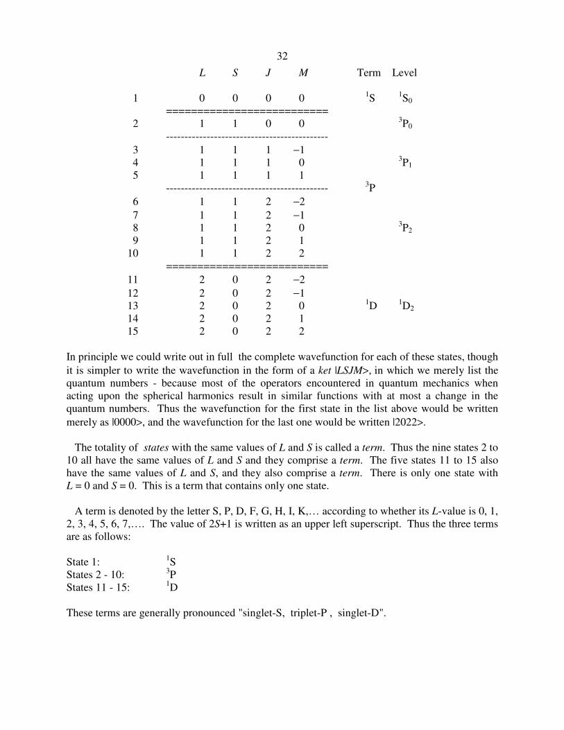
32

L S J M Term Level

1 0 0 0 0 1S 1S0 ========================== 2 1 1 0 0 3P0 -------------------------------------------- 3 1 1 1 −1 4 1 1 1 0 3P1

5 1 1 1 1 -------------------------------------------- 3P 6 1 1 2 −2 7 1 1 2 −1 8 1 1 2 0 3P2

9 1 1 2 1 10 1 1 2 2 ========================== 11 2 0 2 −2 12 2 0 2 −1 13 2 0 2 0 1D 1D2

14 2 0 2 1 15 2 0 2 2 In principle we could write out in full the complete wavefunction for each of these states, though it is simpler to write the wavefunction in the form of a ket |LSJM>, in which we merely list the quantum numbers - because most of the operators encountered in quantum mechanics when acting upon the spherical harmonics result in similar functions with at most a change in the quantum numbers. Thus the wavefunction for the first state in the list above would be written merely as |0000>, and the wavefunction for the last one would be written |2022>. The totality of states with the same values of L and S is called a term. Thus the nine states 2 to 10 all have the same values of L and S and they comprise a term. The five states 11 to 15 also have the same values of L and S, and they also comprise a term. There is only one state with L = 0 and S = 0. This is a term that contains only one state. A term is denoted by the letter S, P, D, F, G, H, I, K,… according to whether its L-value is 0, 1, 2, 3, 4, 5, 6, 7,…. The value of 2S+1 is written as an upper left superscript. Thus the three terms are as follows: State 1: 1S States 2 - 10: 3P States 11 - 15: 1D These terms are generally pronounced "singlet-S, triplet-P , singlet-D".

33

The totality of states with the same values of L, S, and J is called a level. Thus the term 3P has three levels, denoted by 3P0 ,

3P1 and 3P2 , in which the value of J is written as a bottom right subscript. Except in the presence of an external magnetic or electric field, all states belonging to a given level have the same energy, and on an energy level diagram they would appear as a single horizontal line. The number of states in a given level is 2J+1 and this is called the degeneracy d of the level. The number of levels in a term (see discussion following equation 7.13.3) is 2minL,S+ 1. This is called the multiplicity g of the term. In all of the terms discussed above arising from the configuration p2, S is less than or equal to L, and therefore the multiplicity of these terms is 2S+1, which is equal to the upper left superscript. Consider, however, the terms 3S and 5P, which occur in some other configurations. In these two cases, L < S, so the multiplicity is 2L+1. For 3S we have S = 1 and L = 0; the multiplicity is 1 and the only level in the term has J = 1. For 5P, we have S = 2 and L = 1; the multiplicity is 3 and the three levels are 5P1,2,3. Nevertheless it is customary to pronounce these terms "triplet-S, quintet-P". The statistical weight ϖ of a level or a term is the number of states in it. The statistical weight of a level is the same as its degeneracy, and is 2J+1. The statistical weight of a term is the sum of the degeneracies of its constituent levels, and is ( )( ),1212 ++ SL regardless of the relative sizes of L and S. You should verify this for each of the levels and terms in the configuration p2. The symbol ϖ, by the way, is a form of the Greek letter pi, and resembles the way in which pi is written in handwriting.

Exercise. Show that ( ) ( )( ),121212 ++=+∑+

−

SLJSL

SL

regardless of the relative sizes of L and S.

The reader might note that not all authors retain the distinction between degeneracy, multiplicity and statistical weight, or the symbols I am using to represent them. In particular, the symbol g is (regrettably) often used for the statistical weight or degeneracy of a level. It is not always clear what concept is being represented by a given symbol, and it is important in your own writing always to make it clear yourself and never to assume that your readers will understand what you intend if you not make it clear. Please also do not refer to the upper left superscript of a term as its "multiplicity". The multiplicity is 2 minL , S + 1; the upper left superscript is 2S+1. Parentage. We'll try to understand this word by means of an example, and we'll consider the neutral vanadium atom. The spectrum of vanadium is quite complex, and there are many low-lying terms. For example, among the many terms whose term values are within 3 µm-1 of the ground level are four 6D terms. These are terms with S L= =5

2 2, . The multiplicity of such a term is 5, the J-values being 1

232

52

72

92, , , , . The ground configuration of VI is KL3s

23p63d

34s2.

Here I have abbreviated the first ten electrons in the configuration with the letters KL, to indicate full K and L shells. In fact in the present discussion, I am not going to be specially interested in the first 18 electrons, and I am going to indicate the ground configuration merely by 3d

34s2. In

34

fact, none of the four 6D terms under discussion comes from this configuration. They all come from excited configurations. Specifically, in order of increasing energy, the configurations of these four 6D terms are:

3 4

3 4 4

3 4

3 4 4

4

3

4

3

d s

d s p

d p

d s p

You will notice that two of them (the second and fourth) arise from the same configuration. Let us consider how the several 6D terms arise. Consider the first of them. The configuration 3d

4 of Ti I (titanium is the element just before vanadium in the periodic table) gives rise to a great many terms (I believe it gives rise to 16 terms). In particular there is a 5D term. If you now add a 4s electron (to turn titanium into vanadium) to the 5D term of Ti I, this gives rise to two V I terms, one of which is the first of our 6D terms of interest. The 5D term of the Ti I 3d

4 configuration is called the parent of this term, and, to make this clear, the configuration of the first V I 6D term is written ( ) sd 4D3 54 In a similar manner, the configurations of the other three 6D terms of V I with their parents indicated are

( )( )

( ) psd

pd

psd

4P43

4D3

4F43

53

54

53

Many terms of V I have the same parent. Thus ( )D3 54d is parent to eight terms in the lowest 3 µm-1 of term value. The totality of terms having the same parent is called a polyad. Parity. The wavefunction that describes a particular term has the property that if it is inverted through the origin (this means, in spherical coordinates, that θ and φ are replaced by π−θ and π+φ respectively) the wavefunction is either unchanged or just changes in sign. In the former case the term is said to be of even parity; in the latter case it is of odd parity. This may sound like a rather obscure wavemechanical nicety, bit it is of sufficient importance to a working spectroscopist that he or she needs to know the parity of each term. Because of this it is usual (in fact essential) to indicate a term of odd parity by means of the upper right superscript o. Terms of odd parity, for example, might be written 3Po , 4So , etc. It is easy to know (if not to understand why) a given term has odd or even parity. If the (scalar) sum of the l-values of the

35

configuration from which a term arises is even, the parity is even; if it is odd, the parity is odd. When we earlier considered the terms arising from p2, all the terms had even parity, because the sum of the l-values of the two p electrons is 2. The reason why a working spectroscopist needs to know the parity of a term will become evident later in section 7.24 on selection rules. 7.15 Components, Lines, Multiplets, etc.

An atom can make a transition from one level to another. This may be as a result of a collision with another atom. If one (or both) of the colliding atoms moves to a higher energy level, there will be a loss of kinetic energy; the collision is inelastic. If one (or both) moves to a lower level, there will be a gain in kinetic energy; the collision is superelastic. We are concerned here, however, with transitions from one level to another involving absorption or emission of radiation (or of a photon, depending on whether you prefer to think of light as waves or as particles). If a photon is absorbed and the atom moves up to a higher energy level, the process is called photoexcitation and an absorption line is formed. If an atom falls down to a lower level it may emit a photon of appropriate frequency or wavenumber (h E Tν σ= =∆ ∆or ); this is radiative

de-excitation. It is possible for a photon of the right frequency (h Tν = ∆ ) actually to stimulate a downward transition, thus amplifying the intensity of the original photon. This process is called light amplification by stimulated emission of radiation, generally abbreviated to laser. In any case, although the transition from one level to another may well result in a change of electron configuration, the energy levels concerned are those of the atom, and it is the atom, not "the electron" that makes a transition between energy levels. This point was discussed in section 7.1. However, we have seen that a level (defined by LSJ) in fact consists of several (2J+1) states, all of which in the absence of an external magnetic or electric field, have the same energy. Evidently a line must be the totality of several transitions connecting the several states of which the two levels are composed. In the presence of a magnetic field (for example, in a sunspot) the various states within a level become separated in energy, and consequently the several components of a line become separated in wavelength. This is the Zeeman effect. These is a somewhat similar effect in the presence of an electric field, known as the Stark effect. However, stellar atmospheres are typically highly ionized plasmas and hence good electrical conductors that cannot sustain high electric potential differences, thus the Stark effect is not often met with in stellar atmosphere except on a microscopic scale when atom-atom interactions may give rise to Stark broadening of spectrum lines. Before we proceed, just a reminder. A term is defined by LS. A term comprises 2 minL , S + 1 levels, each defined by LSJ. A level comprises 2J+1 states, each defined by LSJM. Now for some more definitions. A (Zeeman) component is a transition between two states. (In most contexts, the two states will belong to different levels.) A line is the totality of components connecting two levels. (In many, but not all, contexts, the two levels will belong to different terms.) Imagine two levels, one with J = 2 (and hence five

36

states) and the other with J = 3 ( and hence seven states). In principle there are 35 ways of connecting one of the five states in one level with one of the seven states in the other. In practice, the actual number of transitions possible is rather less than this, since some of the transitions have zero probability. This will be discussed later in section 7.24 on selection rules.

A multiplet is the totality of lines connecting two terms. Imagine two terms, for example a 5P term and a 5D term. The former has three levels, the latter five. (Exercise: What are the J-values for each?) In principle there are 15 ways of connecting one of the three levels of the former with one of the five of the latter. In practice, the selection rules (see later) preclude several of these. In atomic spectroscopy, it is customary to indicate a line by writing the two levels with a dash between them, and the lower level is written first, whether the line is in emission of absorption. For example, a line might be 5

25

3P − D . If you want to specify an absorption line, you could use → rather than a dash, or ← if you want to specify an emission line. In molecular spectroscopy it is customary to write the upper state first. A multiplet in atomic spectroscopy would be written 5 5P D− . The totality of terms connecting two polyads is a supermultiplet. The totality of terms connecting two configurations is a transition array. 7.16 Return to the Hydrogen Atom.

We have until now talked about the "levels" n = 1, 2, 3… of hydrogen, and the Lyman and Balmer "lines" connecting them. This nomenclature is now suspect. In its lowest configuration the sole electron in hydrogen is in the K-shell and has n = 1. The only possible l-value is zero, and hence the lowest configuration in hydrogen is 1s. This single electron has l = 0 and s = 1/2, and hence for the atom L = 0 and S = 1/2. Thus the only term in the K-shell is 2S, and this has but a single level, 2S1/2. (We are not considering here the very small contribution made by the spin of the nucleus; this is unimportant for most contexts in optical spectroscopy, but is important - VERY important - in the microwave region.) In the L-shell, n = 2, and hence the electron can be in an s-orbital or a p-orbital. (See section 7.12 to recall the phrase "the electron is in a p-orbital".) That is, the configuration can be 2s or 2p. In either case, of course, s = 1/2, so that the two possible terms in the L-shell are 2S (with one level, 2S1/2) and 2P (with two levels, 2P1/2 and 2P3/2). I leave it up to the honour and integrity of the reader to convince him/herself that the possible configurations for n = 3 are 3s, 3p or 3d. There are three terms: 2S, 2P and 2D, 5 levels (write down the J-levels of each) and 18 states. In brief, although we have hitherto talked about the n = 1, 2, 3 levels, this is all right for n = 1, but n = 2 is three levels in two terms, and n = 3 is five levels in three terms.

37

The term values of the nine levels included in n = 1, 2 and 3 are as follows, in µm-1. I have also written out the statistical weight 2J + 1 of each level.

3 9 7492342 6

3 9 7492306 4

3 9 7492306 4

3 9 7492208 2

3 9 7492198 2

2

2

2

2

2

52

32

32

12

12

d

d

p

s

p

D

D

P

S

P

o

o

.

.

.

.

.

2 8 2259272 4

2 8 2258942 2

2 8 2258907 2

2

2

2

32

12

p

s

p

P

S

P

o

o12

.

.

.

1 0 0000000 22

12

s S .

Notice that the statistical weights of the K, L and M shells (n = 1, 2, 3) are, respectively, 2, 8 and 18 - i.e 2n

2, as explained in section 7.11. In section 7.9 (see especially immediately following equation 7.9.2), before the introduction of electron spin, we had deduced that the statistical weight of each shell was just n2; the introduction of electron spin has doubled that. So just how many transitions are there in the "line" Hα? We cannot answer that until we have familiarized ourselves with the selection rules, but I make it that Hα comprises three transition arrays, three multiplets, seven lines, and I'm not sure just how many components! We'll come back to this in section 7.24.. 7.17 How to recognize LS-coupling.

LS-coupling is in practice a good approximation in light atoms, but there are appreciable departures from LS-coupling in the heavier atoms. Generally the several lines in a multiplet in LS-coupling are fairly close together in wavelength for LS-coupling, but, as departures from LS-coupling become more pronounced, the lines in a multiplet may become more widely separated and may appear in quite different parts of the spectrum. In LS-coupling, multiplets always connect terms with the same value of S. Thus, while 3D − 3P would be "allowed" for LS-coupling, 3D − 1P would not. ∆S = 0 is a necessary condition for LS-

coupling, but is not a sufficient condition. Thus while a multiplet with ∆S ≠ 0 certainly indicates departure from LS-coupling, ∆S = 0 by no means guarantees that you have LS-coupling. In spectroscopy, the term "forbidden" generally refers to transitions that are forbidden to electric

38

dipole radiation. Transitions that are forbidden merely to LS-coupling are usually referred to as "semi-forbidden", or as "intersystem" or "intercombination" transitions. We shall have more on selection rules in section 7.24.

The energies, or term values, of the levels (each defined by LSJ) within a term are given, for LS-coupling, by a simple formula: ( ) ( ) ( )[ ].1112

1 +−+−+= SSLLJJaT 7.17.1 Here a is the spin-orbit coupling coefficient, whose value depends on the electron configuration. What is the separation in term values between two adjacent levels, say between level J and J −1? Evidently (if you apply equation 7.17.1) it is just aJ. Hence Landé's Interval

Rule, which is a good test for LS-coupling: The separation between two adjacent levels within a

term is proportional to the larger of the two J-values involved. For example, in the ( ) o32 P3S3 psKL term of Mg I (the first excited term above the ground term), the separation

between the J = 2 and J = 1 levels is 4.07 mm-1, while the separation between J = 1 and J = 0 is 2.01 mm-1. Landé's rule is approximately satisfied, showing that the term conforms closely, but not exactly, to LS-coupling. It is true that for doublet terms (and all the terms in Na I and K I for example, are doublets) this is not of much help, since there is only one interval. There are, however, other indications. For example, the value of the spin-orbit coupling coefficient can be calculated from LS-theory, though I do not do that here. Further, the relative intensities of the several lines within a multiplet (or indeed of multiplets within a polyad) can be predicted from LS-theory and compared with what is actually observed. We discuss intensities in a later chapter. The spin-orbit coupling coefficient a can be positive or negative. If it is positive, the level within a term with the largest J lies highest; such a term is called a normal term, though terms with negative a are in fact just as common as "normal" terms. If a is negative, the level with largest J lies lowest, and the term is called an inverted term. Within a shell (such as the L-shell) all the s electrons may be referred to as a subshell, and all the p electrons are another subshell. The subshell of s electrons can hold at most two electrons; the subshell of p electrons can hold at most six electrons. If the outermost subshell (i.e. the electrons responsible for the optical spectrum) is less than half full, a is positive and the terms are normal. If it is more than half full, a is negative and the terms are inverted. If the subshell is exactly half full, a is small, the term is compact and may be either normal or inverted. For example in Al I, the term 3 2 4

p P (which has three levels - write down their J-values) is normal. There are only two p electrons out of six allowed in that subshell, so the subshell is less than half full. The term 2 2 4 4

s p P of O II has four p electrons, so the subshell is more than half full, and the term is inverted. The term 2 22 3 2

s p Po of the same atom has a subshell that is exactly half full. The term happens to be normal, but the two levels are separated by only 0.15 mm-1, which is relatively quite tiny.

39

7.18 Hyperfine Structure

The levels and lines of many atoms have a hyperfine structure that is detectable only with high resolution, which may require not only interferometry but also a low temperature and low pressure source so that the intrinsic line width is small. Part of this very fine structure is due to the existence of several isotopes, and is not technically what is ordinarily meant by hyperfine structure, but is better referred to as isotope effects, which are dealt with in section 7.19. Hyperfine structure proper arises from the existence of nuclear spin, and it is this aspect that is dealt with in this section. Protons and neutrons, the constituents of an atomic nucleus, collectively known as "nucleons", have, like the electron, a spin of 1/2. That is to say, they possess an angular momentum

( ) ,31 21

21

21

hh =+ oriented such that the component in some direction can have only one of

the two values .21h± Consequently a nucleus with an even number of nucleons must have an

integral spin (which might be zero) while a nucleus with an odd number of nucleons must have an integral-plus-half spin, which cannot be zero. The spin quantum number of a nucleus is

denoted by the symbol I. The magnitude of the nuclear angular momentum is ( ) .1 h+II It should be noted that different isotopes of a given element in general have different nuclear spins and consequently different hyperfine structure. Whether the electrons in an atom are coupled by LS or jj or intermediate coupling, the coupling between the electrons is much stronger than the weak coupling between electrons and nucleus. Thus, in considering the coupling between the electrons and the nucleus, J can usually be regarded as a "good quantum number". To determine the total angular momentum of an atom, we have to add (vectorially, and by the rules of quantum mechanics) the nuclear angular momentum I to the electronic angular momentum J. This forms the total angular momentum of the atom, including nuclear spin, denoted by the symbol F: F = J + I. 7.18.1 This equation is very similar to equation 7.13.3, except that, in equation 7.13.3, although S can be either integral or integral-plus-one-half, L is integral; whereas, in equation 7.18.1 both J and I have the possibility of being either integral or integral-plus-one-half. In any case, there are 2minI , J + 1 values of F, going from J I J I− +to . If J + I is integral, all values of F are integral; and if J + I is integral-plus-one-half, so are all values of F. The magnitude of F is

( ) .1 h+FF The nature of the interaction between J and I is the same as that between L and S in LS-coupling, and consequently the spacing of the term values of the hyperfine levels is similar to that described by equation 7.17.1 for the spacing of the levels within a term for LS-coupling namely: ( ) ( ) ( )[ ],1112

1 +−+−+= IIJJFFbT 7.18.2

40

except that b<<a. Landé's interval rule is obeyed; that is to say, the separation of two hyperfine levels within a level is proportional to the larger of the two F-values involved.. There are similar selection rules for transitions between the hyperfine levels of one level and those of another, namely ( ),forbidden001,0and ↔±=∆∆ JF and (naturally!) ∆I = 0. Calculating the spacings and intensities in the hyperfine structure of a line is precisely like calculating the spacings and intensities of the lines within a multiplet in LS-coupling. For nuclei with zero spin, the quantum number M was associated with the vector J, which was oriented such that its z-component was hM , where M could have any of the 2J+1 values from −J to +J. (We are here describing the situation in the quasi-mechanical descriptive vector model, rather than in terms of the possible eigenvalues of the quantum-mechanical operators, which supplies the real reason for the restricted values of the quantum numbers.) With nuclear spin, however, the quantum number M is associated with the vector F, which is oriented such that its z-component is hM , where M can have any of the 2F+1 values from −F to +F, these values being integral or integral-plus-one-half according to whether F is integral or integral-plus-one-half. Thus each level is split into 2minJ , I + 1 hyperfine levels, and each hyperfine level is (2F+1)-fold degenerate. Thus the statistical weight of a level is ( ) ).12(12 ++ JI (For a derivation of this, recall the Exercise in Section 7.14 concerning the statistical weight of a term in LS-coupling.) If the nuclear spin is zero, the statistical weight of a level is the same as its degeneracy, namely just 2J+1. For nonzero nuclear spin, the correct expression for the statistical weight is (2I+1)(2J+1). Nevertheless, the statistical weight is often treated as though it were merely 2J+1, and indeed there are many contexts in which this can be safely done. We shall return to this in Chapter 9 when discussing the Boltzmann and Saha equations. Hyperfine structure of spectrum lines is not often evident in the visible spectrum of stars. Generally the resolution is too poor and the lines are so broadened by high temperature as to mask any hyperfine structure. However, the nuclear spin of, for example, the 51V (vanadium) atom is I = 7/2, and the hyperfine structure of the lines, even if not fully resolved, is sufficient to make the lines noticeably broad. In the radio region, the most famous line of all is the 21-cm line of atomic hydrogen, and this involves hyperfine structure. The ground term of H I is 1s 2S, which consists of the single level 2S1/2. This level has J = 1

2 . The nuclear spin (spin of a proton) is I = 1

2 , so the level is split into two hyperfine levels with F = 0 and 1. The 21-cm line is the transition between these two hyperfine levels. The transition is forbidden to electric dipole radiation (there is no parity change) and so it involves magnetic dipole radiation. It is therefore intrinsically a very weak line, but there is an awful lot of space out there with an awful lot of hydrogen in it. 7.19 Isotope effects.

The existence of different isotopes of an element gives rise to what could be called hyperfine structure, except that we are restricting the use of the term hyperfine structure to the splitting caused by nuclear spin. There are two quite different isotope effects, which I refer to as the mass

effect and the volume effect.

41

The effect of different isotopic masses is to displace the centre of mass between nucleus and electrons a small amount. In the hydrogen atom, for example, the term values (neglecting fine structure and referring to the Bohr model) are given by equation 7.4.9, in which the expression

for the Rydberg constant includes the reduced mass µ =+

Mm

M m of the electron. It becomes a

simple matter to calculate the energy levels and Balmer wavelengths of D, He+, Li++, etc., merely by exchanging the reduced mass in H by the reduced mass in the other species. I commend this exercise to the reader. For example, by how much does the wavelength of Hα differ in the spectra of ordinary hydrogen and deuterium? For more complex atoms, the calculation of the isotope shift is more difficult, but the basic reason for the shift is the same. It might well be thought that isotope shifts would be greatest for very light atoms, but would be negligible for heavier atoms, because the displacement of the position of the centres of mass in different isotopes of a heavy atoms such as, for example, iron, would be negligible. This is indeed the case for the mass isotope effect. It comes as something of a surprise, therefore, to learn that there are significant isotope shifts between isotopes of quite massive isotopes, such as lead, cadmium, gold, mercury, promethium and osmium, and that such shifts have even been observed in stellar spectra. The shift is a result of the relatively large volumes of these nuclei. There is no need to go into the detailed theory of the volume effect here, though it is at least useful to know of its existence and, to some extent, its cause. An allowed electric dipole line always involves a transition between two levels belonging to different configurations, and the volume effect is most marked for those transitions in which the two configurations have different numbers of s-electrons. These are electrons with zero orbital spin angular momentum, and, in the Bohr-Sommerfeld atomic model (mentioned briefly in section 7.4), these orbits would be ellipses that have degenerated into straight lines through the nucleus. In other words, we can understand that the volume effect is related to the penetration of the nuclei by s-electrons, and we can see why the effect is most marked in the largest nuclei. 7.20 Orbiting and Spinning Charges. In the next section, section 7.21, we are going to look at the Zeeman effect, which is the symmetric splitting of spectrum lines in a magnetic field. Before we get to that, however, it will be useful to review some elementary principles of classical mechanics and electromagnetism in relation to orbiting and spinning electric charges. In particular, an orbiting or a spinning electric charge has angular momentum and also a magnetic moment. In this section we shall calculate both of these quantities for an orbiting charge and for a spinning charge. In particular we shall calculate for each the ratio of the magnetic moment to the angular momentum for each. This quantity should be called the magnetogyric ratio, though for some reason some people refer to it, entirely illogically, as the “gyromagnetic” ratio. We shall start by considering a point electric charge of mass m and charge e moving with speed v in a circle of radius a. It is elementary classical mechanics that its angular momentum is mva. This may be seen either by thinking of angular momentum as synonymous with moment of

momentum (in which case the moment of momentum is mv times a) or thinking of angular

42

momentum as Iω (in which case it is ma2 times v / a). The dimensions of angular momentum are

ML2T-1, and the SI units are conveniently expressed as J s (joule seconds). You should check that the dimensions of J s are correct. Before calculating the magnetic moment, it is worth while to consider what is meant by magnetic moment. This is because there are several different ways in which magnetic moment could be defined (I can think of twelve plausible definitions!) and it by no means clear what different authors think that they mean by the term. I shall use the following concept (which is standard SI). If a magnet is placed in an external magnetic field B (of which the SI unit is tesla), the magnet will in general experience a torque. (I say "in general" because if the magnetic moment is parallel or antiparallel to the field, there will be no torque.) The magnitude of the torque depends on the orientation of the magnet with respect to the torque. There are two particular directions (opposite to each other - i.e. differing by 180o) in which the torque is a maximum. Definition: The magnetic dipole moment is the maximum torque experienced in unit magnetic

field B. It is a vector quantity, and I propose to use the symbol µ µ µ µ for it, or µ for its magnitude, unless contexts arise in which µ might be confused with something else (such as permeability, for example). I shall warn if I need to use an alternative symbol. With that definition, the expression for the torque ττττ on a magnet of moment µµµµ in a external field B is ττττ = µµµµ × B 7.20.1 This equation alone will not define µµµµ uniquely, for (if you have experienced solutions of vector equations before) the equation cannot be solved uniquely for µµµµ. However, in concert with the definition given in the italicized sentence above, the magnetic moment is defined uniquely and without ambiguity. The SI unit is N m T-1. (J T-1 would also do in principle, except that joule does not suggest the concept of torque as well as N m does.) An example is usually given in introductory electricity courses for the torque on a plane, current-carrying coil, in which it is shown that the magnetic moment in that case is equal to the current times the area of the coil (times the number of turns if there are more than one). Thus equivalent and fully acceptable SI units are A m2. The dimensions of magnetic moment are IL2. (It will be noted that magnetic moment is often quoted in other units such as T m3 or G cm3. If not actually wrong, these must describe dimensionally different definitions of what is meant by magnetic moment. T m3, for example, is not dimensionally the same as N m T-1. I do not pursue this aspect here; I have given the standard SI treatment.) With that introduction, we can now move to calculate the magnetic moment of a point electric charge e moving with speed v in a circle of radius a. The effective current is the charge divided by the period of the orbit, which is e ÷ (2πa / v ) = ev / (2πa). The area of the circle is πa

2, so the magnetic moment is eav / 2.

The ratio of the magnetic moment to the angular momentum, i.e. the magnetogyric ratio, is e

m2.

The SI unit is C kg-1. For an electron moving in a circle (of whatever radius and at whatever speed) its magnitude is 8.794 × 1010 C kg-1.

43

What about a spinning sphere of finite radius? Well, if the charge and the mass are both uniformly distributed throughout the sphere, or if they are not uniformly distributed but charge and mass are equally distributed throughout the sphere, then the magnetogyric ratio is again just

e

m2, because every little element of the spinning sphere can be considered to be a point charge

moving in a circle. But what if the charge and mass densities are distributed differently? For example, if the sphere were a charged metal sphere, in which the mass is distributed uniformly through the sphere, but the charge is confined to the surface? In this case you would expect the magnetogyric ratio to be

a good deal greater than 12

. .e

m You will probably find it easy to calculate the angular

momentum of a uniform sphere of mass m and radius a spinning at angular speed ω. It will be slightly more difficult, but a very good exercise, to work out the magnetic moment, assuming that

all the charge is on the surface. You should find that the magnetogyric ratio is 56

. e

m, which, as

expected, is a good deal larger than 12

. .e

m From this it might be anticipated that, if we could

somehow measure (perhaps from the Zeeman effect) the magnetogyric ratio of an electron (which, indeed, we can, and with quite extraordinary precision) we can get some information about how mass and charge are distributed throughout the electron. In fact it turns out that the magnetogyric ratio of a spinning electron is very close to e/m. This suggests not only that the charge is distributed near to the surface but that the mass is concentrated near to the centre. Is this true? It is true that we can measure the magnetogyric ratio spectroscopically, and it is true that it turns out to be very close to ./ me Whether deducing from this that an electron is a sphere in which the charge is held near the surface and the mass is centrally concentrated is a bit more problematical. It is not necessarily "wrong", but it may not be a very useful model to describe other properties of the electron beyond its magnetogyric ratio. Particle physicists generally regard an electron as a "lepton" without any discernible internal structure. Perhaps physics cannot say what an electron (or anything else) really "is"; we can describe its observable properties and use whatever models appear best to describe these and to predict its behaviour. I move now to the question of what is the potential energy of a magnet of moment µµµµ when it is situated in a magnetic field B. When the angle between µµµµ and B is θ, there is a torque on the magnet of magnitude µB sin θ (see equation 7.20.1)). The work needed to increase θ by dθ is µ θ θB dsin , and the work needed to go from θ1 to θ2 is therefore ( )21 coscos θ−θµB , which is the difference in potential energy between the two positions. We may choose the zero level for potential energy where we will. If, for example, we choose the potential energy to be zero when µµµµ and B are parallel, the potential energy at angle θ is ( ).cos1 θ−µB If, on the other hand, we choose the potential energy to be zero when µµµµ and B are at right angles to each other (as is very often done), the potential energy at angle θ is −µ θB cos , or −µµµµ • ΒΒΒΒ. With this convention, the potential energy is −µB, 0 or +µB for µµµµ and B parallel, perpendicular or antiparallel.

44

One last topic before proceeding to the Zeeman effect. Those who have studied classical mechanics will appreciate that if a spinning body, of angular momentum L is subjected to an external torque ττττ, it will precess with an angular speed ΩΩΩΩ, and the three vectors are related by ττττ = ΩΩΩΩ × L . 7.20.2 Again, those familiar with vector equations will note that this equation cannot be solved uniquely for ΩΩΩΩ, because we don't know the angle between τ τ τ τ and L . If, however, we are dealing with a nonvertical top spinning on a table, the torque is at right angles to the angular momentum vector and the rate of precession is mgl / L, where l is the distance between the bottom of the top (sorry for the choice of words) and the centre of mass. (Those who are very familiar with the theory of the top, will recognize that we are here referring to the rate of true or pseudo regular precession, after nutational motion has been damped out - but there is no need for such niceties here.)

Now consider a spinning magnet whose magnetic moment is µ µ µ µ and whose angular momentum is L. Suppose it is placed in a magnetic field B. It now experiences a torque ττττ = µµµµ × B. The result of this is that, regardless of the angle between L and B, L will precess around B at an angular speed µB/L. That is to say, at an angular speed equal to B times the magnetogyric ratio. In the case of a particle of charge e and mass m moving in a circle the angular speed of

precession is eB

m2. This is called the Larmor angular speed, and

eB

m4π is the Larmor frequency.

If e, B and m are expressed in C, T and kg respectively, the Larmor frequency will be in Hz. 7.21 Zeeman effect When a hot gas which is emitting or absorbing spectrum lines is placed in a magnetic field, the lines become split into several components. This is known as the Zeeman effect, discovered in 1896 by the Dutch spectroscopist P. Zeeman. If we start by thinking of an atom with zero nuclear spin, it will be recalled that every energy level except those with J = 0 is degenerate. That is, there are 2J + 1 wavefunctions, or eigenstates, or just states, each described by a quantum number M, which goes from −J to +J, and each of these states has exactly the same energy. When the atom is placed in an external magnetic field, this degeneracy is removed, and each state has a slightly different energy. This happens to both levels involved in the formation of a line (unless one of the levels has J = 0), with the result that the line that joins the two levels is split up into a number of components. It will be recalled that a line joins two levels. In a similar manner a (Zeeman) component joins two states. Just as a multiplet is the totality of lines joining two terms, so a line is the totality of components joining two levels. In the absence of a magnetic field, all the states within a level have the same energy, and all the components that make up a line have the same wavelength. A term is described by LS. Its multiplicity is 2 minL , S +1 and its statistical weight is ( )( )1212 ++ SL . A level is described by LSJ. Its degeneracy and statistical weight are 2J + 1. A state is described by LSJM. It is not degenerate; its statistical weight is 1.

45

In sections 9 ,10, and 11 of this chapter, I went to some trouble to persuade you that an electron is not a hard, spinning sphere that moves in a circular orbit around a nucleus. Rather I described electrons in terms of wavefunctions that describe the probability amplitude, and quantum numbers were eigenvalues of certain operators and were restricted to certain values as a result of boundary conditions. What model we use to describe the behaviour of atoms depends on our purpose, and, if our purpose was to obtain expertise in the intricacies of quantum mechanical calculations, we would have to become heavily involved in the algebra of kets, operators and eigenfunctions. Our present purpose, however, is to become acquainted in a rather descriptive way with spectroscopy, and in describing Zeeman phenomena without the intention of performing quantum mechanical calculations. It will be convenient to revert to a model of an electron, if not as a hard, spinning, orbiting particle, at least as an entity that possesses the attributes of orbital and spin angular momentum and consequently also of magnetic moment.

In particular, we recall that an orbiting electron has an orbital angular momentum ( )h1+ll ,

where ( )π= 2/hh has the value 1.055 × 10−34 J s. Now, if we take the magnetogyric ratio of an

orbiting electron to be ( )me 2/ , the magnetic moment of an orbiting electron is ( ) .2

.1m

ell

h+

(Those who object to this simple treatment - and there are some rather obvious objections - will have no alternative but to do a proper quantum mechanical derivation, though the result is the

same.) In any case, the quantity m

e

2

h, a unit of magnetic moment, is called the Bohr magneton,

and its value is 9.274 × 10−24 N m T−1 or A m2. I shall use the symbol µB to indicate the Bohr

magneton. Thus the orbital angular momentum of an electron is ( )h1+ll and its magnetic

moment is ( ) Bll µ+1 The magnetogyric ratio of an orbiting electron (not taking into account the contribution to angular momentum and magnetic moment from its spin) is

( ) 1010794.82// ×==µ meB h C kg−1, or, if we agree to express angular momentum in units of h and magnetic moment in units of Bohr magnetons, the magnetogyric ratio of an orbiting electron (still taking no account of the contributions of spin) is 1. The spin angular momentum

of an electron is ( ) ,1 h+ss where s =1/2, and its magnetic moment is (very close to)

( ) ,12 Bss µ+ so that its magnetogyric ratio is just e/m, or, in units of µ and h , it is 2. (The

exact value of the magnetogyric ratio, in units of h/Bµ , is a little more than 2, and is one of the most precisely-known of the fundamental physical constants. Its value in the year 2000 is given as 2.002 319 304 374.) In discussion of the Zeeman effect, we shall need to know the magnetogyric ratio of the atom in a given level, since this determines the way in which the levels are split in a magnetic field. The ratio of the magnetic moment in units of µB to the angular momentum in units of h is known as the Landé splitting factor, and is generally denoted by the symbol g. It is the magnetogyric ratio in units of ( ),2/ me or 8.794 × 1010 C kg-1. The magnetogyric ratio, or Landé splitting factor, of an atom in a given level depends on the angle between the vectors L and S and hence on their resultant J, and , though I do not do it here, it is not difficult to show that, in the case of LS-coupling, the Landé splitting factor has the value

46

( ) ( ) ( )

( ).

12111

1+

+−++++=

JJ

LLSSJJg 7.21.1

(This formula is calculated using the approximate value 2 for the magnetogyric ratio of the electron rather than the more accurate 2.00232. More accurately, it should be written

( ) ( ) ( )

( ).

12111

00232.11+

+−++++=

JJ

LLSSJJg 7.21.2

Formulas for the g-factor for other coupling schemes are available, but I do not give them here, since in practice the coupling between electron angular momenta in complex atoms is usually intermediate between idealized extremes, and the calculation has to be done numerically. In many of the lightest atoms, however, pure LS-coupling is a good approximation. The g-value can be found experimentally from observations of the Zeeman effect, and, in addition to Landé's interval rule mentioned earlier, this affords another good indication of how close a level is to LS-coupling. Problem. The 5

15

0P Do− line of Fe I at 617.33 nm is often used to investigate magnetic fields in sunspots. The strongest line of the multiplet that includes this line is 5

35

4P Do− . Calculate the g-factor for each of the four levels mentioned.

A small point to be made is as follows. From what we have said, the magnetic moment of an atom (excluding nuclear spin, if any) is of magnitude ( ).1+µ=µ JJg B (This follows from the definition of g, which is the ratio of the magnetic moment in units of the Bohr magneton - i.e. µ/µB - to the angular momentum in units of h .) In vector form this must be written µµµµ = −gµBJ, where J is a dimensionless vector of magnitude ( )1+JJ and the minus sign arises because of the negative electron charge, the magnetic moment and angular momentum vectors being oppositely directed. When the Zeeman effect was first investigated, lines were observed to be split into just three components, and this was referred to as the normal Zeeman effect. Later, more complex patterns were observed, and this was referred to as the anomalous Zeeman effect. As we now understand it, the so-called "normal" Zeeman effect is merely the Zeeman effect observed on lines joining levels with spin S = 0, which have a simpler Zeeman pattern than other lines. In addition to the Stern-Gerlach experiment, it was the study of "anomalous" Zeeman splitting that gave rise to the discovery of electron spin. We are now in a position to start looking at how energy levels are split in the presence of a magnetic field. Let us consider, for example, a 1P1 level (L, S, J = 1, 0, 1). The Landé factor is 1. (Note that for any level in which S = 0 and therefore in which J and L are necessarily equal, equation 7.21.1 (or 7.21.2) shows that g = 1.)

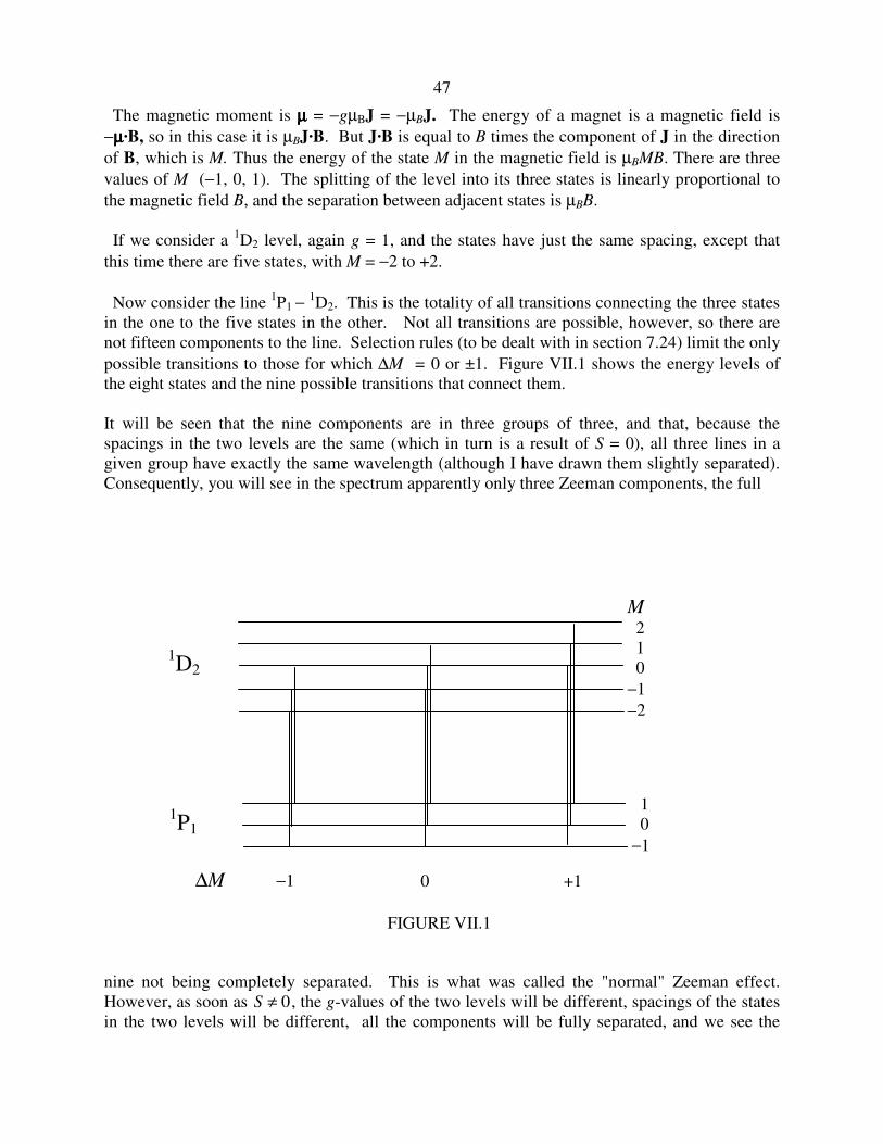
47

The magnetic moment is µµµµ = −gµBJ = −µBJ. The energy of a magnet is a magnetic field is −µµµµ·B, so in this case it is µBJ·B. But J·B is equal to B times the component of J in the direction of B, which is M. Thus the energy of the state M in the magnetic field is µBMB. There are three values of M (−1, 0, 1). The splitting of the level into its three states is linearly proportional to the magnetic field B, and the separation between adjacent states is µBB. If we consider a 1D2 level, again g = 1, and the states have just the same spacing, except that this time there are five states, with M = −2 to +2. Now consider the line 1P1 − 1D2. This is the totality of all transitions connecting the three states in the one to the five states in the other. Not all transitions are possible, however, so there are not fifteen components to the line. Selection rules (to be dealt with in section 7.24) limit the only possible transitions to those for which ∆M = 0 or ±1. Figure VII.1 shows the energy levels of the eight states and the nine possible transitions that connect them. It will be seen that the nine components are in three groups of three, and that, because the spacings in the two levels are the same (which in turn is a result of S = 0), all three lines in a given group have exactly the same wavelength (although I have drawn them slightly separated). Consequently, you will see in the spectrum apparently only three Zeeman components, the full nine not being completely separated. This is what was called the "normal" Zeeman effect. However, as soon as S ≠ 0 , the g-values of the two levels will be different, spacings of the states in the two levels will be different, all the components will be fully separated, and we see the

1D2

1P1

M 2 1 0 −1 −2

1 0 −1

∆M −1 0 +1

FIGURE VII.1

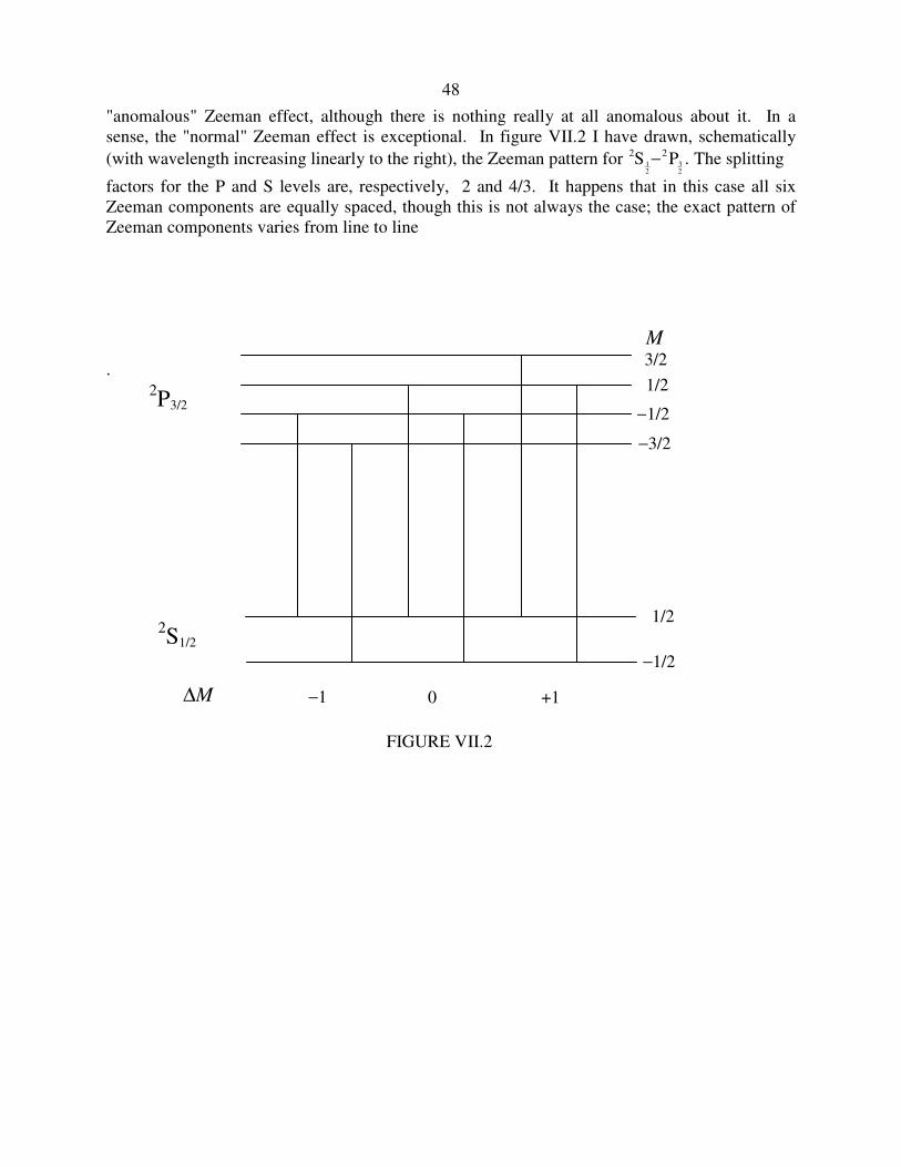
48

"anomalous" Zeeman effect, although there is nothing really at all anomalous about it. In a sense, the "normal" Zeeman effect is exceptional. In figure VII.2 I have drawn, schematically (with wavelength increasing linearly to the right), the Zeeman pattern for 2 2

32

S P12− . The splitting

factors for the P and S levels are, respectively, 2 and 4/3. It happens that in this case all six Zeeman components are equally spaced, though this is not always the case; the exact pattern of Zeeman components varies from line to line .

2P3/2

2S1/2

M 3/2 1/2

−1/2

−3/2

−1/2

1/2

∆M −1 0 +1

FIGURE VII.2

49

7.22 Paschen-Back Effect

The description I have given so far of the way in which a level is split up and the states are separated in a magnetic field is good for relatively weak magnetic fields, but begins to break down for strong fields. What do I mean by "weak" and "strong"? The type of splitting I have described starts to break down when the energy separation of the states of a level becomes comparable to the separation of the levels within a multiplet. Stated otherwise, it breaks down when the strength of the coupling between J and B becomes comparable to the strength of the coupling between L and S. At that stage, the coupling between L and S breaks down, and J ceases to be a "good quantum number". L and S become separately coupled to, and precess separately around, B. The components of L and S in the direction of B, in units of h , are ML and MS, with possible values from −L to +L and −S to +S. respectively. The interaction energies between L and B and between S and B, are, respectively, µBMLB and 2µBMSB, and there will also be a relatively small remanent spin-orbit interaction between L and S, represented by AMLMS, so the total interaction energy, which determines the splitting of the level into separate states, is ( ) .2 SLBSL MAMBMM +µ+ This gives rise to a quite different pattern of splitting of the levels into their constituent states, and consequently a quite different pattern of the splitting of a line into its components. This is the Paschen-Back effect. The Landé splitting factor can then no longer be defined as the ratio of the magnetic moment in Bohr magnetons to the angular momentum in units of h . L and S are no longer coupled to each other, and J is no longer a good quantum number. Rather, the g-factor is the ratio of the sum of the components of the orbital and spin magnetic moments in the direction of B to the sum of the components of the orbital and spin angular momenta in that direction. That is

gM M

M M

L S

L S

=+

+

2 . 7.22.1

Problem. The first excited term of Mg I is a 3Po term. The separation in term values between the levels J = 0 and J = 1 is 20 cm-1 and between J = 1 and J = 2 is 40 cm-1, so that the multiplet evidently conforms to Landé's interval rule and hence to LS-coupling. How large a magnetic field, in tesla, would be necessary so that splitting of the states within the 3 oP1 level is 20 cm-1? (I make it about 29 T, which is a very strong field.) Problem. On a sheet of graph paper, draw the three levels of a 3P multiplet. Choose a scale so that the spin-orbit coupling coefficient (equation 7.17.1) a = one inch, so that the energy levels of the three levels of the term are at −2, −1 and +1 inches. The J = 0 level has only one state, and the g-values for the other two levels are each 1.5. Now apply a weak magnetic field, thus separating the states, and to the right of your zero-field energy level diagram of the three levels draw the energy levels for the nine states, such that the separation between adjacent states is one tenth of an inch. The J = 0 level, of course, is not split. The other two levels are split into three and five states. Mark the value of MJ against each state. (We have previously used the symbol M, but in the present context, let's call it MJ so as to be able to distinguish it from ML and MS.) You now have the Zeeman effect. Now apply a strong field. Since S and L are each 1, the projections of each can be −1, 0, +1, so there are nine combinations of ML and MS. For each of

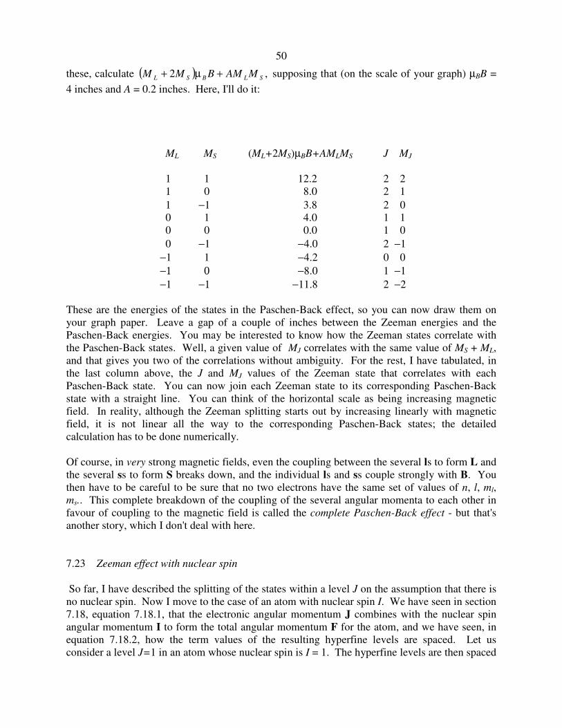
50

these, calculate ( ) ,2 SLBSL MMABMM +µ+ supposing that (on the scale of your graph) µBB = 4 inches and A = 0.2 inches. Here, I'll do it:

ML MS (ML+2MS)µBB+AMLMS J MJ

1 1 12.2 2 2 1 0 8.0 2 1 1 −1 3.8 2 0 0 1 4.0 1 1 0 0 0.0 1 0 0 −1 −4.0 2 −1 −1 1 −4.2 0 0 −1 0 −8.0 1 −1 −1 −1 −11.8 2 −2 These are the energies of the states in the Paschen-Back effect, so you can now draw them on your graph paper. Leave a gap of a couple of inches between the Zeeman energies and the Paschen-Back energies. You may be interested to know how the Zeeman states correlate with the Paschen-Back states. Well, a given value of MJ correlates with the same value of MS + ML, and that gives you two of the correlations without ambiguity. For the rest, I have tabulated, in the last column above, the J and MJ values of the Zeeman state that correlates with each Paschen-Back state. You can now join each Zeeman state to its corresponding Paschen-Back state with a straight line. You can think of the horizontal scale as being increasing magnetic field. In reality, although the Zeeman splitting starts out by increasing linearly with magnetic field, it is not linear all the way to the corresponding Paschen-Back states; the detailed calculation has to be done numerically. Of course, in very strong magnetic fields, even the coupling between the several ls to form L and the several ss to form S breaks down, and the individual ls and ss couple strongly with B. You then have to be careful to be sure that no two electrons have the same set of values of n, l, ml, ms.. This complete breakdown of the coupling of the several angular momenta to each other in favour of coupling to the magnetic field is called the complete Paschen-Back effect - but that's another story, which I don't deal with here.

7.23 Zeeman effect with nuclear spin

So far, I have described the splitting of the states within a level J on the assumption that there is no nuclear spin. Now I move to the case of an atom with nuclear spin I. We have seen in section 7.18, equation 7.18.1, that the electronic angular momentum J combines with the nuclear spin angular momentum I to form the total angular momentum F for the atom, and we have seen, in equation 7.18.2, how the term values of the resulting hyperfine levels are spaced. Let us consider a level J=1 in an atom whose nuclear spin is I = 1. The hyperfine levels are then spaced

51

in exactly the same manner as the levels are placed in a 3P term (L = 1, S = 1). Draw the three hyperfine levels on your graph paper, with the F = 0, 1, 2 hyperfine levels at −0.2, −0.1 and +0.1 inches respectively. Now, if you apply a very small magnetic field, each hyperfine level will be split up into 2F+1 equally-spaced states. But you must now bear in mind that the coupling between J and I is exceedingly weak (i.e. the spacings between the hyperfine levels is exceedingly small), so this Zeeman effect will obtain for only very tiny magnetic fields indeed. As soon as the magnetic field is at all appreciable, J and I uncouple from each other and they then couple independently with B to form a Paschen-Back effect. Does this make life unbearably complicated? As it turns out - not at all! The separation of the states is given by exactly the same sort of expression as for the Paschen-Back effect earlier described, namely ( ) IJBIIJ MAMBMgM +µ+ , except that the nuclear g-factor is not 2 as in the case of the electron, but is of order 10-3. This makes a world of difference to the way the states are separated. Let us calculate the term values, as we did before with the Paschen-Back effect, and we'll use the same field strength as before so that µBB is represented by 4 inches, but this time, purely for illustrative purposes, we'll put gI = 0.002 and A = 0.0002 inches. The result of the calculation (which you should carry out yourself - it is very quick with a programmable calculator, though tedious without) is as follows: MI MJ ( ) IJBIIJ MAMBMgM +µ+ F MF

1 1 4.01 2 2 1 0 0.01 2 1 1 −1 −3.99 2 0 0 1 4.00 1 1 0 0 0.00 1 0 0 −1 −4.00 2 −1 −1 1 3.99 0 0 −1 0 −0.01 1 −1 −1 −1 −4.01 2 −2 Now please do draw these out on your graph paper. You will find that the states are spaced in three widely-separated groups of three, with three closely-separated states in each group. You will not appreciate exactly what is happening unless you actually draw it out. But , if you do, you will see that, if your resolution is such that you cannot resolve the hyperfine structure in the zero-field situation, and you are unaware of or do not care about the nuclear spin, and you think that you have but a single level with J = 1, when you apply a magnetic field what happens is this: you will find that this level is apparently split into three "states" (which you cannot resolve into their several genuine states), and it will appear that you have a perfectly ordinary Zeeman effect in which the nuclear spin plays no role at all. Only with high-resolution, cold-source, interferometric resolution will you see the hyperfine structure of each component into hyperfine components.

52

7.24 Selection rules It will be recalled that a multiplet is the totality of transitions between two terms. For example, 3P − 3Do is the multiplet connecting the two terms 3P and 3Do. Each term has three levels, and therefore there are nine ways of connecting the levels of one term with the other, each transition resulting in a line. But in fact only six of these transitions are "allowed" or "permitted", the remaining three being "forbidden". This is because of certain "selection rules", or restrictions in the way some of the quantum number can change. Likewise there are restrictions on the number of multiplets that can connect the terms of two polyads, or on the number of Zeeman components that can connect the states of two levels. In all of these situations there are selection rules that restrict certain quantum numbers from changing by other than certain amounts. In this section we shall try to understand in a qualitative way how such selection rules arise. We shall list the various selection rules, and see how this will affect the number of lines in a multiplet, or the number of components in a line. Everyone knows that when an electric dipole oscillates it radiates an electromagnetic wave. Likewise, if a dipole, rather than periodically oscillating, suddenly undergoes a change in its electric dipole moment − for example, if the distance between two opposite electric charges suddenly changes − a pulse of electromagnetic radiation will be radiated. While the radiation from a single atom will be radiated like that of a dipole, in a gas with enormous numbers of atoms oriented in completely random directions, the radiation will appear isotropic. One reasonable way of explaining how an atom radiates a pulse (a quantum) of electromagnetic radiation when it changes from one state to another is that its dipole moment changes, and the energy radiated is related to the change in its dipole moment. Indeed in quantum mechanics, the amount of energy radiated when an atom changes from one state to another is determined by the square of a quantity known as the transition moment: .* τψψ∫ dif µµµµ

Here dτ is the usual volume element, and ψI is the wavefunction of the initial state. µµµµ is the dipole moment operator, which depends on the positions of all the electrons in the atom. ψ*

f is the conjugate of the wavefunction of the final state. Those who have lots of practice in performing such calculations are experienced enough to know that the effect of the dipole moment operator is merely to produce a similar wavefunction with perhaps some changes in the quantum numbers. Therefore, in order to save writing out the complete expression for the wavefunction in full, they merely list the quantum numbers of the initial wavefunction in a ket, and of the conjugate of the final function in a bra, thus: < >L S J M LSJM' ' ' ' | | .µµµµ Again, those who do such calculations daily for a living soon recognize, from the very symmetries of the wavefunctions (group theory) and without having to worry greatly about the details of the functions, that this transition moment is zero unless there are certain relations between the initial and final quantum numbers. It is those transitions that result in a nonzero

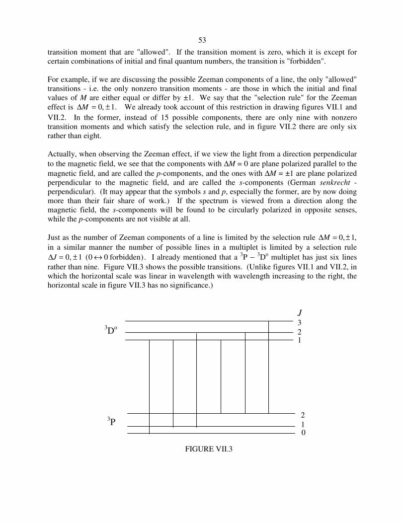
53

transition moment that are "allowed". If the transition moment is zero, which it is except for certain combinations of initial and final quantum numbers, the transition is "forbidden". For example, if we are discussing the possible Zeeman components of a line, the only "allowed" transitions - i.e. the only nonzero transition moments - are those in which the initial and final values of M are either equal or differ by ±1. We say that the "selection rule" for the Zeeman effect is .1,0 ±=∆M We already took account of this restriction in drawing figures VII.1 and VII.2. In the former, instead of 15 possible components, there are only nine with nonzero transition moments and which satisfy the selection rule, and in figure VII.2 there are only six rather than eight. Actually, when observing the Zeeman effect, if we view the light from a direction perpendicular to the magnetic field, we see that the components with ∆M = 0 are plane polarized parallel to the magnetic field, and are called the p-components, and the ones with ∆M = ±1 are plane polarized perpendicular to the magnetic field, and are called the s-components (German senkrecht - perpendicular). (It may appear that the symbols s and p, especially the former, are by now doing more than their fair share of work.) If the spectrum is viewed from a direction along the magnetic field, the s-components will be found to be circularly polarized in opposite senses, while the p-components are not visible at all. Just as the number of Zeeman components of a line is limited by the selection rule ∆M = ±0 1, , in a similar manner the number of possible lines in a multiplet is limited by a selection rule ∆J = ± ↔0 1 0 0, ( )forbidden . I already mentioned that a 3P − 3Do multiplet has just six lines rather than nine. Figure VII.3 shows the possible transitions. (Unlike figures VII.1 and VII.2, in which the horizontal scale was linear in wavelength with wavelength increasing to the right, the horizontal scale in figure VII.3 has no significance.)

3Do

3P

J 3 2

2 1 0

FIGURE VII.3

1

54

It may be that a line, or a component, is forbidden to dipole radiation and that, if µµµµ is the electric dipole moment operator, the transition moment is zero. However, if we substitute for the dipole moment operator the operator for electric quadrupole or magnetic dipole moment, the transition moment is not zero. In that case a transition that is forbidden to electric dipole (E1) radiation may be permitted to electric quadrupole (E2) or magnetic dipole (M1) radiation. E2 and M1 transitions are very weak and are rarely observed under laboratory conditions (though they occur in astronomical sources for reasons that will be explained later). Therefore lines that are forbidden to electric dipole radiation are generally referred to merely as "forbidden" lines - even though they are not actually forbidden to E2 or M1 radiation. The carrier (atom) for a forbidden line is often written in brackets. For example, there is an E2 line in the spectrum of the aurora at 557.7 nm arising from the neutral oxygen atom, so the line is said to be a line of [O I]. Some multiplets are forbidden to electric dipole radiation only if the terms concerned conform strictly to LS-coupling, but may be allowed for electric dipole radiation if there are departures from LS-coupling. Such transitions are "semi-forbidden", and the carrier is sometimes written between a bracket and a parenthesis. Thus there is a semi-forbidden line at 345.3 nm due to [Al I). For LS-coupling, electric dipole radiation is allowed only if ∆S = 0. That is to say, transitions are allowed between two triplet terms, or between two singlet terms, but not between a triplet or a singlet. (In this connection I am referring to a 3S term as a "triplet" term, even though it has just one level.) Not everyone uses this bracket-parenthesis convention. In the neutral helium atom, there are singlet terms and triplet terms. LS-coupling is the norm, and, because of this, there are no transitions between any of the singlet terms and a triplet term. Indeed, it is as if there are two entirely independent sets of terms and two spectra, and indeed the singlet terms and the triplet terms are sometimes referred to as "para-helium" and "ortho-helium" respectively. Under such circumstances it is difficult (or impossible in the absence of additional independent evidence) to know the relative energies of the triplet and singlet terms, or to know which is the ground term of the atom − although we do now know that the ground term of helium is a 3S term. Neutral calcium also has a set of singlet terms and a set of triplet terms, but there are departures from LS-coupling, and there are multiplets that connect singlet with triplet terms and vice versa. Such multiplets are called "intercombination" or "intersystem" multiplets. For example the line at 657.3 nm is a member of a 1S − 3Po multiplet of [Ca I). Here is a list of the various selection rules I can think of. I haven’t included nuclear spin, but you may deduce what the rules are, given that the coupling between electron angular momentum and nuclear spin is generally pure JI-coupling (analogous to LS-coupling).

For Electric Dipole Transitions. Transitions take place between terms of different configurations, such that the l-value of one electron must change by ±1. It follows that allowed transitions are between terms of opposite parity. Lines within a multiplet are subject to the selection rule ∆J = 0, ±1, except that 0 to 0 is forbidden. (These rules break down for electric dipole radiation in the presence of a strong external electric field, which need not concern us here, but needs to be considered with respect to the Stark effect.) Zeeman components of a line are subject to the selection rule ∆M = ±0 1, .

55

For LS-coupling, there are the following additional constraints. ∆S = 0; that is to say, intersystem transitions are forbidden to electric dipole radiation. They are "semi-forbidden". ∆L = 0, ±1, except that 0 to 0 is forbidden. Thus S − So, S − Do, P − Fo multiplets would all be indicative of departures from LS-coupling. Transitions must also take place between terms of common parentage.

For Magnetic Dipole Transitions. Transitions take place between terms of a single configuration, and hence between terms of the same parity. Lines within a multiplet are subject to the selection rule ∆J = 0, ±1, except that 0 to 0 is forbidden. Zeeman components of a line are subject to the selection rule ∆M = 0, ±1, except that ∆J and ∆M cannot both be zero.

For LS-coupling there are the additional constraints ∆S = 0 and ∆L = 0.

For Electric Quadrupole Transitions. Transitions take place either between terms of the same configuration or between configurations in which the l-value of one electron changes by ±2. In either case this implies that transitions take place between terms of the same parity. Lines within a multiplet are subject to the selection rule ∆J = 0, ±1, ±2, except that 0 0 0 1 1 01

212− − − −, , and

are forbidden. This implies that J' + J" must be at least 2. Zeeman components of a line are subject to the selection rule ∆M = 0, ±1, ±2.

For LS-coupling there are the additional constraints ∆S = 0 and ∆L = 0, ±1, ±2, except that ∆L = − − −0 0 0 1 1 0, , are forbidden. Transitions must also take place between terms of common parentage.

Exercise. In section 7.16 I listed the first ten levels for the hydrogen atom - i.e. the levels in the first three shells. I also asserted that Hα comprises three transition arrays, three multiplets, seven lines and an unspecified number of Zeeman components. Now that you are familiar with selection rules, you are in a position to verify this. Therefore, as an exercise, list all of the arrays, multiplets and lines comprising Hα. (You should assume LS-coupling; obviously with just one electron there is no distinction between LS- and jj-coupling.) For example, 2p − 3d is one array. 2 32 2

p dP Do − is a multiplet. 2 32 2p dP D32

52

o − is a line. In the table in section 7.16, I have

listed the statistical weight of each level. For each level, list the possible M values, and then, using the Zeeman selection rules, determine how many Zeeman components there are for each level, and therefore for Hα as a whole. How many of the Zeeman components have distinct wavelengths? In the above exercise, perhaps you ignored the effect of nuclear spin. Now include nuclear spin (I = 1/2). You will see now that each of the eight levels involved in the formation of Hα is split into two hyperfine levels with different values of F. Now, how many hyperfine and Zeeman are there? Now answer the same questions with deuterium. One might hope that the deuterium nucleus (the "deuteron") has zero nuclear spin - but no such luck, for the spin of the deuteron is I = 1. Thus

56

most of the levels are composed of three hyperfine levels. (Why did I say "most"? Some of the levels have just two hyperfine levels, don't they? Do you see why?) How many hyperfine and Zeeman components are allowed by the selection rules? Of course, natural hydrogen includes both 1H and a very small amount of 2H, and the spectra of both will be exhibited. Truly Hα is a much more complicated "line" than we envisaged in section 7.3! To add to the complication, we must not forget that under terrestrial conditions, hydrogen is molecular, and there are three possible isotopomers - H2, HD and D2 - and those familiar with molecular spectra will recall that there are obvious differences between the spectra of homonuclear and heteronuclear molecules. One could clearly spend a lifetime studying the spectrum of hydrogen! 7.25 Some forbidden lines worth knowing.

The states in the ground level of an atom are the only stable states. Atoms may be raised to higher levels by collisions, but these excited states are not very stable, and an atom in an excited state will very soon de-excite by radiative emission of a photon. Lifetimes in the excited states are typically of the order of nanoseconds. However, the probability of de-excitation by emission of magnetic dipole or electric quadrupole radiation is much smaller than that for electric dipole radiation, and the lifetimes of excited states for M1 or E2 radiation may be seconds or even minutes. Such states are called metastable states. In normal laboratory conditions the interval between interatomic collisions (or collisions with the wall of the containing vessel) is very much shorter than the mean lifetime of a metastable level. (You can work out the inter-collision time from kinetic theory of gases.) Thus an atom will be knocked out of a metastable level by collision long before it has had a chance to emit M1 or E2 radiation. This is not so in very thin gases in some astronomical sources, such as the aurora or in emission nebulae. In such milieus collisions are few and far between, giving ample time for M1 or E2 radiative de-excitation. It is worth noting, however, that the condition for the successful emission of M1 or E2 radiation is not quite as simple as supposing that the mean lifetime of a metastable level must be less than the intercollision interval. A collision may be inelastic, in which case some of the kinetic energy is absorbed and the metastable atom makes an upward transition; or it may be superelastic, in which case the metastable atoms undergoes a radiationless downward transition, the excess energy going to increase the kinetic energy of the colliding particle; or the collision may be elastic, in which case there is no change in kinetic energy and the metastable atom remains in its metastable state. In order to determine the condition for emission or non-emission of "forbidden" radiation, it is necessary to take account of the probability of these several processes. In practice the probability that a collision will be inelastic or superelastic may be quite small, so that very few collisions result in removing an atom from its metastable state. Thus it is quite possible for M1 or E2 lines to be observed even if the mean time between collisions is appreciably less than the mean lifetime of a metastable state − though under laboratory conditions, the collision frequency is altogether far too high. In astronomical sources where "forbidden" lines can be emitted, they are still very weak − but we have the advantage of being able to look through sources of vast extent.

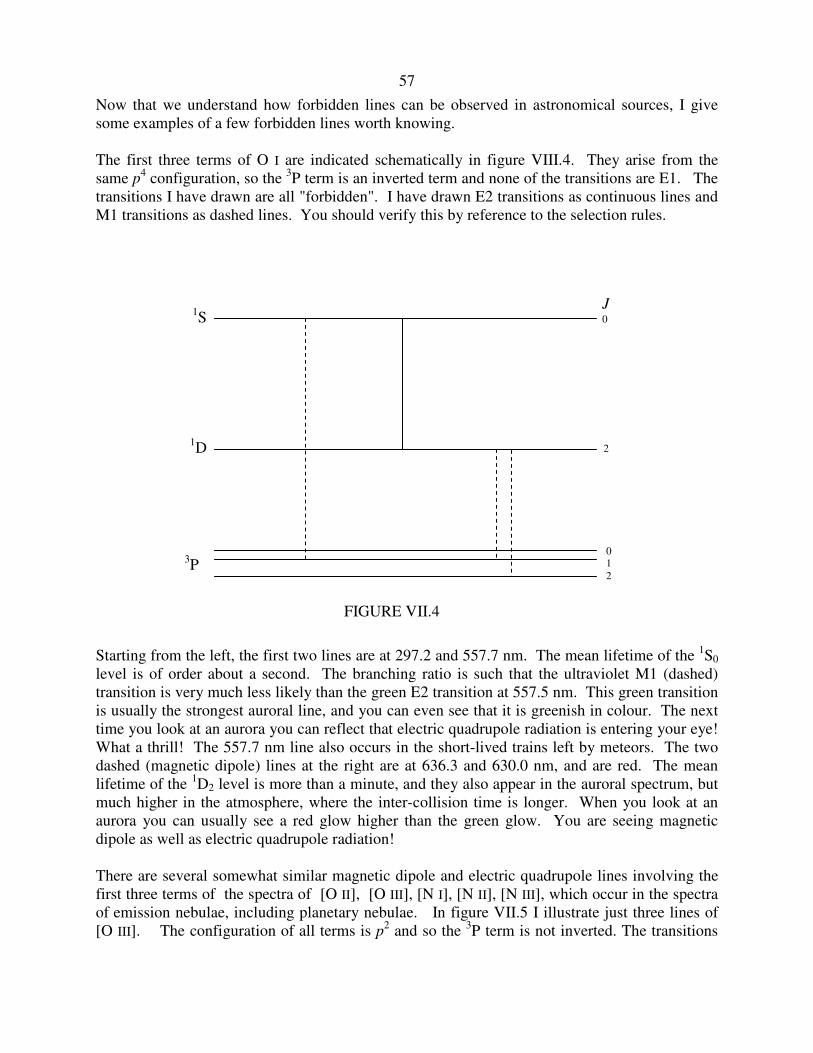
57

Now that we understand how forbidden lines can be observed in astronomical sources, I give some examples of a few forbidden lines worth knowing. The first three terms of O I are indicated schematically in figure VIII.4. They arise from the same p4 configuration, so the 3P term is an inverted term and none of the transitions are E1. The transitions I have drawn are all "forbidden". I have drawn E2 transitions as continuous lines and M1 transitions as dashed lines. You should verify this by reference to the selection rules. Starting from the left, the first two lines are at 297.2 and 557.7 nm. The mean lifetime of the 1S0 level is of order about a second. The branching ratio is such that the ultraviolet M1 (dashed) transition is very much less likely than the green E2 transition at 557.5 nm. This green transition is usually the strongest auroral line, and you can even see that it is greenish in colour. The next time you look at an aurora you can reflect that electric quadrupole radiation is entering your eye! What a thrill! The 557.7 nm line also occurs in the short-lived trains left by meteors. The two dashed (magnetic dipole) lines at the right are at 636.3 and 630.0 nm, and are red. The mean lifetime of the 1D2 level is more than a minute, and they also appear in the auroral spectrum, but much higher in the atmosphere, where the inter-collision time is longer. When you look at an aurora you can usually see a red glow higher than the green glow. You are seeing magnetic dipole as well as electric quadrupole radiation! There are several somewhat similar magnetic dipole and electric quadrupole lines involving the first three terms of the spectra of [O II], [O III], [N I], [N II], [N III], which occur in the spectra of emission nebulae, including planetary nebulae. In figure VII.5 I illustrate just three lines of [O III]. The configuration of all terms is p2 and so the 3P term is not inverted. The transitions

J 0

2

0 1 2

1S

1D

3P

FIGURE VII.4

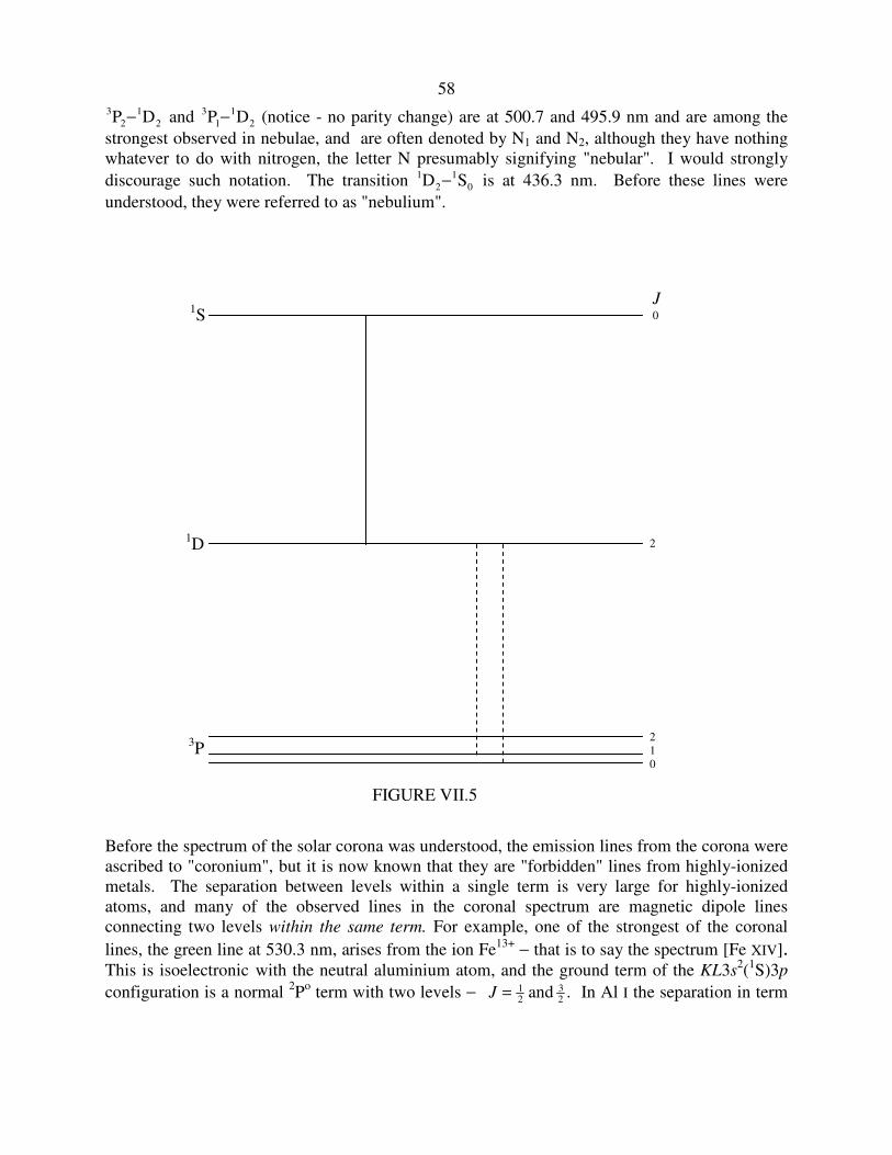
58 3

21

2P D− and 31

12P D− (notice - no parity change) are at 500.7 and 495.9 nm and are among the

strongest observed in nebulae, and are often denoted by N1 and N2, although they have nothing whatever to do with nitrogen, the letter N presumably signifying "nebular". I would strongly discourage such notation. The transition 1

21

0D S− is at 436.3 nm. Before these lines were understood, they were referred to as "nebulium". Before the spectrum of the solar corona was understood, the emission lines from the corona were ascribed to "coronium", but it is now known that they are "forbidden" lines from highly-ionized metals. The separation between levels within a single term is very large for highly-ionized atoms, and many of the observed lines in the coronal spectrum are magnetic dipole lines connecting two levels within the same term. For example, one of the strongest of the coronal lines, the green line at 530.3 nm, arises from the ion Fe13+ − that is to say the spectrum [Fe XIV]. This is isoelectronic with the neutral aluminium atom, and the ground term of the KL3s

2(1S)3p configuration is a normal 2Po term with two levels − J = 1

232and . In Al I the separation in term

J 0

2

2 1 0

1S

1D

3P

FIGURE VII.5

59

value of these levels is only 112 cm-1, but they are much more widely spaced in Fe XIV so that, in this spectrum, the wavelength of 2 2

12

32

P Po− o is 530.3 nm.

The last example is the famous 21-cm transition of neutral hydrogen, H I. Here, the lowest level is 2

12

S , which is the one and only level is the ground term, 2S. The level is split into two

hyperfine levels as a result of the interaction between the total electronic angular momentum ( )2

1=J and the nuclear spin ( )21=I , the F-values of the two hyperfine levels being 0 and 1. The

21-cm line is a magnetic dipole transition between these two hyperfine levels. The nuclear spin of deuterium is I = 1, and consequently the ground level of deuterium is split into hyperfine levels with F = 1

232and . A transition between these two is predicted at 92 cm, but apparently

there is as yet no unambiguous detection of it from an astronomical source.

7.26 Stark Effect

The Stark effect concerns the separation of the states within a level as the result of the application of an external electric field, and the consequent splitting of lines into Stark components. The atmosphere of a star, being hot and highly ionized, is an electrical conductor and consequently cannot sustain electric potential gradients (fields). Thus the splitting of a line into its Stark components is not normally observed in stellar atmospheres, and for that reason I am not going into a detailed description of it or the theory of the effect here. There are just two small points that are probably worth mentioning. The first point concerns the Balmer series of H I. The details of the Stark pattern vary from line to line in the series, but it happens that in every even member of the series, that is to say Hβ, Hδ, etc., there is no central, undisplaced Stark component. Under some circumstances, even if the hydrogen lines are broad and the Stark components are unresolved, this may result in a small dip at the top of an emission line, or a small bump at the bottom of an emission line. There are other effects (see the chapter on line profiles) that can result in a dip at the top of an emission line or a bump at the bottom of an absorption line, but if the cause is Stark splitting, this may be recognized in that it affects only the even members of the Balmer series, and not the odd members (Hα, Hγ, etc.). The second point is that, although a stellar atmosphere cannot sustain a large macroscopic electric field, when two atoms approach each other in a near-collision, each induces a temporary electric dipole on the other. (This is the origin of the van der Waals forces, which fall off inversely as the sixth power of the interatomic distance.) The resulting electric field of one atom on the other, and the other on the one, results in a general broadening of the lines, often asymmetrically, as a result of Stark effect, and this effect obviously increases with pressure and is one of the components of the phenomenon of pressure broadening, to be discussed in a later chapter.

60