1

Chapter 3Chapter 3

Aggregate PlanningAggregate Planning

McGraw-Hill/Irwin Copyright © 2005 by The McGraw-Hill Companies, Inc. All rights reserved.

2

Aggregate Planning StrategiesAggregate Planning Strategies

Should inventories be used to absorb changes in Should inventories be used to absorb changes in demand during planning period?demand during planning period?

Should changes be accomodated by varying the Should changes be accomodated by varying the size of the workforce?size of the workforce?

Should part-timers be used, or should overtime Should part-timers be used, or should overtime and idle time absorb fluctuations?and idle time absorb fluctuations?

Should subcontractors be used on fluctuating Should subcontractors be used on fluctuating orders so a stable workforce can be maintained?orders so a stable workforce can be maintained?

Should prices or other factors be changed to Should prices or other factors be changed to influence demand?influence demand?

3

Introduction to Aggregate PlanningIntroduction to Aggregate Planning

Goal: To plan gross work force levels and set Goal: To plan gross work force levels and set firm-wide production plans.firm-wide production plans.

Concept is predicated on the idea of an Concept is predicated on the idea of an ““aggregate unitaggregate unit” of production: ” of production:

» May be actual units, May be actual units, » May be measured in weight (tons of steel), volume May be measured in weight (tons of steel), volume

(gallons of gasoline), time (worker-hours), or dollars of (gallons of gasoline), time (worker-hours), or dollars of sales. sales.

» Can even be a fictitious quantity. (Refer to example in Can even be a fictitious quantity. (Refer to example in text and in slide below.)text and in slide below.)

4

Overview of the ProblemOverview of the Problem

Suppose that DSuppose that D11, D, D22, . . . , D, . . . , DTT are the forecasts are the forecasts

of demand for aggregate units over the of demand for aggregate units over the planning horizon (T periods.) planning horizon (T periods.)

The problem is to determine both work force The problem is to determine both work force levels (Wlevels (Wtt) and production levels (P) and production levels (Ptt ) to ) to

minimize total costs over the T period minimize total costs over the T period planning horizon. planning horizon.

5

Important IssuesImportant Issues

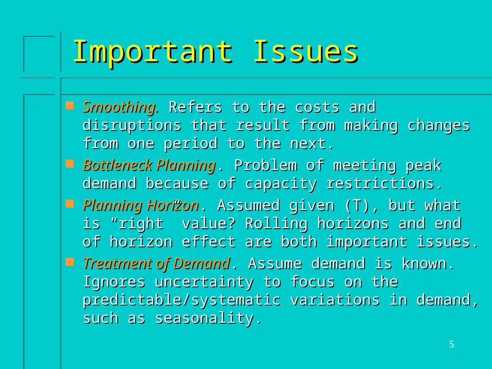
Smoothing.Smoothing. Refers to the costs and disruptions that Refers to the costs and disruptions that result from making changes from one period to the next.result from making changes from one period to the next.

Bottleneck PlanningBottleneck Planning. Problem of meeting peak demand . Problem of meeting peak demand because of capacity restrictions. because of capacity restrictions.

Planning HorizonPlanning Horizon. Assumed given (T), but what is . Assumed given (T), but what is “right” value? Rolling horizons and end of horizon “right” value? Rolling horizons and end of horizon effect are both important issues. effect are both important issues.

Treatment of DemandTreatment of Demand. Assume demand is known. . Assume demand is known. Ignores uncertainty to focus on the Ignores uncertainty to focus on the predictable/systematic variations in demand, such as predictable/systematic variations in demand, such as seasonality.seasonality.

6

Relevant CostsRelevant Costs

Smoothing CostsSmoothing Costs– changing size of the work forcechanging size of the work force– changing number of units producedchanging number of units produced

Holding CostsHolding Costs– primary component: opportunity cost of investmentprimary component: opportunity cost of investment

Shortage CostsShortage Costs– Cost of demand exceeding stock on hand. Why Cost of demand exceeding stock on hand. Why

should shortages be an issue if demand is known? should shortages be an issue if demand is known?

Other Costs:Other Costs: payroll, overtime, subcontracting. payroll, overtime, subcontracting.

7

Aggregate UnitsAggregate Units

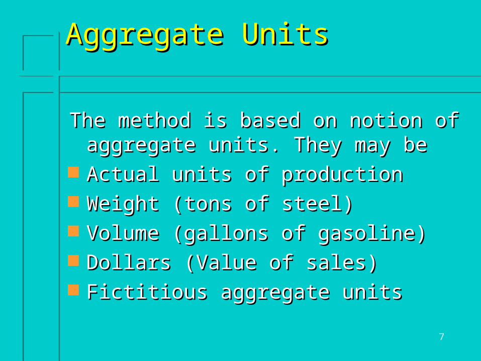
The method is based on notion of aggregate The method is based on notion of aggregate units. They may beunits. They may be

Actual units of productionActual units of production Weight (tons of steel)Weight (tons of steel) Volume (gallons of gasoline)Volume (gallons of gasoline) Dollars (Value of sales)Dollars (Value of sales) Fictitious aggregate unitsFictitious aggregate units

8

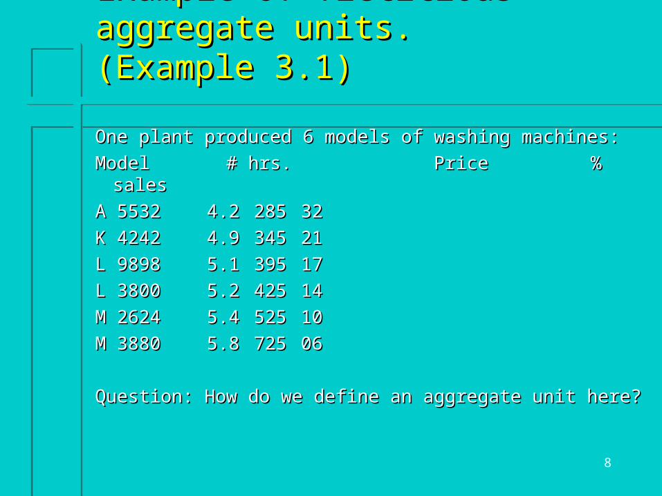
Example of fictitious aggregate units.Example of fictitious aggregate units.(Example 3.1)(Example 3.1)

One plant produced 6 models of washing machines:One plant produced 6 models of washing machines:

Model # hrs. Price Model # hrs. Price % sales % sales

A 5532A 5532 4.24.2 285285 3232

K 4242K 4242 4.94.9 345345 2121

L 9898L 9898 5.15.1 395395 1717

L 3800L 3800 5.25.2 425425 1414

M 2624M 2624 5.45.4 525525 1010

M 3880M 3880 5.85.8 725725 0606

Question: How do we define an aggregate unit here?Question: How do we define an aggregate unit here?

9

Example continuedExample continued

Notice: Price is not necessarily proportional to Notice: Price is not necessarily proportional to worker hours (i.e., cost): why?worker hours (i.e., cost): why?

One method for defining an aggregate unit: One method for defining an aggregate unit: requires: .32(4.2) + .21(4.9) + . . . + .06(5.8) = requires: .32(4.2) + .21(4.9) + . . . + .06(5.8) = 4.8644 worker hours. Forecasts for demand for 4.8644 worker hours. Forecasts for demand for aggregate units can be obtained by taking a aggregate units can be obtained by taking a weighted average (using the same weights) of weighted average (using the same weights) of individual item forecasts. individual item forecasts.

10

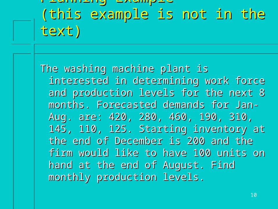
Prototype Aggregate Planning ExamplePrototype Aggregate Planning Example(this example is not in the text)(this example is not in the text)

The washing machine plant is interested in The washing machine plant is interested in determining work force and production levels determining work force and production levels for the next 8 months. Forecasted demands for for the next 8 months. Forecasted demands for Jan-Aug. are: 420, 280, 460, 190, 310, 145, Jan-Aug. are: 420, 280, 460, 190, 310, 145, 110, 125. Starting inventory at the end of 110, 125. Starting inventory at the end of December is 200 and the firm would like to December is 200 and the firm would like to have 100 units on hand at the end of August. have 100 units on hand at the end of August. Find monthly production levels. Find monthly production levels.

11

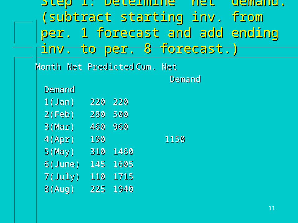
Step 1: Determine “net” demand.Step 1: Determine “net” demand.(subtract starting inv. from per. 1 forecast and (subtract starting inv. from per. 1 forecast and add ending inv. to per. 8 forecast.)add ending inv. to per. 8 forecast.)

MonthMonth Net PredictedNet Predicted Cum. NetCum. Net

Demand DemandDemand Demand

1(Jan)1(Jan) 220220 220220

2(Feb)2(Feb) 280280 500500

3(Mar)3(Mar) 460460 960960

4(Apr)4(Apr) 190190 1150 1150

5(May)5(May) 310310 14601460

6(June)6(June) 145145 16051605

7(July)7(July) 110110 17151715

8(Aug)8(Aug) 225225 19401940

12

Step 2. Graph Cumulative Net Demand Step 2. Graph Cumulative Net Demand to Find Plans Graphicallyto Find Plans Graphically

0

200

400

600

800

1000

1200

1400

1600

1800

2000

1 2 3 4 5 6 7 8

Cum Net Dem

13

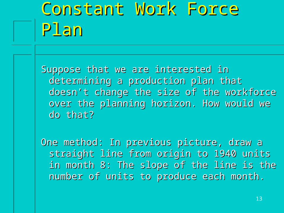
Constant Work Force PlanConstant Work Force Plan

Suppose that we are interested in determining a Suppose that we are interested in determining a production plan that doesn’t change the size of production plan that doesn’t change the size of the workforce over the planning horizon. How the workforce over the planning horizon. How would we do that?would we do that?

One method: In previous picture, draw a straight One method: In previous picture, draw a straight line from origin to 1940 units in month 8: The line from origin to 1940 units in month 8: The slope of the line is the number of units to slope of the line is the number of units to produce each month.produce each month.

14

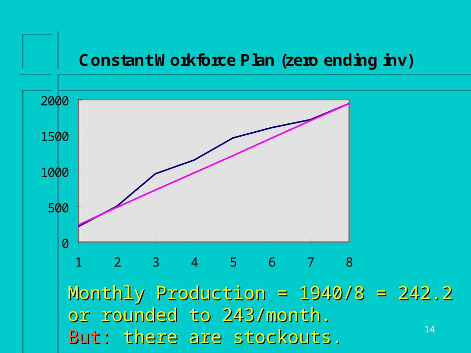
Constant Workforce Plan (zero ending inv)

0

500

1000

1500

2000

1 2 3 4 5 6 7 8

Monthly Production = 1940/8 = 242.2 or rounded to Monthly Production = 1940/8 = 242.2 or rounded to 243/month. 243/month. But:But: there are stockouts. there are stockouts.

15

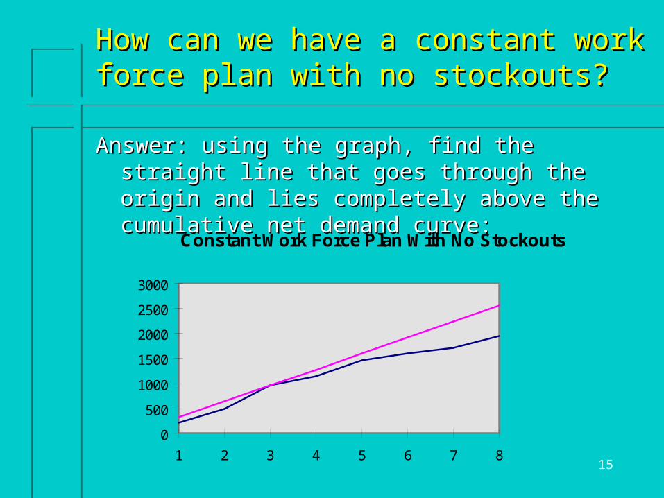
How can we have a constant work force plan How can we have a constant work force plan with no stockouts?with no stockouts?

Answer: using the graph, find the straight line that goes Answer: using the graph, find the straight line that goes through the origin and lies completely above the through the origin and lies completely above the cumulative net demand curve:cumulative net demand curve:

Constant Work Force Plan With No Stockouts

0

500

1000

1500

2000

2500

3000

1 2 3 4 5 6 7 8

16

From the previous graph, we see that cum. net demand curve From the previous graph, we see that cum. net demand curve is crossed at period 3, so that monthly production is 960/3 = is crossed at period 3, so that monthly production is 960/3 = 320. Ending inventory each month is found from:320. Ending inventory each month is found from:

Month Cum. Net. Dem. Cum. Prod. Invent.Month Cum. Net. Dem. Cum. Prod. Invent.

1(Jan)1(Jan) 220220 320 320 100 100

2(Feb)2(Feb) 500 640 140500 640 140

3(Mar)3(Mar) 960 960 0960 960 0

4(Apr.) 1150 1280 1304(Apr.) 1150 1280 130

5(May)5(May) 1460 1600 140 1460 1600 140

6(June)6(June) 1605 1920 315 1605 1920 315

7(July)7(July) 1715 2240 525 1715 2240 525

8(Aug)8(Aug) 1940 2560 620 1940 2560 620

17

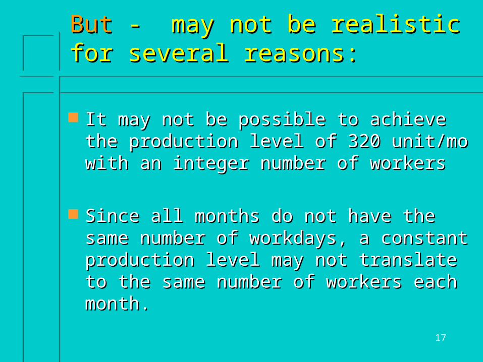
ButBut - may not be realistic for several - may not be realistic for several reasons:reasons:

It may not be possible to achieve the It may not be possible to achieve the production level of 320 unit/mo with an production level of 320 unit/mo with an integer number of workersinteger number of workers

Since all months do not have the same Since all months do not have the same number of workdays, a constant production number of workdays, a constant production level may not translate to the same number level may not translate to the same number of workers each month.of workers each month.

18

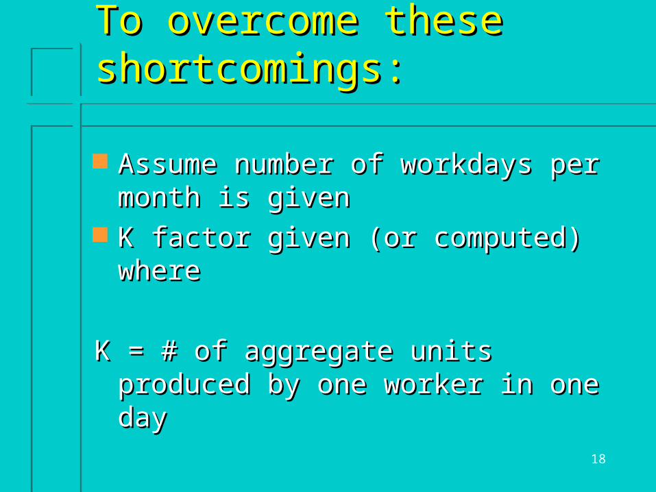
To overcome these shortcomings:To overcome these shortcomings:

Assume number of workdays per month is Assume number of workdays per month is givengiven

K factor given (or computed) where K factor given (or computed) where

K = # of aggregate units produced by one K = # of aggregate units produced by one worker in one dayworker in one day

19

Finding KFinding K

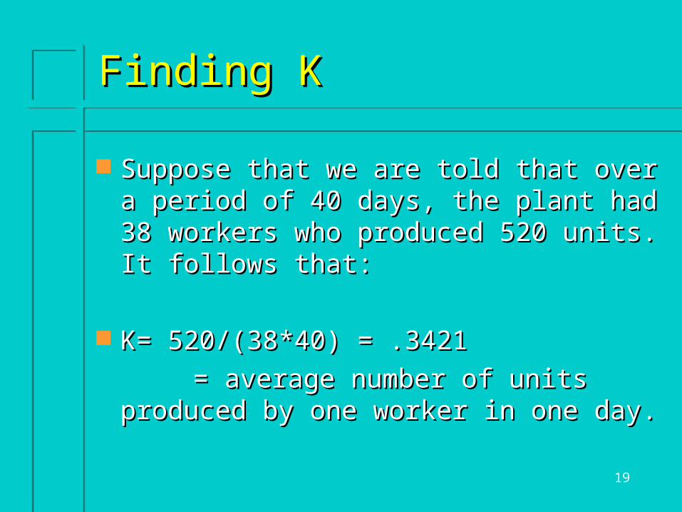
Suppose that we are told that over a period Suppose that we are told that over a period of 40 days, the plant had 38 workers who of 40 days, the plant had 38 workers who produced 520 units. It follows that:produced 520 units. It follows that:

K= 520/(38*40) = .3421 K= 520/(38*40) = .3421

= average number of units produced by = average number of units produced by one worker in one day.one worker in one day.

20

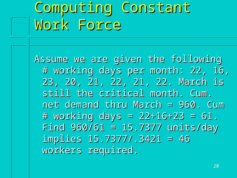
Computing Constant Work ForceComputing Constant Work Force

Assume we are given the following # working Assume we are given the following # working days per month: 22, 16, 23, 20, 21, 22, 21, days per month: 22, 16, 23, 20, 21, 22, 21, 22. March is still the critical month. Cum. 22. March is still the critical month. Cum. net demand thru March = 960. Cum # net demand thru March = 960. Cum # working days = 22+16+23 = 61. Find working days = 22+16+23 = 61. Find 960/61 = 15.7377 units/day implies 960/61 = 15.7377 units/day implies 15.7377/.3421 = 46 workers required.15.7377/.3421 = 46 workers required.

21

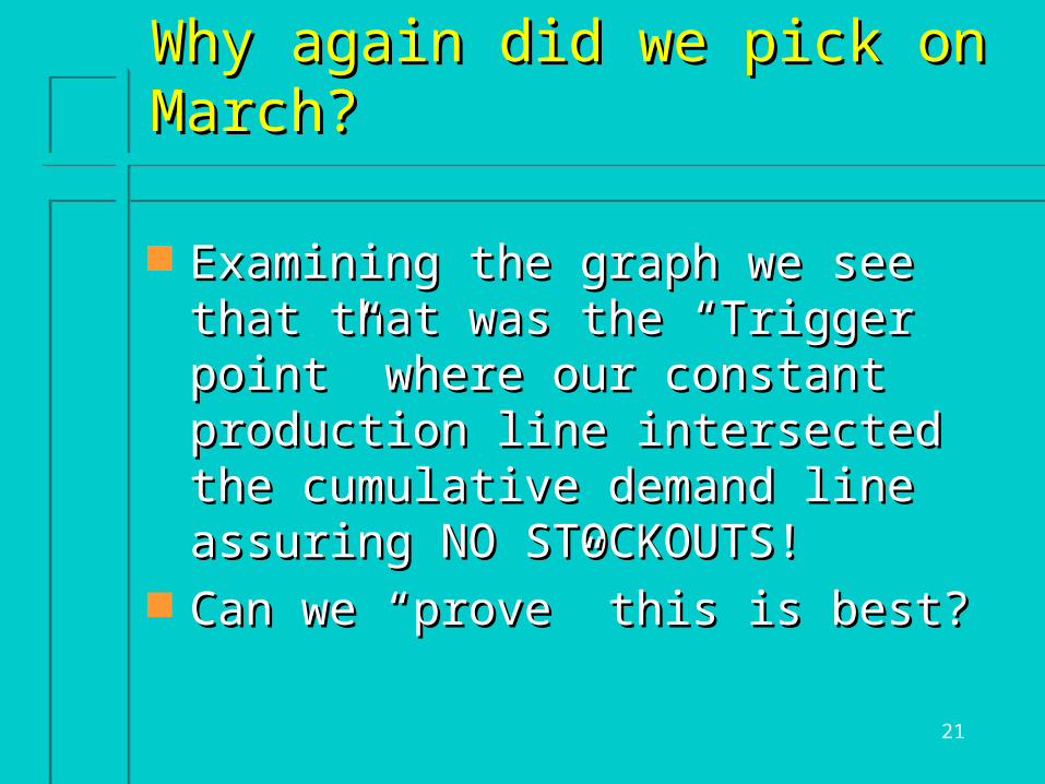
Why again did we pick on March?Why again did we pick on March?

Examining the graph we see that that was Examining the graph we see that that was the “Trigger point” where our constant the “Trigger point” where our constant production line intersected the cumulative production line intersected the cumulative demand line assuring NO STOCKOUTS!demand line assuring NO STOCKOUTS!

Can we “prove” this is best?Can we “prove” this is best?

22

Tabulate Days/Production per Worker Vs. Tabulate Days/Production per Worker Vs. Demand to find minimum numbersDemand to find minimum numbers

Month # Work Days #Units/worker Forecast Demand net Min # Workers C. Net Demand C.Units/WorkerMin #

Workers

Jan 22.00 7.53 220.00 29.23 220.00 7.53 29.23

Feb 16.00 5.47 280.00 51.15 500.00 13.00 38.46

Mar 23.00 7.87 460.00 58.46 960.00 20.87 46.00

Apr 20.00 6.84 190.00 27.77 1150.00 27.71 41.50

May 21.00 7.18 310.00 43.15 1460.00 34.89 41.84

Jun 22.00 7.53 145.00 19.27 1605.00 42.42 37.84

Jul 21.00 7.18 110.00 15.31 1715.00 49.60 34.57

Aug 22.00 7.53 225.00 29.90 1940.00 57.13 33.96

23

What should we look at?What should we look at?

Cumulative Demand says March needs Cumulative Demand says March needs most workers – but will mean building most workers – but will mean building inventories in Jan + Feb inventories in Jan + Feb

If we keep this number of workers we will If we keep this number of workers we will continue to build inventory through the rest continue to build inventory through the rest of the planof the plan

24

Constant Work Force Production PlanConstant Work Force Production Plan

MoMo # wk days Prod. Cum Cum Nt End Inv # wk days Prod. Cum Cum Nt End Inv

Level Prod DemLevel Prod Dem

Jan 22 346 346 220 126Jan 22 346 346 220 126

Feb 16 252 598 500 98Feb 16 252 598 500 98

Mar 23 362 960 960 0Mar 23 362 960 960 0

Apr 20 315 1275 1150 125Apr 20 315 1275 1150 125

May 21 330 1605 1460 145May 21 330 1605 1460 145

Jun 22 346 1951 1605 346Jun 22 346 1951 1605 346

Jul 21 330 2281 1715 566Jul 21 330 2281 1715 566

Aug 22 346 2627 1940 687Aug 22 346 2627 1940 687

25

Addition of CostsAddition of Costs

Holding Cost (per unit per month): $8.50Holding Cost (per unit per month): $8.50 Hiring Cost per worker: $800Hiring Cost per worker: $800 Firing Cost per worker: $1,250Firing Cost per worker: $1,250 Payroll Cost: $75/worker/dayPayroll Cost: $75/worker/day Shortage Cost: $50 unit short/monthShortage Cost: $50 unit short/month

26

Cost Evaluation of Constant Work Force PlanCost Evaluation of Constant Work Force Plan

Assume that the work force at end of Dec was 40.Assume that the work force at end of Dec was 40. Cost to hire 6 workers: 6*800 = $4800Cost to hire 6 workers: 6*800 = $4800 Inventory Cost: accumulate ending inventory: Inventory Cost: accumulate ending inventory:

(126+98+0+. . .+687) = 2093. Add in 100 units netted (126+98+0+. . .+687) = 2093. Add in 100 units netted out in Aug = 2193. Hence Inv. Cost = out in Aug = 2193. Hence Inv. Cost = 2193*8.5=$18,640.502193*8.5=$18,640.50

Payroll cost: Payroll cost:

($75/worker/day)(46 workers )(167days) = $576,150($75/worker/day)(46 workers )(167days) = $576,150 Cost of plan: $576,150 + $18,640.50 + $4800 = Cost of plan: $576,150 + $18,640.50 + $4800 =

$599,590.50$599,590.50

27

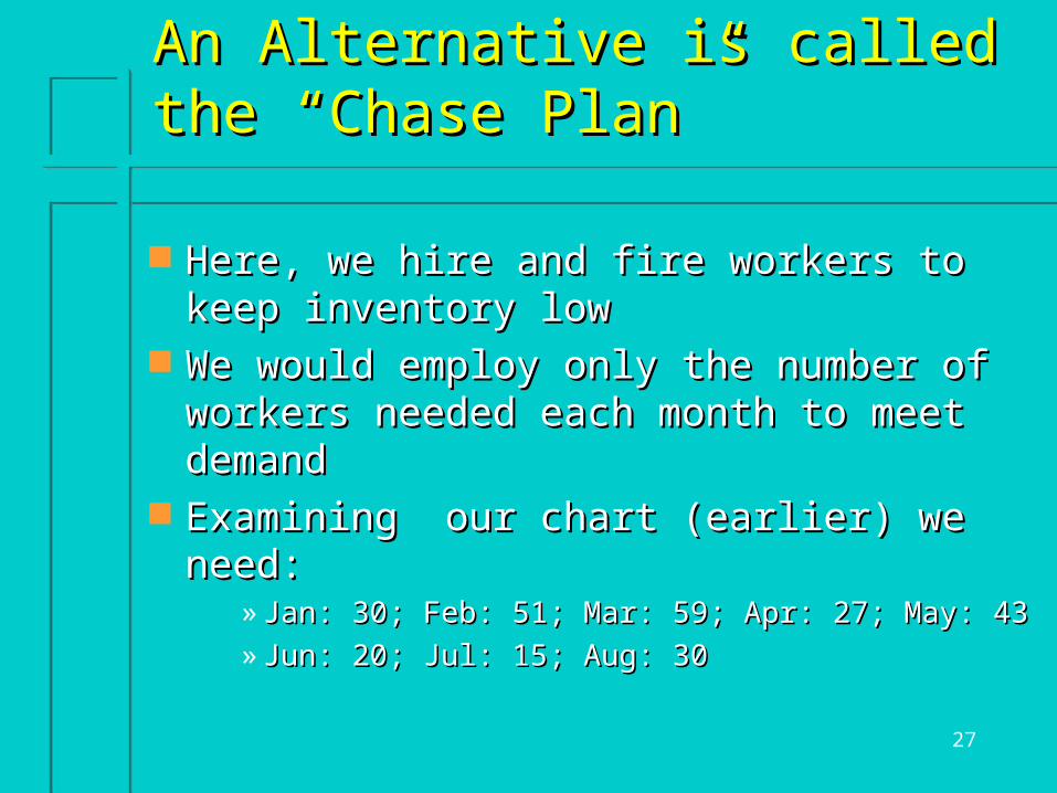
An Alternative is called the “Chase An Alternative is called the “Chase Plan”Plan”

Here, we hire and fire workers to keep Here, we hire and fire workers to keep inventory lowinventory low

We would employ only the number of We would employ only the number of workers needed each month to meet workers needed each month to meet demanddemand

Examining our chart (earlier) we need:Examining our chart (earlier) we need:» Jan: 30; Feb: 51; Mar: 59; Apr: 27; May: 43Jan: 30; Feb: 51; Mar: 59; Apr: 27; May: 43

» Jun: 20; Jul: 15; Aug: 30Jun: 20; Jul: 15; Aug: 30

28

An Alternative is called the “Chase An Alternative is called the “Chase Plan”Plan”

So we hire or Fire (lay-off) monthlySo we hire or Fire (lay-off) monthly» Jan (starts with 40 workers): Fire 10 (cost $8000)Jan (starts with 40 workers): Fire 10 (cost $8000)

» Feb: Hire 21 (cost $16800)Feb: Hire 21 (cost $16800)

» Mar: Hire 8 (cost $6400)Mar: Hire 8 (cost $6400)

» Apr: Fire 31 (cost $38750)Apr: Fire 31 (cost $38750)

» May: Hire 15 (cost $12000)May: Hire 15 (cost $12000)

» Jun: Fire 23 (cost $28750)Jun: Fire 23 (cost $28750)

» Jul: Fire 5 (cost $6250)Jul: Fire 5 (cost $6250)

» Aug: Hire 15 (cost $12000)Aug: Hire 15 (cost $12000)

Total Personnel Costs: $128950Total Personnel Costs: $128950

29

An Alternative is called the “Chase An Alternative is called the “Chase Plan”Plan”

Inventory cost is essentially 165*8.5 = Inventory cost is essentially 165*8.5 = $1402.50$1402.50

Employment costs: $428325Employment costs: $428325 Chase Plan Total: $558677.50Chase Plan Total: $558677.50 Betters the “Constant Workforce Plan” by:Betters the “Constant Workforce Plan” by:

» 599590.50 – 558677.50 = 40913599590.50 – 558677.50 = 40913

But will this be good for your image?But will this be good for your image? Can we find a better plan?Can we find a better plan?

30

Cost Reduction in Constant Work Force Plan Cost Reduction in Constant Work Force Plan & Chase Plan& Chase Plan

In the original cum net demand curve, consider making In the original cum net demand curve, consider making reductions in the work force one or more times over the reductions in the work force one or more times over the

planning horizon to decrease inventory investmentplanning horizon to decrease inventory investment..

Plan Modified With Lay Offs in March and May

0

500

1000

1500

2000

1 2 3 4 5 6 7 8

31

Cost Evaluation of Modified PlanCost Evaluation of Modified Plan

I will not present all the details here. The I will not present all the details here. The modified plan calls for reducing the modified plan calls for reducing the workforce to 36 at start of April and making workforce to 36 at start of April and making another reduction to 22 at start of June. The another reduction to 22 at start of June. The additional cost of layoffs is $30,000, but additional cost of layoffs is $30,000, but holding costs are reduced to only $4,250. holding costs are reduced to only $4,250. The total cost of the modified plan is The total cost of the modified plan is $467,450. $467,450.

32

Optimal Solutions to Aggregate Planning Optimal Solutions to Aggregate Planning Problems Via Linear ProgrammingProblems Via Linear Programming

Linear Programming provides a means of solving Linear Programming provides a means of solving aggregate planning problems optimally. The LP aggregate planning problems optimally. The LP formulation is fairly complex requiring 8T formulation is fairly complex requiring 8T variables and 3T constraints, where T is the length variables and 3T constraints, where T is the length of the planning horizon. Clearly, this can be a of the planning horizon. Clearly, this can be a formidable linear program. The LP formulation formidable linear program. The LP formulation shows that the modified plan we considered with shows that the modified plan we considered with two months of layoffs is in fact optimal for the two months of layoffs is in fact optimal for the prototype problem.prototype problem.

33

Exploring the Optimal (L.P.) Exploring the Optimal (L.P.) ApproachApproach

We need an Objective Function for cost of the aggregate We need an Objective Function for cost of the aggregate plan (target minimization):plan (target minimization):

– Here the cHere the cii’s are cost for hiring, firing, inventory, production, ’s are cost for hiring, firing, inventory, production,

etcetc

– HHTT and F and FTT are number of workers hired and fired are number of workers hired and fired

– IITT, P, PTT, O, OTT, S, STT AND U AND UTT are numbers inventoried, produced on are numbers inventoried, produced on

regular time, overtime, by ‘sub-contract’ or idle worker hours regular time, overtime, by ‘sub-contract’ or idle worker hours respectivelyrespectively

1

T

H H F F I T R R o T u T S Tt

c N c N c I c P c O c U c S

34

Exploring the Optimal (L.P.) Exploring the Optimal (L.P.) ApproachApproach

This objective Function would be subject to This objective Function would be subject to a series of constraints (one for each period)a series of constraints (one for each period)– Number of Worker Constraints:Number of Worker Constraints:

– Inventory Constraints:Inventory Constraints:

– Production Constraints:Production Constraints:

1t t t tW W H F

1t t t t tI I P S D

Where: k*n is the number of units produced by a worker t

on regular time during a period

t t t t tP k n W O U

35

Exploring the Optimal (L.P.) Exploring the Optimal (L.P.) ApproachApproach

Assuming we allow no idle time and will produce Assuming we allow no idle time and will produce only on regular timeonly on regular time

» No overtime or subcontractingNo overtime or subcontracting

We would have:We would have:» 9 worker variables (W9 worker variables (W00 to W to Waugaug))» 8 Hire Variable8 Hire Variable» 8 Fire Variables8 Fire Variables» 9 Inventory Variables (I9 Inventory Variables (I00 to I to Iaugaug))» 8 Production Variables8 Production Variables» 8 ‘Demands’8 ‘Demands’» And 1 complicated Objective functionAnd 1 complicated Objective function

36

Exploring the Optimal (L.P.) Exploring the Optimal (L.P.) ApproachApproach

Lets try Excel!Lets try Excel! This is a toughee!This is a toughee! Lots of variables and lots of constraints – Lots of variables and lots of constraints –

but work is straight forward!but work is straight forward!

37

DisaggregationDisaggregation

Aggregate plans were built to optimal staffing Aggregate plans were built to optimal staffing levels for “families” or groups of productslevels for “families” or groups of products

Disaggregation is a means to build specific Disaggregation is a means to build specific “Master Production Schedules”“Master Production Schedules”

Typically by breaking down the aggregating Typically by breaking down the aggregating weights to individual parts – or working on weights to individual parts – or working on schedules of these families as optimal schedules of these families as optimal

Later leads to values similar to EOQ which we Later leads to values similar to EOQ which we will explore in Chapter 4!will explore in Chapter 4!