1

CGILS: First Results from an International Project to Understand the Physical Mechanisms of 2

Low Cloud Feedbacks in General Circulation Models 3

4

Minghua Zhang, Christopher S. Bretherton, Peter N. Blossey, Phillip A. Austin, Julio T. Bacmeister, 5

Sandrine Bony, Florent Brient, Anning Cheng, Stephan R. De Roode, Satoshi Endo, Anthony D. Del 6

Genio, Charmaine N. Franklin, Jean-Christophe Golaz, Cecile Hannay, Thijs Heus, Francesco 7

Alessandro Isotta, Dufresne Jean-Louis, In-Sik Kang, Hideaki Kawai, Martin Koehler, Suvarchal 8

Kumar, Vincent E. Larson, Yangang Liu, Adrian Lock, Ulrike Lohman, Marat F. Khairoutdinov, 9

Andrea M. Molod, Roel A.J. Neggers, Philip Rasch, Irina Sandu, Ryan Senkbeil, A. Pier Siebesma, 10

Colombe Siegenthaler-Le Drian, Bjorn Stevens, Max J. Suarez, Kuan-Man Xu, Knut von Salzen, 11

Mark Webb, Audrey Wolf, Ming Zhao 12

13

Bulletin of American Meteorological Society 14

(Manuscript# BAMS-D-12-00140) 15

July 2012 16

Revised March 2013 17

18

CORRESPONDING AUTHOR: 19

Minghua Zhang, Institute for Terrestrial and Planetary Atmospheres, Stony Brook University, Stony 20

Brook, NY 11794-5000. Email: minghua.zhang@stonybrook.edu 21

1

AFFILIATIONS: 22 23

Minghua Zhang and Marat F. Khairoutdinov 24 Stony Brook University 25

26 Christopher S. Bretherton and Peter N. Blossey 27

University of Washington 28 29

Phillip A. Austin 30 University of British Columbia 31

32

Julio T. Bacmeister and Cecile Hannay 33 National Center for Atmospheric Research 34

35

Sandrine Bony, Florent Brient, and Jean-Louis Dufresne 36 Laboratoire de Meteorologie Dynamique/Institute Pierre Simon Laplace (IPSL), France 37

38

Anning Cheng, Kuan-Man Xu 39 NASA Langley Research Center 40

41

Anthony D. Del Genio 42 NASA Goddard Institute for Space Studies 43

44 Stephan R. de Roode 45

Delft University of Technology, The Netherlands 46 47

Satoshi Endo and Yangang Liu 48 Brookhaven National Laboratory 49

50 Charmaine N. Franklin 51

Centre for Australian Weather and Climate Research, Commonwealth Scientific and Industrial 52 Research Organisation (CSIRO), Australia 53

54

Jean-Christophe Golaz and Ming Zhao 55 NOAA Geophysical Fluid Dynamics Laboratory 56

57 Thijs Heus, Suvarchal K. Cheedela, Irina Sandu and Bjorn Stevens 58

Max Planck Institute for Meteorology, Hamburg, Germany 59

60

Francesco Alessandro Isotta, Ulrike Lohman and Colombe Siegenthaler-Le Drian 61 Swiss Federal Institute of Technology, Switzerland 62

63

In-Sik Kang 64 Seoul National University, Korea 65

66

2

Hideaki Kawai 67 Meteorological Research Institute, Japan. 68

69 Martin Koehler 70

European Centre for Medium-Range Weather Forecasts 71 72

Vincent E. Larson and Ryan Senkbeil 73 University of Wisconsin 74

75

Adrian Lock and Mark Webb 76 Met Office, United Kingdom 77

78 Andrea M. Molod and Max J. Suarez 79

NASA Goddard Space Flight Center 80 81

Roel A.J. Neggers, and A. Pier Siebesma 82 Royal Netherlands Meteorological Institute (KNMI), the Netherlands 83

84 Philip Rasch 85

Pacific Northwest National Laboratory 86 87

Knut von Salzen 88 Canadian Centre for Climate Modelling and Analysis, Canada 89

90

Audrey Wolf 91 Columbia University 92

93 94

95

3

96

97

98

99

CAPSULE SUMMARY 100

101

Single Column Models (SCM) and Large Eddy Models (LES) and are used in an idealized climate 102

change scenario to investigate the physical mechanism of low cloud feedbacks in models. Enhanced 103

moistening from surface-driven boundary layer turbulence and enhanced drying from shallow 104

convection in a warmer climate are found to be the two dominant opposing mechanisms of low cloud 105

feedbacks in SCMs. 106

107

4

ABSTRACT 108

CGILS – the CFMIP-GASS Intercomparison of Large Eddy Models (LESs) and Single 109

Column Models (SCMs) – is an international project in which most major climate modeling centers 110

participated to investigate the mechanisms of cloud feedback in SCMs and LESs under idealized 111

climate change perturbation. This paper describes the CGILS project and results from 15 SCMs and 112

eight LES models. Three cloud regimes over the subtropical oceans are studied: shallow cumulus, 113

cumulus under stratocumulus, and well-mixed coastal stratus/stratocumulus. SCMs simulated a wide 114

range of cloud feedbacks in all regimes. In the stratocumulus and coastal stratus regimes, models 115

without active shallow convection tend to simulate negative cloud feedbacks, while models with active 116

shallow convection tend to simulate positive cloud feedbacks. In the shallow cumulus regime, this 117

relationship is less clear, likely due to the larger cloud depth and different parameterization of lateral 118

mixing of clouds. The majority of LES models simulated positive cloud feedback in the shallow 119

cumulus and stratocumulus regime, and negative cloud feedback in the well-mixed coastal 120

stratus/stratocumulus regime. A general framework is provided to interpret SCM results. In a 121

warmer climate, there is enhanced moistening of the cloudy layer by the surface-based turbulence 122

parameterization, which alone causes negative cloud feedback, while there is enhanced drying by the 123

shallow convection scheme or cloud-top entrainment parameterization, which alone tends to cause 124

positive low cloud. The net cloud feedback depends on how these two opposing effects counteract 125

each other. These results highlight the need to treat physical parameterizations in General Circulation 126

Models (GCMs) as systems rather than individual components. 127

128

5

129

1. Introduction 130

Cloud-climate feedbacks in General Circulation Models (GCMs) have been the subject of 131

intensive study for the last four decades (e.g., Randall et al. 2007). These feedbacks were identified 132

to be one of the most significant uncertainties in projecting future global warming in past IPCC (Inter-133

Governmental Panel for Climate Change) Assessment Reports (AR), as well as in coupled model 134

simulations that will be used for the upcoming AR5 (Andrews et al. 2012). Despite of many progress 135

toward understanding cloud feedbacks (Stephens 2005; Bony et al. 2006), however, there is still a 136

general lack of knowledge about their mechanisms. Understanding the physical mechanisms is 137

necessary to instill our confidence in the sensitivity of climate models. 138

Cloud-climate feedbacks refer to the radiative impact of changes of clouds on climate change. 139

Because clouds are not explicitly resolved in GCMs, they are the product of an interactive and 140

elaborate suite of physical parameterizations. As a result, it has been a challenge to decipher cloud 141

feedback mechanisms in climate models. Clouds also interact with the resolved-scale atmospheric 142

dynamical circulations through their impact on latent and radiative heating. 143

In view of the challenges, CFMIP (the Cloud Feedback Model Intercomparison Project) and 144

GASS (GEWEX (Global Energy and Water Cycle Experiment) Atmospheric System Study) initiated a 145

joint project -- CGILS (the CFMIP-GASS Intercomparison of Large Eddy Models (LESs) and Single 146

Column Models (SCMs)) to analyze the physical mechanisms of cloud feedbacks by using a 147

simplified experimental setup. The focus of CGILS is on low clouds in the subtropics, because 148

several studies have demonstrated that these clouds contribute significantly to cloud feedback 149

differences in models (e.g., Bony and Dufresne 2005; Zelinka et al. 2012). The role played by these 150

6

clouds is consistent with the fact that low clouds have the largest net cloud radiative effect, in contrast 151

to deep clouds in which the positive longwave and negative shortwave cloud effects largely cancel out 152

(e.g. Ramanathan et al. 1989). 153

The objective of this paper is to describe the CGILS project and results from 15 SCMs and 154

eight LES models. The paper is organized as follows. Section 2 describes the experimental design 155

and large-scale forcing data. Section 3 gives a brief description of the participating models. Section 156

4 discusses simulated clouds and the associated physical processes. Section 5 discusses cloud feedback 157

results. The last section is a brief summary. 158

2. Experimental Design and Large-Scale Forcing Data 159

a. Experimental design 160

Figure 1 shows the schematics of the CGILS experimental design modified from Zhang and 161

Bretherton (2008). In the control climate (CTL), sea surface temperature (SST) is specified along the 162

GCSS/WGNE Pacific Cross Section Intercomparison (GPCI) (Teixeira et al. 2011) in the northeast 163

Pacific by using the ECMWF (European Center for Medium-Range Weather Forecasts) Interim 164

Reanalysis (Dee et al. 2011, ERA-Interim). In the perturbed climate (P2S), SST is uniformly raised 165

everywhere by 2 degrees as in Cess et al. (1990). Large-scale horizontal advection and vertical 166

motion, corresponding to the underlying SST, are derived and used to force SCMs and LES models. 167

The models simulate changes of clouds in response to changes of SST and the associated large-scale 168

atmospheric conditions. 169

Three locations along the GPCI cross section are selected for study. They are labeled as S6, 170

S11 and S12 in Figure 2, which also shows the distribution of low cloud amount in the summer (JJA, 171

7

June to August) from satellites (Kato et al. 2011; Xu and Cheng 2012). Typical regimes of clouds at 172

these three locations are shallow cumulus (S6), cumulus under or above stratocumulus (S11), and 173

well-mixed stratocumulus or coastal stratus (S12). On the basis of dominant cloud types, they are 174

referred to as shallow cumulus, stratocumulus, and coastal stratus respectively. Table 1 gives the 175

locations and values of summer-time surface meteorological variables in the control climate. 176

b. Forcing data 177

The SCM and LES forcing data refer to surface boundary conditions, the large-scale horizontal 178

advective tendencies and vertical velocity that are specified in the model simulations. The SCMs 179

calculate the time evolution of water vapor and temperature as follows (Randall and Cripe 1999): 180

pV

tt

mLSLSphy

mm

)()(

(1) 181

p

qqV

t

q

t

q mLSLSphy

mm

)()(

, (2) 182

where and q are potential temperature and water vapor mixing ratio. Subscript “m” denotes 183

model calculations; “LS” stands for large-scale; other symbols are as commonly used. The first term 184

on the right-hand-side (rhs) of Equations (1)-(2) is calculated from physical parameterizations (with 185

subscript “phys”). The last two terms contain the specified large-scale horizontal advective forcing 186

and subsidence. In LES models, conservative variables like liquid water potential temperature and 187

total liquid water are typically used as prognostic fields (e.g., Siebesma et al. 2004; Stevens et al. 188

2005); (1) and (2) represent domain averages. The atmospheric winds and initial relative humidity 189

are specified by using the ERA-Interim for July 2003. Initial profiles of atmospheric temperature are 190

8

assumed to follow moist adiabat over the warm pool and weak gradient approximations at other 191

locations (Sobel et al. 2001). Surface latent and sensible heat fluxes are calculated internally by each 192

model from the specified SST and winds. 193

The large-scale horizontal advective tendencies and subsidence in (1)-(2) are specified 194

according to SST. In the free troposphere, they are derived based on the clear-sky thermodynamic 195

and water vapor mass continuity equations, in which radiative cooling in the thermodynamic equation 196

is balanced by subsidence warming and horizontal advection, with the radiative cooling calculated by 197

using the RRTM radiation code (Mlawer et al. 1997). Below the altitude of 900 hPa, the horizontal 198

advective forcing of temperature and water vapor are calculated using the SST spatial gradient and 199

specified surface relative humidity. A brief description of the derivation procedure is given in 200

Appendix A. More detailed discussions of the forcing data can be found in Zhang et al. (2012). 201

Figure 3a shows the derived vertical profiles of LS in CGILS CTL (solid lines) and ERA-202

Interim (dashed lines) at the three chosen locations. The obtained values match well with ERA-203

Interim in the lower troposphere. Among the three locations, the subsidence rate is the strongest at 204

S12 and the weakest at S6. 205

Figure 3b shows the comparison of the derived LS between CTL (solid lines) and P2S 206

(dashed lines) used in the simulations. It is seen that subsidence is weaker in the warmer climate. 207

Figures 3c and 3d show the corresponding profiles of horizontal advective tendencies of temperature 208

and water vapor respectively. in the free troposphere, these profiles, along with the profiles of LS , 209

SST, and initial atmospheric temperature and water vapor, satisfy the clear-sky atmospheric 210

thermodynamic and water vapor mass continuity equations under July 15 insolation conditions. 211

9

Zhang et al. (2012) showed that the changes in the forcing data between CTL and P2S in Figure 3 212

capture the essential features in the GCMs. All data are available in the CGILS website 213

http://atmgcm.msrc.sunysb.edu/cfmip_figs/Case_specification.html. 214

c. Simulations 215

We use the change of cloud-radiative forcing (CRF) (Ramanathan et al. 1989) from CTL to 216

P2S, as in many previous studies, to measure cloud feedbacks. Even though Soden et al. (2004) 217

suggested other better diagnostics of cloud feedbacks, CRF is used for simplicity, which should not 218

affect the results of this paper. 219

The SCMs and LES are integrated to quasi-equilibrium states by using the same steady large-220

scale advective tendencies and subsidence as forcing data. Each model ran six simulations: CTL and 221

P2S at the three locations of S6, S11 and S12. Since the forcing is fixed, a model may eventually 222

drift if its radiative cooling rate in the free atmosphere differs from the rate used in the derivation of 223

the prescribed large-scale subsidence. To prevent models from similar drifting, at pressure less than 224

600 hPa, temperature and water vapor mixing ratio are relaxed to their initial conditions with a time 225

scale of 3 hours. In LES models, they are relaxed at altitudes above 4000 m for S6, 2500 m for S11, 226

and 1200 m for S12, respectively to reduce computational costs and allow for high vertical resolutions 227

in shallow domains. Some LES models did not complete all six simulations. 228

Most of the SCMs are integrated for 100 days. Based on a visual inspection of statistical 229

equilibrium, the averages of their last period of about 50 days are used. Most LES simulations 230

reached quasi-equilibrium states after 10 days, in which case the last two days are used in the analysis. 231

Zhang and Bretherton (2008) analyzed the transient behavior of the Community Atmospheric Model 232

10

(CAM) under constant forcing and showed that the interaction of different physical parameterization 233

components can create quasi-periodic behaviors of model simulation with time scales longer than a 234

day. Since LES models contain fewer parameterization components, the impact of this type of 235

interactions is reduced. This likely explains why LES models reach quasi-steady states in shorter time 236

than SCMs. To our knowledge, CGILS is the first LES intercomparion study to investigate clouds by 237

integrating them to quasi-equilibrium states. 238

3. Models and Differences in Physical Parameterizations 239

Fifteen SCMs and eight LES models participated in this study. Many parent GCMs of the 240

SCMs also participated in the Coupled Model Intercomparison Project 5 (CMIP5). Table 2 lists the 241

model names, main references, and CGILS contributors. It also gives the number of total vertical 242

model layers and number of layers between the surface and 700 hPa in SCMs. The SCM vertical 243

resolution in the boundary layer (PBL) is generally not sufficient to resolve observed thin clouds. No 244

attempt is made to make them finer since our objective is to understand the behavior of operational 245

GCMs. For the LES models, however, because they are intended as benchmarks, much higher 246

resolutions are used. The horizontal resolutions of LES models are 100 meter, 50 meter and 25 meter 247

respectively at S6, S11 and S12. The vertical resolutions of the majority of LES are 40 meter, 5 248

meter and 5 meter respectively at the three locations. More detailed descriptions of the CGILS LES 249

models are given in a recent paper by Blossey et al. (2013). 250

The physical parameterizations in the SCMs relevant to the present study are the PBL, shallow 251

convection, and cloud schemes. Cloud schemes include a macrophysical and a microphysical 252

component. For PBL schemes, the generic form can be written in terms of turbulent flux at the 253

model interfaces: 254

11

)('' ccz

SKSw

(3) 255

where z is height; w is vertical velocity; S is a conservative model prognostic variable. Prime 256

represents the turbulent perturbation from the mean that is denoted by the overbar. Kc is the eddy 257

diffusivity, and c is the counter-gradient transport term. In addition to resolution, the differences 258

in PBL schemes among the models are in their formulations of Kc and c . For Kc, some models 259

parameterize it by using local variables at the resolved scales, such as local Richardson number in the 260

so-called first order closure models, or local turbulent eddy kinetic energy (TKE) such as the Mellor-261

Yamada higher order closure models (Mellor and Yamada 1974). Other models use non-local 262

empirical parameterization of Kc as function of height relative to the boundary-layer depth on the basis 263

of previous LES simulations. Another Kc difference is its parameterization at the top of the PBL. 264

While some models have explicit parameterizations of turbulent entrainment based on parameters such 265

as cloud-top radiative and evaporative cooling; others do not consider entrainment. For the counter-266

gradient term c , some models calculate it based on surface buoyancy fluxes, while others do not 267

have this term. Table 3 categorizes the PBL schemes in the SCMs according to the above attributes. 268

Cloud-top entrainment in Table 3 refers to explicit parameterization. PBL schemes formulated using 269

moist conservation variable and TKE closure (ECHAM6) may implicitly contain cloud-top 270

entrainment. As can be seen, a wide variety of PBL parameterizations are used in the SCMs. 271

Because of coarse vertical resolutions, however, some of these differences do not make as much an 272

impact on cloud simulations as they would if higher vertical resolutions were used. 273

The majority SCMs used mass-flux shallow convection schemes. The generic form of 274

convective transport for a conservative variable S in these schemes is 275

12

))(('' ec SSzMSw (4) 276

where the prime denotes deviation of the bulk properties of clouds from the mean; M is the convective 277

mass flux; subscripts c and e represent values in the parameterized cloud model and in the 278

environment air respectively. The convective mass flux is calculated from parameterized rates of 279

entrainment and detrainment : 280

z

M

M

1. (5) 281

Some models do not separately parameterize shallow and deep convections, but because CGILS uses 282

large-scale subsidence as forcing data, deep convection schemes also simulate shallow convection. 283

The schemes can differ in their entrainment and detrainment rates, the closure that determines the 284

amount of cloud base mass flux, and convection triggering condition as well as origination level of 285

convection. Table 4 categorizes the convective schemes in the SCMs based on the their main 286

attributes. Among the SCMs, CLUBB and RACMO use a single scheme to parameterize PBL 287

turbulence and shallow convection. 288

Cloud macrophysical schemes parameterize cloud amount and grid-scale rate of condensation 289

and evaporation. These schemes can be generically described by assuming that the total water in the 290

air, tq , obeys a probability distribution function (pdf) )( tqP within a model grid box. The cloud 291

amount is then 292

.)(

sq

dXXPC (5) 293

where sq is the saturation vapor pressure at cloud temperature. Cloud liquid water lq is then 294

13

.)()(

sq

sl dXXPqXq (6) 295

Therefore, cloud fraction and cloud liquid water are often proportional to each other in individual 296

models of the cloud fraction is less than 100%. The cloud microphysics scheme treats how 297

condensed water is converted to precipitation. Models differ in their assumptions on the pdf of tq , 298

and number of hydrometer types as well as their conversion rates. Even though clouds are the 299

subject of this study, cloud schemes actually play a secondary role in inter-model differences of 300

simulated clouds in CGILS. They are not categorized here. 301

4. Simulated Clouds and Associated Physical Processes 302

Before investigating cloud feedbacks, we first examine the simulated clouds in CTL. Figure 4 303

shows the time-averaged cloud profiles in all 15 SCMs and all LES models, with S6 in the top row and 304

S12 in the bottom row. SCMs results are in the left column; LES models in the middle column; 305

observations from C3M for the summers of 2006 to 2009 in the right column. Note that the 306

observations may have categorized drizzles as clouds, therefore having a different definition of clouds 307

from that in the models. The blue lines denote the ensemble averages or multi-year averages; the red 308

lines denote the 25 and 75 percentiles. Figure 5 shows examples of the time-pressure cross sections 309

of these cloud amount from a sample of three SCMs (JAM, CAM4, GISS), which are selected because 310

they span the range of model differences as will be shown later, and from one LES (SAMA). 311

Despite large differences among the models, they generally simulated the correct change of 312

cloud types from shallow cumulus, stratocumulus, and coastal stratus at the three locations. The 313

spread in the LES models is much smaller than that in the SCMs. At S11, LES models simulated 314

14

shallow cumulus under stratocumulus. The use of the steady forcing for all models may have 315

amplified the inter-model differences, since in both GCMs and the real atmosphere the large scale 316

circulation can respond to local differences in the inversion height by partially compensating them 317

(Blossey et al. 2009; Bretherton et al. 2013). 318

We find it instructive to use the following moisture budget equation to probe the physical 319

parameterizations responsible for the simulated clouds in the SCMs. It is written as: 320

])[()()()(p

qqVec

t

q

t

q

t

q mLSLSstraconv

mturb

mm

(7) 321

where the variables are as commonly used, and the tendency terms have been separated into three 322

physical terms representing PBL turbulence (turb), convection (conv), large-scale stratiform net 323

condensation (c-e), plus the 3-dimensional large-scale forcing. Figure 6 shows the time averaged 324

profiles of these three terms for the selected SCMs at S11 in CTL. The dashed lines are the simulated 325

cloud liquid water. The solid dots on top of the dashed lines donate the mid-point of model layer. 326

Figure 6a shows that in JMA only two physical terms are active: The PBL scheme moistens 327

the boundary layer; the large-scale condensation dries it. The residual is balanced by the drying from 328

the large-scale forcing. The peak altitudes of the “turb” and “c-e” are the same as that of the cloud 329

liquid water. Since the PBL scheme is always active, the stratiform condensation scheme responds to 330

the PBL scheme. Figure 6b shows that in CAM4, shallow convection is active in addition to the 331

“turb” and the “c-e” processes. The shallow convective scheme transports the moisture from the 332

boundary layer to the free troposphere. Figure 6c shows that in the GISS model, shallow convection 333

is also active, but unlike CAM4, the maximum drying of the “conv” term is at the same level as the 334

maximum level of “turb”, in the middle of the cloud layer. These differences will be shown later as 335

15

causes of different cloud feedbacks in the models. In Figure 6, the stratiform condensation term is the 336

direct source of cloud water. 337

The inter-model differences in Figure 6 are examples of how different parameterization 338

assumptions can affect the balance of the physical processes and associated clouds. The JMA model 339

used the relaxed Arakawa-Schubert convection scheme (Moorthi, 1992) with a specified minimum 340

entrainment for convective plumes (Kawai, 2012). As a result, convection is not easily triggered in 341

this model. CAM4 and GISS both used positive Convective Available Potential Energy (CAPE) of 342

undiluted air parcels as criteria of convection. As a result, shallow convection is more easily 343

triggered in these two models. Nevertheless, the assumptions in their shallow convection 344

parameterizations are different. For example, CAM4 does not include lateral entrainment into the 345

convective plumes (Hack, 1994); while GISS uses a specified value of lateral entrainment (Del Genio 346

and Yao, 1993). The shapes of the moisture tendency due to the convection schemes in the two 347

models reflect these different assumptions. They result in the different clouds shown in Figure 4. 348

Figure 6 reminds us again the inadequate vertical resolution of SCMs in simulating the intended 349

physical processes of convection and turbulence, and so the challenge of physical parameterizations. 350

5. Cloud Feedbacks 351

a. SCM results at S11 (stratocumulus) 352

We first use the stratocumulus regime S11 to interpret the cloud feedbacks in the 15 SCMs. 353

Figure 7 shows the change of net CRF from CTL to P2S. Increase of CRF means positive cloud 354

feedbacks; decrease means negative feedbacks. For simplicity, the change of CRF is referred to as 355

cloud feedback. The 15 SCMs simulated negative and positive cloud feedbacks that span a rather 356

16

wide range. Because of the simplified CGILS setup, we do not expect the feedbacks here to be the 357

same as in the full GCMs, but they allow us to gain some insight into the physical processes that 358

determine them. 359

In Figure 7, the character “X” above a model’s name indicates that shallow convection is not 360

triggered in both the CTL and P2S simulations of this model. The character “O” indicates that shallow 361

convection is active in at least of the simulations. PBL schemes are always triggered in all models. 362

Models without these characters about their names had unified schemes of turbulence and shallow 363

convection (CLUBB and RACMO) or did not submit information for convection (ECMWF). One 364

can see that models without shallow convection tend to simulate negative cloud feedbacks, while 365

models with active convection tend to simulate positive cloud feedbacks. 366

Without convection, as discussed above for the JMA model, the water vapor balance is 367

achieved by a competition between the moistening effect of the “turb” term in (7) and drying effect of 368

the “c-e” term and large-scale forcing; clouds are caused by the moistening term from the PBL scheme. 369

Therefore, the response of the PBL scheme to SST largely determines the change of cloud water, 370

hence, the cloud feedbacks in the models. 371

Figure 8a shows the change of the PBL moistening term at the altitude of maximum cloud 372

liquid water. It is seen that except for HadGEM2 and CCC, the magnitude of this term is larger in the 373

warmer climate. In HadGEM2 and CCC, the simulated altitudes of maximum cloud water in P2S are 374

much higher than CTL, above the top of the boundary layer (not shown), where the turbulent term is 375

small. We note that it is the enhanced convergence of the turbulent moisture transport, not the 376

moisture itself that can cause increased amount of condensation. 377

17

The increased moistening by the PBL schemes is generally consistent with the increase of 378

surface latent heat flux (LHF) in P2S, as shown in Figure 8b. The increase of latent heat flux with 379

SST is consistent with CGILS LES simulations in Blossey et al. (2013, Table 4) and in earlier LES 380

studies under similar experimental setup (e.g. Xu et al. 2011). Also, Liepert and Previdi (2012) 381

showed that in virtually all 21th Century climate change simulations by CMIP3 models, surface latent 382

heat fluxes are larger in a warmer climate over the oceans (their Table 2, column 3). 383

We use Figure 9a to conceptually summarize the main physical processes that are responsible 384

for negative cloud feedbacks in models without shallow convection. In these models, the warmer 385

climate has greater surface latent heat flux, large turbulence moisture convergence in the cloud layer, 386

and consequently the negative cloud feedbacks. This behave is similar to the behavior of mixed layer 387

models (MLM), which also have negative cloud feedbacks (Caldwell and Bretherton 2009; Caldwell 388

et al. 2012). Because the warmer climate has weaker large-scale subsidence, the cloud top in MLM is 389

generally higher. This has been also shown using LES models (Blossey et al. 2013). However, the 390

SCMs generally cannot resolve this change due to coarse vertical resolutions. 391

There are notable exceptions in Figure 7. For example, the convective schemes in CAM5 and 392

ECHAM6 are also not active in the simulations, but they simulated small positive cloud feedbacks. 393

These may be related with cloud-top entrainment, included explicitly and implicitly in these models, 394

that acts like shallow convection. 395

We now turn to models with active shallow convection. Figure 7 shows that these models 396

tend to have positive cloud feedbacks. As discussed in the previous section for CAM4 and GISS, 397

shallow convection acts to dry the cloud layer. It is a moisture sink that has the same sign as the 398

stratiform condensation sink in (7). The enhanced moistening from the PBL scheme in the warmer 399

18

climate should be approximately balanced by enhanced drying from the sum of the stratiform 400

condensation and shallow convection. When the rate of drying from the shallow convection is greater 401

than the rate of moistening from the PBL scheme, the stratiform condensation can decrease in a 402

warmer climate. This tends to reduce cloud water and clouds, thus causing positive cloud feedback. 403

The enhanced rate of convective drying in the warmer climate may be explained by applying 404

(4) immediately above the top of the boundary layer. The convective transport of total water out of 405

the top of boundary-layer clouds depends on the moisture contrast across the cloud top and the 406

convective mass flux. The moisture contrast is larger in the warmer climate, since the subsiding free 407

tropospheric air remains dry but the total water in convective plumes increases with SST. The 408

convective mass fluxes, for reasons unknown to us, generally increase in the warmer climate (not 409

shown). Therefore the role of active convection tends to cause positive cloud feedbacks. 410

We use Figure 9b as a schematic of the positive cloud feedbacks in the models. We can 411

interpret the net cloud feedbacks as due to two opposing roles of surface-based PBL turbulence and 412

shallow convection, with the latter dominating in most of the models in which convection is active. 413

Figure 9b also applies to models with parameterizations of significant cloud-top entrainment. The 414

PBL scheme can also be dominant over the shallow convection scheme in some models, such as in 415

CAM4. In this model, as discussed in the previous section, the peak drying of shallow convection 416

occurs below the cloud layer instead of within the cloud layer. 417

Why does shallow convection often play the dominant role? We offer a plausible explanation 418

here. If the convective mass flux does not change, the upward moisture flux immediately above the 419

PBL cloud top described in (4) should change with SST approximately at the rate of the Clausius-420

Clapeyron relationship (7% per degree). This flux is a measure of the convective drying of the cloud 421

19

layer. The surface latent heat flux, on the other hand, generally increases with SST at a smaller rate 422

of about 3% calculated from Figure 8b, which is also consistent with previous studies (e.g., Held and 423

Soden, 2005). This flux is a measure of moistening by the PBL scheme. The sum of the two effects 424

therefore tends to follow convection. Brient and Bony (2012) used the larger moisture contrast 425

between the free troposphere and boundary layer in the warmer climate to explain the positive cloud 426

feedbacks in the LMD SCM and GCM; while Kawai (2012) used the increased surface flux to explain 427

the negative cloud feedback in the JMA SCM and GCM. These are consistent with the present 428

interpretation. In GCMs or in the real atmospheres, the changes in the frequency of convection and 429

convective mass fluxes would also matter. 430

We need to point out that the separation of the effects of PBL turbulence and shallow 431

convection in the framework of Figure 9 is an artifact. However, this is what the current generation 432

of climate models used. This separation helps to provide a baseline of interpreting cloud feedback 433

behaviors in the models. 434

b. SCM results at S6 (shallow cumulus) and at S12 (coastal stratus) 435

We next show SCMs results at the other two locations. Before proceeding, we need to 436

supplement our schematics with another scenario, shown in Figure 9c, in which the depth of 437

convection is large and mixing of cloudy air with dry air can occur laterally. This scenario also 438

includes regime change of clouds from stratocumulus to shallow cumulus as exhibited by some 439

models (e.g., HadGEM2 at S11, not shown). If the cloud-scale dynamical fields are the same, larger 440

drying is expected in P2S than CTL because of the larger moisture contrast across cloud boundaries. 441

But other factors such as lateral mixing, cloud depth, and cloud microphysics can also affect the 442

feedbacks. These factors may lead to either positive or negative cloud feedbacks. 443

20

Figure 10a shows the SCM cloud feedbacks at S6. The models are ordered in the same 444

sequence as in Figure 7. Almost all models simulated convection at S6. Partially due to the 445

complications described above, convection at S6 does not necessarily correspond to positive cloud 446

feedbacks. In all simulations, surface latent heat flux is greater in the warmer climate (not shown). 447

We may therefore use the same framework as for S11 to think that the larger surface latent heat flux 448

alone is a factor for more clouds in a warmer climate, but the other factors from shallow convection 449

such as lateral mixing favor more dilution of clouds and a positive cloud feedback. The two effects 450

compensate each other differently in the models because of the different assumptions in the specific 451

parameterizations. 452

Figure 10b shows SCM results at S12, where SST is colder and subsidence is stronger than at 453

S11. Clouds are restricted to within the boundary layer. The simulated cloud feedbacks also span a 454

wide range. Three models simulated no clouds at this location (GFDL AM3, EC-ETH, CAM5) 455

(because of the constant forcing). Most models simulated the same cloud feedback signs as at S11. 456

Some simulated opposite signs, one of which is the GISS model. As indicated by the “X” character 457

in Figure 10b for this model, shallow convection is not active at S12, in contrast to active convection 458

at S11. In all models except for ACCESS, surface latent heat flux is larger in P2S at S12 (not shown). 459

The conceptual framework in Figures 9a and 9b can be generally applied to describe the behavior of 460

cloud feedbacks in the SCMs at S12 461

c. LES results 462

Figures 11a to 11c show the LES cloud feedbacks at the three locations of S6, S11 and S12 463

respectively. The LES results are more consistent with each other than SCMs. At the shallow 464

cumulus location S6 (Figure 12a), LES models simulated a small positive cloud feedback except for 465

21

DALES and WRF that had negligible feedbacks. At the stratocumulus location S11 (Figure 12b), all 466

models except for SAM simulated positive cloud feedbacks. At the coastal stratus location S12 467

(Figure 12c), all except for DALES simulated positive cloud feedback. 468

There is therefore consensus, but not uniform agreement, among the LES models with regard 469

to simulated cloud feedbacks. We point out that this degree of convergence of the LES models in 470

CGILS is the result of four-years of iterations among the participating groups to refine and standardize 471

the experimental set up, including the use of same horizontal and vertical resolutions, number of cloud 472

droplet numbers, radiation codes, and exchange coefficients of the surface turbulent fluxes. The 473

remaining differences in the LES models are in numerical schemes, subgrid-scale turbulences, and the 474

cloud microphysics. Without the standardization and the refinement as well as the 5 meter vertical 475

resolution, the LES models do not produce consensus cloud feedbacks. This illustrates the challenges 476

of correctly simulating cloud feedbacks in global climate models. It also implies the need to 477

understand the problem at the process level in order to improve model parameterizations. We point out 478

that the consensus among the LES model does not necessarily mean they simulated the correct cloud 479

feedbacks. Nevertheless they give plausible answers for SCMs to target for. Eventually, they need to 480

be validated by observations under more realistic experimental setups. 481

Detailed analyses of the LES turbulence and cloud simulations from the CGILS experiments 482

have been described in Blossey et al. (2013). A companion paper by Bretherton et al. (2013) 483

investigated the sensitivity of LES results to large-scale conditions. The LES results tend to support 484

the framework we proposed in Figure 9: In regimes where the PBL is relatively well mixed, cloud 485

feedback is negative, while in regimes where shallow convection is active, cloud feedback tends to be 486

positive. 487

22

6. Summary and Discussion 488

We have described the experimental setup of CGILS. Shallow cumulus, startocumulus and 489

coastal stratus are simulated, which allowed the investigation of physical mechanisms of cloud 490

feedbacks under idealized climate change. We have reported that in models where shallow 491

convection is not activated or plays minor role in drying the cloud layer, cloud feedbacks tend to be 492

negative. In models when convection is active, cloud feedbacks tend to be positive in the 493

stratocumulus and coastal stratus regime, but uncertain in the shallow cumulus regime. We have 494

provided a framework to interpret the SCM cloud feedbacks by using the two opposing effects of 495

increased moistening from PBL scheme and drying from the convection in a warmer climate, with the 496

PBL schemes causing negative cloud feedbacks while the convective schemes causing positive cloud 497

feedbacks. The latter plays a more dominant role at times when it is active. We offered a simple 498

explanation by using the relative change of the moisture contrasts between the cloud layer and surface 499

and between the cloud layer and the free troposphere. 500

LES models simulated overall consistent cloud feedbacks. They are positive in the shallow 501

cumulus and stratocumulus regimes, but negative in the coastal stratus regime. The same framework 502

used to interpret the SCM cloud feedbacks is shown to be applicable to the LES results. 503

The relevance of CGILS results to cloud feedbacks in GCMs and in real-world climate changes 504

is not clear yet. Several recent works have started to address this question (Brient and Bony 2012; 505

Kawai 2012; Webb and Lock 2012). How to use LES results to improve GCMs is also an open 506

question. The CGILS experiments are limited to constant forcing. When transient forcing is used, 507

convection will likely be triggered in all models during time periods of upward motion. The role of 508

convection is expected to depend on the frequency and intensity of these convective events. In the 509

23

present study, we also did not change the concentration of greenhouse gases in the experimental set up. 510

This will be the subject of a follow-up study. Additionally, it would be worthwhile to treat SST 511

interactively as a response to greenhouse forcing and cloud feedbacks. 512

Regardless of the limitation of the simple idealized set up, CGILS results have provided us 513

some insights into low cloud feedbacks in models. It is hoped that these physical understandings can 514

help to reduce the cloud feedback uncertainties in models. For example, because of the opposing 515

roles of the turbulence scheme and shallow convection scheme in causing cloud feedbacks, it is 516

desirable to parameterize them in the future as a single system rather than as separate components. 517

518

519

520

Acknowledgements 521

We wish to thank the two anonymous reviews whose comments have led to significant improvement 522

of the paper from its original version. Sing-bin Park of the Seoul National University (SNU) 523

participated in the initial phase of the CGILS project. His tragic death disrupted the submission of 524

results from the SNU model. This paper serves as an appreciation and memory of him. Zhang’s 525

CGILS research is supported by the Biological and Environmental Research Division in the Office of 526

Sciences of the US Department of Energy (DOE) through its FASTER project, by the NASA 527

Modeling and Analysis Program (MAP) and the US National Science Foundation to the Stony Brook 528

University. Bretherton and Blossey acknowledge support from the NSF Center for Multiscale 529

Modeling and Prediction. Del Genio is supported by the NASA MAP program. Wolf is supported by 530

the DOE ASR program. Webb was supported by the Joint DECC/Defra Met Office Hadley Centre 531

Climate Programme (GA01101) and funding from the European Union, Seventh Framework 532

Programme (FP7/2007-2013) under grant agreement number 244067 via the EU CLoud 533

Intercomparison and Process Study Evaluation Project (EUCLIPSE). Franklin was supported by the 534

Australian Climate Change Science Program, funded jointly by the Department of Climate Change 535

and Energy Efficiency, the Bureau of Meteorology and CSIRO. Heus was funded by the Deutscher 536

Wetter Dienst (DWD) through the Hans-Ertel Centre for Weather Research, as part of the EUCLIPSE 537

project under Framework Program 7 of the European Union. The simulations with the Dutch LES 538

model were sponsored by the National Computing Facilities Foundation (NCF). The National Center 539

for Atmospheric Research is sponsored by the National Science Foundation. 540

541

25

542

Appendix A: Large-Scale Forcing 543

544

The vertical shape of the large-scale subsidence LS is assumed to be 545

smmsm

mmm

pppforppppA

pphPaforpppAp

],2

)/()cos[(

100],2

)100/()cos[()(

546

where p is pressure level in hPa; A is the amplitude; ps is the surface pressure; pm is the level where LS547

has its maximum, set as 750 hPa. 548

The amplitude of the subsidence profile at S12 is derived by vertically integrating the 549

following clear-sky steady-state atmospheric thermodynamic equation and using the vertically 550

integrated Interim-ERA horizontal tendencies from 900 hPa to 300 hPa: 551

RLS Qp

V

)(

.

(A1)

552

QR , is the radiative heating/cooling rate. It is calculated from the initial atmospheric state for July 15 553

insolation, a surface albedo of 0.07, and the RRTM radiation code (Mlawer et al., 1997). At the other 554

two locations (S6 and S11), the amplitude of subsidence is scaled by the ratio of the 750 hPa value to 555

that at S12 in the ERA-Interim data. 556

Once subsidence is derived, profile of the free tropospheric horizontal advective forcing of 557

temperature with pressure less than 800 hPA is then calculated from (A1) again for temperature as a 558

residual of QR and the vertical advection at all three locations. The clear-sky moisture continuity is 559

26

used to derive the horizontal advective tendency of water vapor. In the boundary layer from the 560

surface to 900 hPa, the horizontal temperature advection is calculated directly by using the spatial 561

distribution of SST and surface winds; the horizontal advection for water vapor is obtained similarly 562

by using the ERA-Interim relative humidity at the surface. Between 900 hPa and 800 hPa, the 563

advective tendencies are linearly interpolated from boundary-layer values to free-tropospheric values. 564

The above computational procedure completely determines the required forcing data to 565

integrate the SCMs and LES models. In the perturbed climate, SST is uniformly raised by 2oC along 566

GPCI. The same procedure as for the control climate is used to derive the corresponding forcing data. 567

568

27

REFERENCES 569

570

Andrews, T., J. M. Gregory, M. J. Webb, and K. E. Taylor, 2012: Forcing, feedbacks and cli- mate 571

sensitivity in CMIP5 coupled atmosphere-ocean climate models. Geophys. Res. Lett. 39, 572

doi:10.1029/2012GL051607. 573

Blossey, P. N., C. S. Bretherton, M. Zhang, A. Cheng, S. Endo, T. Heus, Y. Liu, A. Lock, S. R. de 574

Roode and K.-M. Xu, 2013. Marine low cloud sensitivity to an idealized climate change: The 575

CGILS LES Intercomparison. J. Adv. Model. Earth Syst., accepted article, 576

doi:10.1002/jame.20025. Available at 577

http://onlinelibrary.wiley.com/doi/10.1002/jame.20025/abstract. 578

Blossey, P. N., C. S. Bretherton, and M. C. Wyant, 2009: Understanding subtropical low cloud 579

response to a warmer climate in a superparameterized climate model. Part II: Column 580

modeling with a cloud-resolving model. Journal of Advancing Modeling Earth Systems, 1, Art. 581

#8, 14 pp., doi:10.3894/JAMES.2009.1.8 . 582

Bretherton, C. S., P. N. Blossey, C. R. Jones, 2013: A Large-Eddy Simulation of Mechanisms of 583

Boundary Layer Cloud Response to Climate Change in CGILS. Journal of Advances in 584

Modeling Earth Systems. accepted article, doi:10.1002/jame.20019. Available at 585

http://onlinelibrary.wiley.com/doi/10.1002/jame.20019/abstract. 586

Bretherton, Christopher S., Sungsu Park, 2009: A New Moist Turbulence Parameterization in the 587

Community Atmosphere Model. J. Climate, 22, 3422–3448. doi: 588

http://dx.doi.org/10.1175/2008JCLI2556.1 589

Brinkop, S., Roeckner, E. (1995) ‘Sensitivity of a General Circulation Model to Parameterizations of 590

Cloud–Turbulence Interactions in the Atmospheric Boundary Layer’. Tellus 47A: pp. 197-220 591

28

Bony, S., and J.-L. Dufresne, 2005: Marine boundary layer clouds at the heart of cloud feedback 592

uncertainties in climate models. Geophys. Res. Lett., 32, L20806, 593

doi:10.1029/2005GL023851. 594

Bony, Sandrine, Kerry A. Emanuel, 2005: On the Role of Moist Processes in Tropical Intraseasonal 595

Variability: Cloud–Radiation and Moisture–Convection Feedbacks. J. Atmos. Sci., 62, 2770–596

2789. doi: http://dx.doi.org/10.1175/JAS3506.1 597

Bony, S., and coauthors, 2006: How well do we understand climate change feedback processes? J. 598

Climate, 19, 3445-3482. 599

Brient, F., and S. Bony, 2012: Interpretation of the positive low cloud feedback predicted by a climate 600

model under global warming. Clim. Dyn., doi:10.1007/s00382-011-1279-7. 601

Caldwell, P., and C. S. Bretherton, 2009: Response of a subtropical stratocumulus-capped mixed 602

layer to climate and aerosol changes. J. Climate, 22, 20-38. 603

Caldwell, P. M., Y. Zhang, and S. A. Klein, 2012: CMIP3 subtropical stratocumulus cloud feedback 604

interpreted through a mixed-layer model. J. Climate, submitted. 605

Cess, R. D, and Coauthors, 1990: Intercomparison and interpretation of cloud-climate feedback 606

processes in nineteen atmospheric general circulation models. J. Geophys. Res., 95, 16 601–16 607

615. 608

Dee, D. P., and coauthors, 2011: The ERA-Interim reanalysis: configuration and performance of the 609

data assimilation system. Quart. J. Roy. Meteor. Soc., 137, 553-597. DOI: 10.1002/qj.828 610

Del Genio, A. D., and M. Yao (1993), Efficient cumulus parameterization for long-term climate 611

studies: The GISS scheme, in The Representation of Cumulus Convection in Numerical 612

Models, Meteorol. Monogr., 46, 181–184. 613

29

Donner, Leo J., and Coauthors, 2011: The Dynamical Core, Physical Parameterizations, and Basic 614

Simulation Characteristics of the Atmospheric Component AM3 of the GFDL Global Coupled 615

Model CM3. J. Climate, 24, 3484–3519. doi: http://dx.doi.org/10.1175/2011JCLI3955.1 616

Emanuel, Kerry A., 1991: A Scheme for Representing Cumulus Convection in Large-Scale Models. J. 617

Atmos. Sci., 48, 2313–2329. doi: http://dx.doi.org/10.1175/1520-618

0469(1991)048<2313:ASFRCC>2.0.CO;2 619

Endo, S., Liu, Y., Lin, W., and Liu, G, 2013: Extension of WRF to Cloud-Resolving Simulations 620

Driven by Large-Scale and Surface Forcings. Part I: Model Configuration and Validation. 621

Mon. Weather Rev., submitted. [BNL-96480-2011-JA] Available at 622

http://www.bnl.gov/envsci/pubs/pdf/2013/BNL-96480-2011-JA.pdf. 623

Golaz, Jean-Christophe, Vincent E. Larson, William R. Cotton, 2002a: A PDF-Based Model for 624

Boundary Layer Clouds. Part I: Method and Model Description. J. Atmos. Sci., 59, 3540–3551. 625

doi: http://dx.doi.org/10.1175/1520-0469(2002)059<3540:APBMFB>2.0.CO;2 626

Golaz, Jean-Christophe, Vincent E. Larson, William R. Cotton, 2002b: A PDF-Based Model for 627

Boundary Layer Clouds. Part I: Method and Model Description. J. Atmos. Sci., 59, 3540–3551. 628

doi: http://dx.doi.org/10.1175/1520-0469(2002)059<3540:APBMFB>2.0.CO;2 629

Golaz, Jean-Christophe, Vincent E. Larson, James A. Hansen, David P. Schanen, Brian M. Griffin, 630

2007: Elucidating Model Inadequacies in a Cloud Parameterization by Use of an Ensemble-631

Based Calibration Framework. Mon. Wea. Rev., 135, 4077–4096. doi: 632

http://dx.doi.org/10.1175/2007MWR2008.1 633

Grant, A. L. M., 2001: Cloud-base fluxes in the cumulus-capped boundary layer. Quart. J. Roy. 634

Meteor. Soc., 127, 407–421. 635

30

Gregory, D., and P. R. R. Rowntree, 1990: A mass flux convection scheme with representation of 636

cloud ensemble characteristics and stability dependent closure. Mon.Wea. Rev., 118, 1483 637

1506. 638

Hack, J. J., 1994: Parameterization of moist convection in the National Center for Atmospheric 639

Research community climate model (CCM2), J. Geophys. Res., 99, 5551-5568. 640

Held, Isaac M., Brian J. Soden, 2006: Robust Responses of the Hydrological Cycle to Global 641

Warming. J. Climate, 19, 5686–5699. Doi 642

http://dx.doi.org.libproxy.cc.stonybrook.edu/10.1175/JCLI3990.1 643

Heus, T., C.C. van Heerwaarden, H.J.J. Jonker, A.P. Siebesma, S. Axelsen, K. van den Dries, O. 644

Geoffroy, A.F. Moene, D. Pino, S.R. de Roode and J. Vila-Guerau de Arellano, Formulation of 645

the Dutch Atmospheric Large-Eddy Simulation (DALES) and overview of its applications 646

Geoscientific Model Development, 2010, 3, 415-444, doi:10.5194/gmd-3-415-2010. 647

Hewitt, H.T., D. Copsey, I.D. Culverwell, C.M. Harris, R.S.R. Hill, A.B. Keen, A.J. McLaren and 648

E.C. Hunke, 2011: Design and implementation of the infrastructure of HadGEM3: the next 649

generation Met Office climate modelling system. Geosci., Model Dev., 4, 223 – 253. 650

Holtslag, A. A. M., B. A. Boville, 1993: Local Versus Nonlocal Boundary-Layer Diffusion in a Global 651

Climate Model. J. Climate, 6, 1825–1842. doi: http://dx.doi.org/10.1175/1520-652

0442(1993)006<1825:LVNBLD>2.0.CO;2 653

Holtslag, A. A. M., Chin-Hoh Moeng, 1991: Eddy Diffusivity and Countergradient Transport in the 654

Convective Atmospheric Boundary Layer. J. Atmos. Sci., 48, 1690–1698. doi: 655

http://dx.doi.org/10.1175/1520-0469(1991)048<1690:EDACTI>2.0.CO;2 656

Hourdin, F., I. Musat, S. Bony, P. Braconnot, F. Codron, J. Dufresne, L. Fairhead, M. Filiberti, P. 657

Friedlingstein, J. Grandpeix, G. Krinner, P. LeVan, L. Zhao-Xin, and F. Lott , 2006: The 658

31

LMDZ4 general circulation model: climate performance and sensitivity to parametrized 659

physics with emphasis on tropical convection. Climate Dynamics 27(7), 787–813. 660

Isotta F.A., Spichtinger P, Lohmann U, et al., 2011: Improvement and Implementation of a 661

Parameterization for Shallow Cumulus in the Global Climate Model ECHAM5-HAM . J. 662

Atmos. Sci, 68, 515-532. 663

Kato, S., and coauthors, 2011: Improvements of top-of-atmosphere and surface irradiance 664

computations with CALIPSO, CloudSat, and MODIS-derived cloud and aerosol properties. J. 665

Geophys. Res., 116, D19209, doi:10.1029/2011JD016050. 666

Kawai, H. 2012: Examples of mechanisms for negative cloud feedback of stratocumulus and stratus in 667

cloud parameterizations, Geophys. Res. Lett., submitted. 668

Khairoutdinov, M. F., and D.A. Randall, 2003: Cloud-resolving modeling of the ARM summer 1997 669

IOP: Model formulation, results, uncertainties and sensitivities. J. Atmos. Sci., 60, 607-625. 670

Kiehl, J. T., 1994: On the observed near cancellation between longwave and shortwave cloud forcing 671

in tropical regions. J. Climate, 7, 559–565. 672

Larson, V. E. and J.-C. Golaz. 2005: Using probability density functions to derive consistent closure 673

relationships among higher-order moments. Mon. Wea. Rev., 133, 1023–1042. 674

Liepert, B. G., and M. Previdi, 2012: Inter-model variability and biases of the global water cycle in 675

CMIP3 coupled climate models. Environmental Research Letters, 7 (2012) 014006 (12pp), 676

doi:10.1088/1748-9326/7/1/014006. 677

Lock, A.P. 2009: Factors influencing cloud area at the capping inversion for shallow cumulus 678

clouds. Q.J.R. Meteorol. Soc., 135: 941–952. doi: 10.1002/qj.424 679

Lock, A. P., A. R. Brown, M. R. Bush, G. M. Martin, R. N. B. Smith, 2000: A New Boundary Layer 680

Mixing Scheme. Part I: Scheme Description and Single-Column Model Tests. Mon. Wea. 681

32

Rev., 128, 3187–3199. doi: http://dx.doi.org/10.1175/1520 682

0493(2000)128<3187:ANBLMS>2.0.CO;2 683

Louis, J., 1979: A parametric model of vertical eddy fluxes in the atmosphere. Boundary-layer 684

Meteorology - BOUND-LAY METEOROL , vol. 17, no. 2, pp. 187-202, DOI: 685

10.1007/BF00117978 686

Ma X. and K. von Salzen, Cole J., 2010: Constraints on first aerosol indirect effect from a combination 687

of MODIS-CERES satellite data and global climate simulations. Atmospheric Chemistry and 688

Physics Discussions 01/2010; 689

DOI:http://www.doaj.org/doaj?func=openurl&genre=article&issn=16807367&date=2010&vol690

ume=10&issue=6&spage=13945 691

Martin, G. M., N. Bellouin, W. J. Collins, I. D. Culverwell and P. R. Halloran, S. C. Hardiman, T. J. 692

Hinton and C. D. Jones. The HadGEM2 family of Met Office Unified Model climate 693

configurations. Geosci. Model Devel. 2011 4 723--757 10.5194/gmd-4-723-2011 694

Medeiros B, Stevens B, Held IM, Zhao M, Williamson DL, Olson JG, Bretherton CS, 2008: 695

Aquaplanets, Climate Sensitivity, and Low Clouds. J Clim 21(19):4974–4991, DOI 696

10.1175/2008JCLI1995.1 697

Mellor, George L., Tetsuji Yamada, 1974: A Hierarchy of Turbulence Closure Models for Planetary 698

Boundary Layers. J. Atmos. Sci., 31, 1791–1806. doi: http://dx.doi.org/10.1175/1520-699

0469(1974)031<1791:AHOTCM>2.0.CO;2 700

Mlawer, E.J., S.J. Taubman, P.D. Brown, M.J. Iacono and S.A. Clough: RRTM, a validated 701

correlated-k model for the longwave. J. Geophys. Res., 102, 16,663-16,682, 1997. 702

33

Moorthi, Shrinivas, Max J. Suarez, 1992: Relaxed Arakawa-Schubert. A Parameterization of Moist 703

Convection for General Circulation Models. Mon. Wea. Rev., 120, 978–1002. doi: 704

http://dx.doi.org/10.1175/1520-0493(1992)120<0978:RASAPO>2.0.CO;2 705

Neale, R. B., et al. 2012: Description of the NCAR Community Atmospheric Model (CAM5.0). 706

NCAR/TN 486+STR. Available at 707

http://www.cesm.ucar.edu/models/cesm1.0/cam/docs/description/cam5_desc.pdf 708

Neale, R. B. J. Richter, S. Park, P. H. Lauritzen, S. J. Vavrus, P. J. Rasch, and M. Zhang, 2013: The 709

Mean Climate of the Community Atmosphere Model (CAM4) in Forced SST and Fully 710

Coupled Experiments. J. Climate. Submitted 711

Neggers, R. A. J., M. Koehler and A. A. M. Beljaars, 2009a: A dual mass flux framework for 712

boundary-layer convection. Part I: Transport. J. Atmos. Sci., 66, 1465-1487, 713

doi:10.1175/2008JAS2635.1 714

Neggers, R. A. J., 2009b: A dual mass flux framework for boundary-layer convection. Part II: Clouds. 715

J. Atmos. Sci., 66, 1489-1506, doi:10.1175/2008JAS2636.1 716

Park, Sungsu, Christopher S. Bretherton, 2009: The University of Washington Shallow Convection 717

and Moist Turbulence Schemes and Their Impact on Climate Simulations with the Community 718

Atmosphere Model. J. Climate, 22, 3449–3469. doi: 719

http://dx.doi.org/10.1175/2008JCLI2557.1 720

Ramanathan, V., R. D. Cess, E. F. Harrison, P. Minnis, B. R.Barkstrom, and D. L. Hartmann, 1989: 721

Cloud-radiative forcing and climate: Results from the Earth Radiation Budget Experiment. 722

Science, 243, 57–63. 723

34

Randall, D. A., and D. G. Cripe (1999), Alternative methods for specification of observed forcing in 724

single-column models and cloud system models, J. Geophys. Res., 104(D20), 24,527–24,545, 725

doi:10.1029/1999JD900765. 726

Randall, D. A., and Coauthors, 2007: Climate models and their evaluation. Climate Change 2007: The 727

Scientific Basis, S. Solomon et al., Eds., Cambridge University Press, 589–662. 728

Roeckner, Erich, Giorgetta, M.,Crueger, T. Esch, M. Pongratz, Julia, 2011: Historical and future 729

anthropogenic emission pathways derived from coupled climate-carbon cycle simulations. 730

Climatic Change, 105, 91-108(18) 731

Schmidt, G.A., R. Ruedy, J.E. Hansen, I. Aleinov, N. Bell, M. Bauer, S. Bauer, B. Cairns, V. Canuto, 732

Y. Cheng, A. Del Genio, G. Faluvegi, A.D. Friend, T.M. Hall, Y. Hu, M. Kelley, N.Y. Kiang, 733

D. Koch, A.A. Lacis, J. Lerner, K.K. Lo, R.L. Miller, L. Nazarenko, V. Oinas, Ja. Perlwitz, Ju. 734

Perlwitz, D. Rind, A. Romanou, G.L. Russell, Mki. Sato, D.T. Shindell, P.H. Stone, S. Sun, N. 735

Tausnev, D. Thresher, and M.-S. Yao, 2006: Present day atmospheric simulations using GISS 736

ModelE: Comparison to in-situ, satellite and reanalysis data. J. Climate, 19, 153-192. 737

Siebesma, A. P., and coauthors, 2004: Cloud representation in general circulation models over the 738

northern Pacific Ocean: A EUROCS intercomparison study. Quart. J. Roy. Meteor. Soc., 130, 739

3245-3267. 740

Simmons, A., S. Uppala, D. Dee, and S. Kobayashi, 2007: ERA-Interim: New ECMWF reanalysis 741

products from 1989 onwards. ECMWF Newsletter, No. 110, ECMWF, Reading, United 742

Kingdom, 25–35. 743

Soden, B. J., and I. M. Held, 2006: An assessment of climate feedbacks in coupled ocean atmosphere 744

models. J. Climate, 19, 3354–3360. 745

35

Soden, A. J. Broccoli, and R. S. Hemler, 2004: On the use of cloud forcing to estimate cloud feedback. 746

J. Climate, 17, 3661–3665. 747

Sobel, A., Nilsson, and L. Polvani 2001: The weak temperature gradient approximation and balanced 748

tropical moisture waves. Journal of the Atmospheric Sciences, 58, 3650-3665. PDF file 749

Stevens, B., and coauthors, 2005: Evaluation of large-eddy simulations via observations of nocturnal 750

marine stratocumulus. Mon. Wea. Rev., 133, 1443-1462. 751

Stevens, B., et al. 2013: The Atmospheric Component of the MPI-M Earth System Model: ECHAM6. 752

J. Adv. Model. Earth Syst., submitted. Available at 753

http://www.mpimet.mpg.de/en/science/models/mpi-esm/james-spezialausgabe/abstract-754

stevens.html. 755

Stevens, B. and A. Seifert, 2008: Understanding macrophysical outcomes of microphysical choices in 756

simulations of shallow cumulus convection. J. Meteor. Soc. Japan, vol. 86A, pp. 143-162. 757

Stephens, G. L., 2005: Cloud feedbacks in the climate system: A critical review. J. Climate, 18, 758

237-273. 759

Teixeira, J., and Coauthors, 2011: Tropical and Subtropical Cloud Transitions in Weather and Climate 760

Prediction Models: The GCSS/WGNE Pacific Cross-Section Intercomparison (GPCI). J. 761

Climate, 24, 5223–5256. 762

doi:http://dx.doi.org.libproxy.cc.stonybrook.edu/10.1175/2011JCLI3672.1 763

Tiedtke, M., 1989: A Comprehensive Mass Flux Scheme for Cumulus Parameterization in Large-Scale 764

Models. Mon. Wea. Rev., 117, 1779–1800. doi: http://dx.doi.org/10.1175/1520-765

0493(1989)117<1779:ACMFSF>2.0.CO;2 766

von Salzen, K. et al. 2013: The Canadian Fourth Generation Atmospheric Global Climate Model 767

(CanAM4). Part I: Representation of Physical Processes. Ocean-Atmosphere, Accepted. 768

36

von Salzen, Knut, Norman A. McFarlane, 2002: Parameterization of the Bulk Effects of Lateral and 769

Cloud-Top Entrainment in Transient Shallow Cumulus Clouds. J. Atmos. Sci., 59, 1405–1430. 770

doi: http://dx.doi.org/10.1175/1520-0469(2002)059<1405:POTBEO>2.0.CO;2 771

Webb, M. and Coauthors, 2006: On the contribution of local feedback mechanisms to the range of 772

climate sensitivity in two GCM ensembles. Climate Dyn., 27, 17–38. 773

Webb, M. J. and A. Lock, 2012: Coupling between subtropical cloud feedback and the local 774

hydrological cycle in a climate model. Climate Dynamics 775

Wyant, M. C., C. S. Bretherton, J. T. Bacmeister, J. T. Kiehl, I. M. Held, M. Zhao, S. A. Klein, and B. 776

J. Soden, 2006: A comparison of low-latitude cloud properties and their response to climate 777

change in three AGCMs sorted into regimes using mid-tropospheric vertical velocity. Climate 778

Dyn., 27, 261–279, doi:10.1007/s00382-006-0138-4. 779

Xu, K.-M., and A. Cheng, 2012: Improving low-cloud simulation with an upgraded multiscale 780

modeling framework. Part II: Seasonal variations over the eastern Pacific. J. Climate 781

(submitted). 782

Xu, K.-M., A. Cheng, and M. Zhang, 2010: Cloud-resolving simulation of low-cloud feedback to an 783

increase in sea surface temperature. J. Atmos. Sci., 67, 730-748. 784

Zelinka, Mark D., Stephen A. Klein, Dennis L. Hartmann, 2012: Computing and Partitioning Cloud 785

Feedbacks Using Cloud Property Histograms. Part I: Cloud Radiative Kernels. J. Climate, 25, 786

3715–3735. doi: http://dx.doi.org.libproxy.cc.stonybrook.edu/10.1175/JCLI-D-11-00248.1 787

Zhang, M., and C. S. Bretherton, 2008: Mechanisms of low cloud climate feedback in idealized 788

single-column simulations with the Community Atmospheric Model (CAM3). J. Climate, 21, 789

4859-4878. 790

37

Zhang, M.,et al., 2012: CGILS: An experimental design to study low cloud feedbacks in general 791

circulation models by using Single-Column and Large Eddy Simulation models. Journal of 792

Advances in Modeling Earth Systems. Vol. 4, No. 4, doi:10.1029/2012MS000182. Available at 793

http://onlinelibrary.wiley.com/doi/10.1029/2012MS000182/abstract 794

795

796

797

798

799

38

Tables 800

Table 1: Study locations and surface meteorological conditions in the control climate 801

S6

Shallow Cu

S11

Stratocumul

us

S12

Stratus

Latitude (Degrees North) 17oN 32

oN 35

oN

Longitude (Degrees) 149oW 129

oW 125

oW

Sea-level pressure (mb) 1014.1 1020.8 1018.6

SST (oC) 25.6 19.3 17.8

Tair_surface (oC) 24.1 17.8 16.3

U_surface (m/s) -7.4 -1.8 2.1

V_surface (m/s) -2.7 -6.5 -8.0

RH_surface (m/s) 80% 80% 80%

Mean TOA insolation

(w/m2)

448.1 471.5 473.1

Mean daytime solar

zenith angle

51.0 52.0 52.7

Daytime fraction

on July 15

0.539 0.580 0.590

Eccentricity on July 15 0.967 0.967 0.967

Surface Albedo 0.07 0.07 0.07

802

803

39

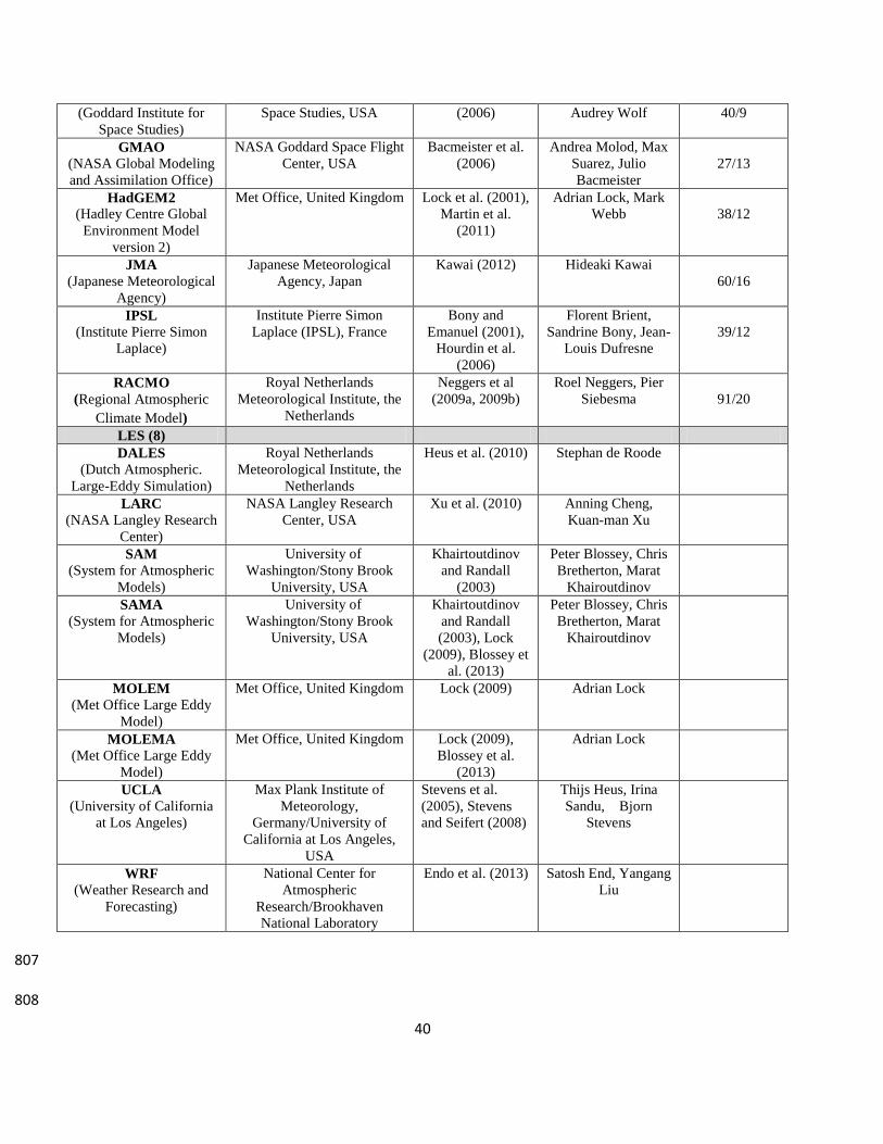
Table 2: Participating models and contributors 804

Table 2: Participating models, main references, and contributors. The number of vertical layers and 805

layers between the surface and 700 hPa for SCMs are given in the last column 806

Models

Acronyms

Model Institution References Contributors Layers: Total/

(p>700 hPa)

SCM (15)

ACCESS

(Australian Community

Climate and Earth System

Simulator)

Australian Commonwealth

Scientific and Industrial

Research

Organisation/Centre for

Australian Weather and

Climate Research

Hewitt et al.

(2011)

Charmaine Franklin

38/12

CAM4

(Community Atmospheric

Model Version 4)

National Center for

Atmospheric Research

(NCAR), USA

Neale et al. (2013) Minghua Zhang,

Cecile Hannay,

Philip Rasch

26/5

CAM5

(Community Atmospheric

Model Version 4)

National Center for

Atmospheric Research

(NCAR), USA

Rasch et al. (2012) Minghua Zhang,

Cecile Hannay,

Philip Rasch

30/9

CCC

(Canadian Centre for

Climate)

Canadian Centre for Climate

Modelling and Analysis,

Canada Ma et al. (2010) Phillip Austin, Knut

von Salzen

35/14

CLUBB

(Cloud Layers Unified By

Binormals)

University of Wisconsin at

Milwaukee, USA

Golaz et al.

(2002a,b),

Larson and Golaz

(2005), Golaz et

al. (2007)

Vincent Larson,

Ryan Senkbeil

41/29

ECHAM6

(ECMWF-University of

Hamburg Model Version

6)

Max-Planck Institute of

Meteorology, Germany

Roeckner et al.

(2011), Stevens et

al.(2013)

Suvarchal Cheedela,

Bjorn Stevens

31/9

ECMWF

(European Center for

Medium Range Weather

Forecasting)

European Center for Medium

Range Weather Forecasting

Neggers et al

(2009a, 2009b)

Martin Koehler

91/20

EC-ETH

(ECMWF-

Eidgenössische

Technische Hochschule)

Swiss Federal Institute of

Technology, Switzerland

Isotta et al. (2011) Colombe

Siegenthaler-Le

Drian, Isotta

Alessandro

Francesco ,Ulrike

Lohman

31/9

GFDL-AM3

(Geophysical Fluid

Dynamics Laboratory

Atmospheric Model

Version 3)

NOAA Geophysical Fluid

Dynamics Laboratory, USA

Donner et al.

(2011)

Jean-Christophe

Golaz, Ming Zhao

48/12

GISS NASA Goddard Institute for Schmidt et al. Anthony DelGenio,

40

(Goddard Institute for

Space Studies)

Space Studies, USA (2006) Audrey Wolf 40/9

GMAO

(NASA Global Modeling

and Assimilation Office)

NASA Goddard Space Flight

Center, USA

Bacmeister et al.

(2006)

Andrea Molod, Max

Suarez, Julio

Bacmeister

27/13

HadGEM2

(Hadley Centre Global

Environment Model

version 2)

Met Office, United Kingdom Lock et al. (2001),

Martin et al.

(2011)

Adrian Lock, Mark

Webb

38/12

JMA

(Japanese Meteorological

Agency)

Japanese Meteorological

Agency, Japan

Kawai (2012) Hideaki Kawai

60/16

IPSL

(Institute Pierre Simon

Laplace)

Institute Pierre Simon

Laplace (IPSL), France

Bony and

Emanuel (2001),

Hourdin et al.

(2006)

Florent Brient,

Sandrine Bony, Jean-

Louis Dufresne

39/12

RACMO

(Regional Atmospheric

Climate Model)

Royal Netherlands

Meteorological Institute, the

Netherlands

Neggers et al

(2009a, 2009b)

Roel Neggers, Pier

Siebesma

91/20

LES (8)

DALES

(Dutch Atmospheric.

Large-Eddy Simulation)

Royal Netherlands

Meteorological Institute, the

Netherlands

Heus et al. (2010) Stephan de Roode

LARC

(NASA Langley Research

Center)

NASA Langley Research

Center, USA

Xu et al. (2010) Anning Cheng,

Kuan-man Xu

SAM

(System for Atmospheric

Models)

University of

Washington/Stony Brook

University, USA

Khairtoutdinov

and Randall

(2003)

Peter Blossey, Chris

Bretherton, Marat

Khairoutdinov

SAMA

(System for Atmospheric

Models)

University of

Washington/Stony Brook

University, USA

Khairtoutdinov

and Randall

(2003), Lock

(2009), Blossey et

al. (2013)

Peter Blossey, Chris

Bretherton, Marat

Khairoutdinov

MOLEM

(Met Office Large Eddy

Model)

Met Office, United Kingdom Lock (2009) Adrian Lock

MOLEMA

(Met Office Large Eddy

Model)

Met Office, United Kingdom Lock (2009),

Blossey et al.

(2013)

Adrian Lock

UCLA

(University of California

at Los Angeles)

Max Plank Institute of

Meteorology,

Germany/University of

California at Los Angeles,

USA

Stevens et al.

(2005), Stevens

and Seifert (2008)

Thijs Heus, Irina

Sandu, Bjorn

Stevens

WRF

(Weather Research and

Forecasting)

National Center for

Atmospheric

Research/Brookhaven

National Laboratory

Endo et al. (2013) Satosh End, Yangang

Liu

807

808

41

809

Table 3: Boundary-layer turbulence schemes in SCMs 810

Models

References Local Kc Cloud-top

entrainment

Counter

Gradient c

ACCESS

Lock et al. (2000) N

Y Y

CAM4

Holtslag and Boville (1993) N N Y

CAM5

Bretherton & Park (2009) Y Y N

CCC

von Salzen et al. (2012) Y Y Y

CLUBB

Golaz et al. (2002a,b),

Larson and Golaz (2005),

Golaz et al. (2007)

Y N N

ECHAM6

Roeckner et al. (2011),

Stevens et al.(2012) Y N N

ECMWF

Neggers et al (2009a,

2009b), Lock (2000) N Y Y

EC-ETH

Brinkop and Roeckner

(1995) Y N N

GFDL-AM3 Lock(2000)

N Y Y

GISS

Holtslag and Moeng (1991)

N Y Y

GMAO

Lock et al. (2000), Louis

(1979) N Y Y

HadGEM2 Lock et al. (2000) N Y Y

JMA

Kawai (2012) Y N N

IPSL

Loius (1992), Houdrin

(2006)

Y N Y

RACMO

Neggers et al (2009a,

2009b) N Y Y

811

812

42

Table 4: Shallow convection schemes. Some models use the same schemes for deep convections 813

Models

Acronyms

References Trigger Lateral

entrainment

Lateral

detrainment

closure

ACCESS

Gregory and Rowntree

(1990), Grant (2001)

undiluted

parcel

specified

specified TKE

CAM4

Hack (1994) undiluted

parcel

N N CAPE

CAM5

Park and Bretherton (2009) CIN+TKE buoyancy

sorting

buoyancy

sorting

CIN+TKE

CCC

von Salzen et al. (2012)

von Salzen and McFarlane

(2002), Grant (2001)

undiluted

parcel

buoyancy

profile

buoyancy

profile

CIN+TKE

CLUBB

Golaz et al. (2002a,b),

Larson and Golaz (2005),

Golaz et al. (2007)

N N N high-order

bi-normal

distribution

ECHAM6

Tidietke (1989)

diluted

parcel

specified specified Large-scale

mass flux

ECMWF

Tidietke (1989) diluted

parcel

specified diagnosed sub-cloud

moist static

energy

EC-ETH

Von Salzen and McFarlane

(2002), Grant (2001)

undiluted buoyancy

profile

buoyancy

profile

TKE

GFDL-AM3 Bretherton & Park (2009) CIN+TKE buoyancy

sorting

buoyancy

sorting

CIN+TKE

GISS

Del Genio and Yao (1993) undiluted

parcel

specified

N CAPE

GMAO

Moorthi and Suarez (1992) undiluted Diagnosed N CAPE

HadGEM2 Gregory and Rowntree

(1990), Grant (2001)

undiluted

parcel

specified

specified TKE

JMA

Kawai (2012) diluted

parcel

diagnosed N prognostic

IPSL

Emanuel (1991) undiluted

parcel

buoyancy

sorting

buoyancy

sorting

CAPE

RACMO

Neggers et al (2009a,

2009b)

unified with

PBL scheme

unified with

PBL scheme

unified with

PBL scheme

unified with

PBL

scheme

814

815

43

Figure Captions 816

Figure 1: Schematics of the experimental setup. The atmospheric temperature and water vapor 817

are constructed based on moist adiabat and fixed relative humidity respectively. The large-scale 818

subsidence is calculated based on the clear-sky thermodynamic equation. These fields change with 819

SST, which is given warming of 2oC in the perturbed climate. 820

Figure 2: Averaged amount of low clouds in June-July-August (%) from the C3M satellite data. 821

The red line is the northern portion of the GPCI (see text); the symbols “S6”, “S11” and “S12” are the 822

three locations studied in the paper. 823

Figure 3: (a) Large-scale pressure vertical velocity at the three locations in the control climate 824

(solid lines), and in the ERA-Interim (dashed). (b) Same as (a) except that the dashed lines denote 825

subsidence rates in the warmer climate. (c) Same as (b) except for horizontal advective tendency of 826

temperature. (d) Same as (c) except for advective tendency of water vapor. 827

Figure 4: (a)-(c) are the averaged profiles of cloud amount (%) by SCMs for S6, S11 and S12 828

respectively (from top to bottom panels). (d)-(f) are the same as (a)-(c) but by the LES models. (g)-(i) 829

are from the C3M satellite measurements. The blue lines are ensemble averages; the red lines are the 830

25% and 75% percentiles. 831

Figure 5: Examples of time evolution of cloud amount (%) simulated by JMA (left column) for 832

S6, S11 and S12 respectively from top to bottom panels; CAM4 (middle column); GISS (third 833

column) ; SAMA (right column). 834

835

44

Figure 6: Examples of physical tendencies (g/kg/day) of water vapor budget in three SCMs at 836

S11 for the control climate, “turb” for turbulence scheme, “conv” for convection scheme, “(c-e)” for 837

net large-scale condensation. The dashed lines are cloud liquid water (0.1g/kg). The black dots show 838

the mid-point of model layers. (a) JMA, (b) CAM4, (c) GISS. 839

Figure 7: (a) Change of cloud radiative forcing (CRF, W/m2) in SCMs at location S11 840

corresponding to 2oK SST perturbation. Character “X” above a model’s name indicates that the 841

shallow convection scheme is not active; “O” indicates that the shallow convection scheme is active. 842

Models without these characters either do not separately parameterize shallow convection and PBL 843

turbulence, or do not submit results with convection information. 844

Figure 8: (a) Change of moisture tendency in the layer of maximum cloud water (g/kg/day) by 845

the “Turb” term from the control climate to the perturbed climate at S11. (b) Same as (a) but for 846

surface latent heat flux (W/m2). 847

Figure 9: Schematics of cloud feedbacks. Changes of clouds from the control (left) to warmer 848

(right) climates. Blue arrows denote the term of turbulence parameterization in the moisture budget 849

equation; red arrows denote shallow convection; black arrows denote cloud-top entrainment, lateral 850

mixing and dry tiubulence. The sizes of arrows schematically correspond to the magnitude of moisture 851

tendency from the associated processes. (a) Negative cloud feedback, dominated by the increase of 852

surface turbulence. (b) Positive cloud feedback, dominated by the increase of shallow convection or 853

cloud-top entrainment. (c) Cloud feedback from shallow cumulus with sufficient depth, with sign 854

depending on the cloud depth and lateral mixing. 855

45

Figure 10: Same as Figure 7, but for (a) S6, (b) S12. The models are ordered in the same 856

sequence as in Figure 7. One model (EC_ECH) did not reach quasi-equilibrium state and it is indicated 857

by “N/A”. 858

Figure 11: Same as Figure 7 but in LES models. (a) S6; (b) S11; (c) S12. 859

860

861

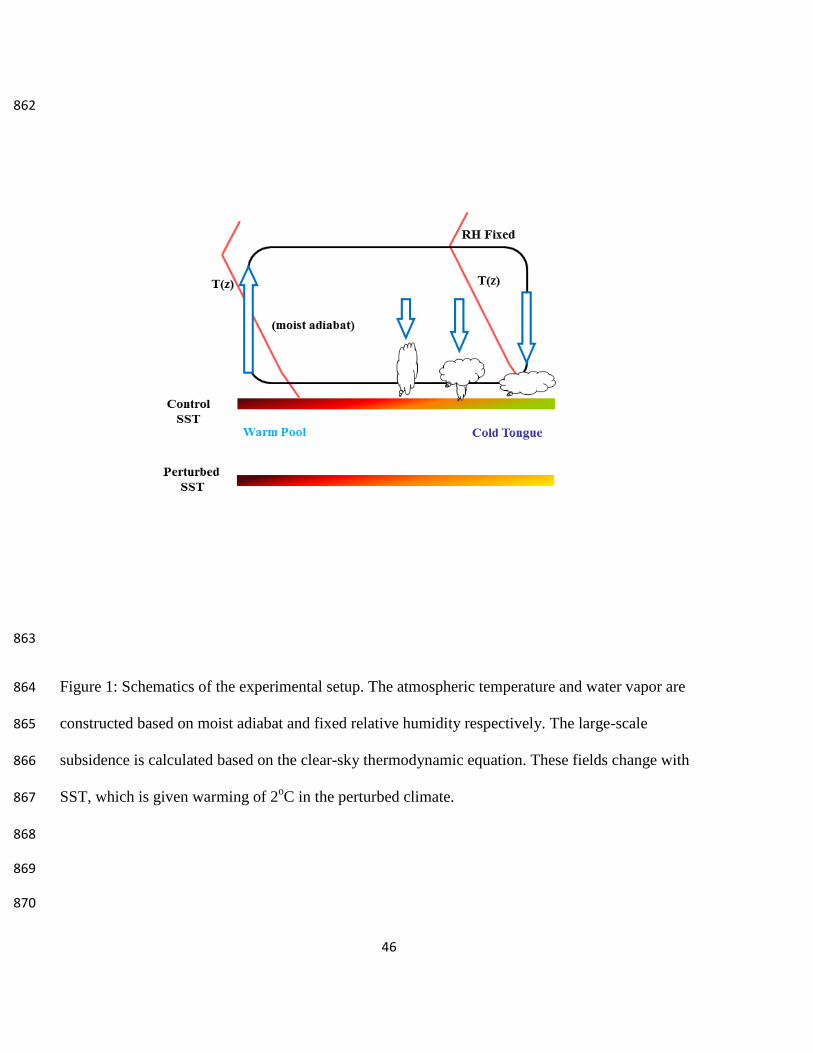
46

862

863

Figure 1: Schematics of the experimental setup. The atmospheric temperature and water vapor are 864

constructed based on moist adiabat and fixed relative humidity respectively. The large-scale 865

subsidence is calculated based on the clear-sky thermodynamic equation. These fields change with 866

SST, which is given warming of 2oC in the perturbed climate. 867

868

869

870

47

871

872

Figure 2: Averaged amount of low clouds in June-July-August (%) from the C3M satellite data. The 873

red line is the northern portion of the GPCI (see text); the symbols “S6”, “S11” and “S12” are the 874

three locations studied in the paper. 875

876

877

878

879

48

880 881

Figure 3: (a) Large-scale pressure vertical velocity (subsidence) at the three locations in the control 882

climate (solid lines), and in the ERA-Interim (dashed lines). (b) Same as (a) except that the dashed 883

lines denote subsidence rates in the warmer climate. (c) Same as (b) except for horizontal advective 884

tendency of temperature. (d) Same as (b) except for horizontal advective tendency of water vapor. 885

886

49

887

Figure 4: (a)-(c) are the averaged profiles of cloud amount (%) by SCMs for S6, S11 and S12 888

respectively (from top to bottom panels). (d)-(f) are the same as (a)-(c) but by the LES models. (g)-(i) 889

are from the C3M satellite measurements. The blue lines are ensemble averages; the red lines are the 890

25% and 75% percentiles. 891

892

893

50

894

Figure 5: Examples of time evolution of cloud amount (%) simulated by JMA (left column) for S6, 895

S11 and S12 respectively from top to bottom panels; CAM4 (middle column); GISS (third column) ; 896

SAMA (right column). 897

898

899

900

901

51

902

903

Figure 6: Examples of physical tendencies (g/kg/day) of water vapor budget in three SCMs at S11 for 904

the control climate, “turb” for turbulence scheme, “conv” for convection scheme, “(c-e)” for net large-905

scale condensation. The dashed lines are cloud liquid water (0.1g/kg). The black dots show the mid-906

point of model layers. (a) JMA, (b) CAM4, (c) GISS. 907

908

909

52

910

Figure 7: (a) Change of cloud radiative forcing (CRF, W/m2) in SCMs at location S11 corresponding 911

to 2oK SST perturbation. Character “X” above a model’s name indicates that the shallow convection 912

scheme is not active; “O” indicates that the shallow convection scheme is active. Models without these 913

characters either do not separately parameterize shallow convection and PBL turbulence, or do not 914

submit results with convection information. 915

916

917

53

918

Figure 8: (a) Change of moisture tendency in the layer of maximum cloud water (g/kg/day) by the 919

“Turb” term from the control climate to the perturbed climate at S11. (b) Same as (a) but for surface 920

latent heat flux (W/m2). 921

922

923

924

54

925

926

Figure 9: Schematics of cloud feedbacks. Changes of clouds from the control (left) to warmer (right) 927

climates. Blue arrows denote the term of turbulence parameterization in the moisture budget equation; 928

red arrows denote shallow convection; black arrows denote cloud-top entrainment, lateral mixing and 929

dry tiubulence. The sizes of arrows schematically correspond to the magnitude of moisture tendency 930

from the associated processes. (a) Negative cloud feedback, dominated by the increase of surface 931

turbulence. (b) Positive cloud feedback, dominated by the increase of shallow convection or cloud-932

top entrainment. (c) Cloud feedback from shallow cumulus with sufficient depth, with sign depending 933

on the cloud depth and lateral mixing. 934

55

935

936

937

Figure 10: Same as Figure 7, but for (a) S6, (b) S12. The models are ordered in the same sequence as 938

in Figure 7. One model (EC_ECH) did not reach quasi-equilibrium state and it is indicated by “N/A”. 939

940

56

941

942

Figure 11: Same as Figure 7 but in LES models. (a) S6; (b) S11; (c) S12. 943

944