1 case study i: parallel molecular dynamics and namd: laxmikant kale parallel programming...
TRANSCRIPT

1
Case Study I:Parallel Molecular Dynamics and
NAMD: Laxmikant Kale
http://charm.cs.uiuc.eduParallel Programming Laboratory
University of Illinois at Urbana Champaign

3
NAMD: A Production MD program
NAMD
• Fully featured program
• NIH-funded development
• Distributed free of charge (~5000 downloads so far)
• Binaries and source code
• Installed at NSF centers
• User training and support
• Large published simulations (e.g., aquaporin simulation featured in keynote)

4
NAMD, CHARMM27, PMENpT ensemble at 310 or 298 K 1ns equilibration, 4ns production
Protein:~ 15,000 atomsLipids (POPE): ~ 40,000 atomsWater: ~ 51,000 atomsTotal: ~ 106,000 atoms
3.5 days / ns - 128 O2000 CPUs11 days / ns - 32 Linux CPUs.35 days/ns–512 LeMieux CPUs
Acquaporin Simulation
F. Zhu, E.T., K. Schulten, FEBS Lett. 504, 212 (2001)M. Jensen, E.T., K. Schulten, Structure 9, 1083 (2001)

5
Molecular Dynamics in NAMD
• Collection of [charged] atoms, with bonds– Newtonian mechanics
– Thousands of atoms (10,000 - 500,000)
• At each time-step– Calculate forces on each atom
• Bonds:
• Non-bonded: electrostatic and van der Waal’s– Short-distance: every timestep
– Long-distance: using PME (3D FFT)
– Multiple Time Stepping : PME every 4 timesteps
– Calculate velocities and advance positions
• Challenge: femtosecond time-step, millions needed!
Collaboration with K. Schulten, R. Skeel, and coworkers

6
Sizes of Simulations Over Time
BPTI3K atoms
Estrogen Receptor36K atoms (1996)
ATP Synthase327K atoms
(2001)
7
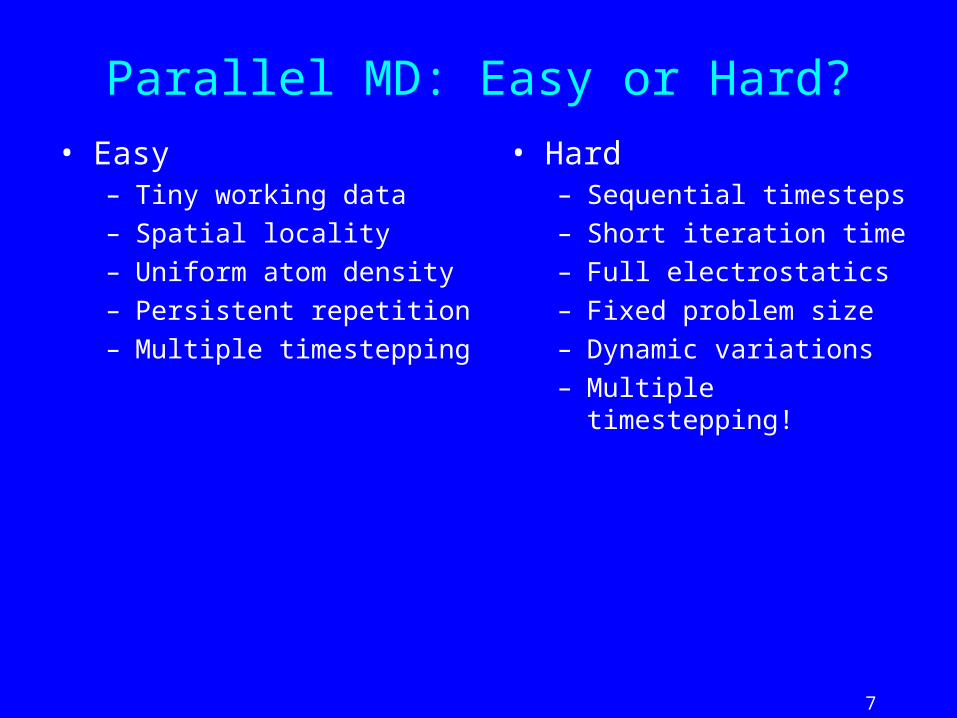
Parallel MD: Easy or Hard?
• Easy– Tiny working data
– Spatial locality
– Uniform atom density
– Persistent repetition
– Multiple timestepping
• Hard– Sequential timesteps
– Short iteration time
– Full electrostatics
– Fixed problem size
– Dynamic variations
– Multiple timestepping!

8
Other MD Programs for Biomolecules
• CHARMM• Amber• GROMACS• NWChem• LAMMPS

9
Traditional Approaches: non isoefficient
• Replicated Data:– All atom coordinates stored on each processor
• Communication/Computation ratio: P log P
• Partition the Atoms array across processors– Nearby atoms may not be on the same processor
– C/C ratio: O(P)
• Distribute force matrix to processors– Matrix is sparse, non uniform,
– C/C Ratio: sqrt(P)

10
Spatial Decomposition
•Atoms distributed to cubes based on their location
• Size of each cube :
•Just a bit larger than cut-off radius
•Communicate only with neighbors
•Work: for each pair of nbr objects
•C/C ratio: O(1)
•However:
•Load Imbalance
•Limited Parallelism
Cells, Cubes or“Patches”
Charm++ is useful to handle this

11
Virtualization: Object-based Parallelization
User View
System implementation
User is only concerned with interaction between objects

12
Data driven execution
Scheduler Scheduler
Message Q Message Q
13
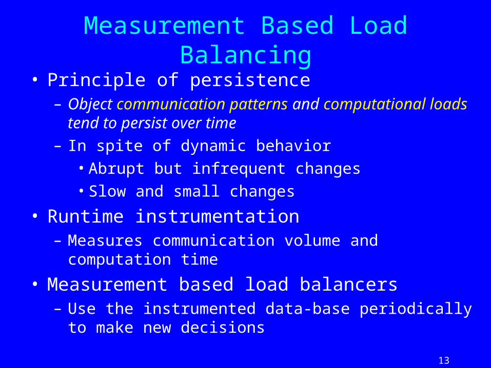
Measurement Based Load Balancing
• Principle of persistence– Object communication patterns and computational loads
tend to persist over time
– In spite of dynamic behavior
• Abrupt but infrequent changes
• Slow and small changes
• Runtime instrumentation– Measures communication volume and computation time
• Measurement based load balancers– Use the instrumented data-base periodically to make new
decisions
14
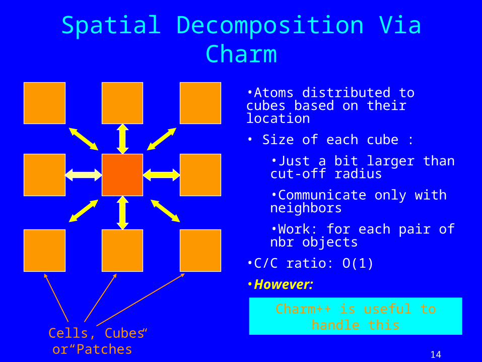
Spatial Decomposition Via Charm
•Atoms distributed to cubes based on their location
• Size of each cube :
•Just a bit larger than cut-off radius
•Communicate only with neighbors
•Work: for each pair of nbr objects
•C/C ratio: O(1)
•However:
•Load Imbalance
•Limited Parallelism
Cells, Cubes or“Patches”
Charm++ is useful to handle this

15
Object Based Parallelization for MD:
Force Decomposition + Spatial Decomposition
•Now, we have many objects to load balance:
–Each diamond can be assigned to any proc.
– Number of diamonds (3D):
–14·Number of Patches
17
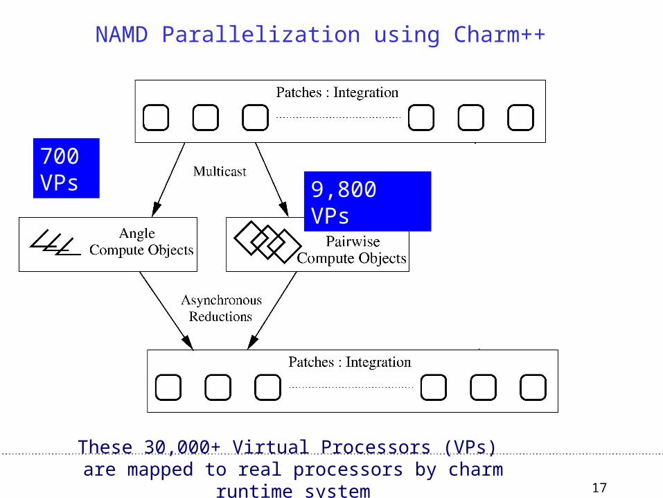
700 VPs
NAMD Parallelization using Charm++
These 30,000+ Virtual Processors (VPs) are mapped to real processors by charm runtime system
9,800 VPs

18
Optimizing multicast

19

20
128 processors: utilization and load balancing

21
1024 procs

22

23

24

25

26

27

28

29
Performance Data: SC2000
Speedup on Asci Red
0
200
400
600
800
1000
1200
1400
0 500 1000 1500 2000 2500
Processors
Sp
eed
up

30
New Challenges
• New parallel machine with faster processors– PSC Lemieux
– 1 processor performance:
• 57 seconds on ASCI red to 7.08 seconds on Lemieux
– Makes is harder to parallelize:
• E.g. larger communication-to-computation ratio
• Each timestep is few milliseconds on 1000’s of processors
• Incorporation of Particle Mesh Ewald (PME)
31
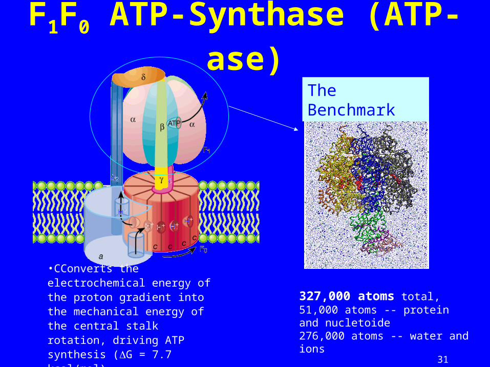
F1F0 ATP-Synthase (ATP-ase)
•CConverts the electrochemical energy of the proton gradient into the mechanical energy of the central stalk rotation, driving ATP synthesis (G = 7.7 kcal/mol).
327,000 atoms total,51,000 atoms -- protein and nucletoide276,000 atoms -- water and ions
The Benchmark

33
Grainsize and Amdahls’s law
• A variant of Amdahl’s law, for objects:– The fastest time can be no shorter than the time for the
biggest single object!
– Lesson from previous efforts
• Splitting computation objects:– 30,000 nonbonded compute objects
– Instead of approx 10,000
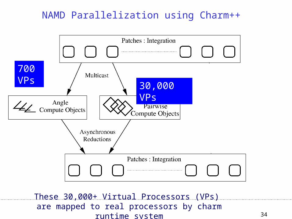
34
700 VPs
NAMD Parallelization using Charm++
These 30,000+ Virtual Processors (VPs) are mapped to real processors by charm runtime system
30,000 VPs

35
Mode: 700 us
Distribution of execution times of
non-bonded force computation objects (over 24 steps)

37
Load Balancing Steps
Regular Timesteps
Instrumented Timesteps
Detailed, aggressive Load Balancing
Refinement Load Balancing

38
Another New Challenge
• Jitter due small variations– On 2k processors or more
– Each timestep, ideally, will be about 12-14 msec for ATPase
– Within that time: each processor sends and receives :
• Approximately 60-70 messages of 4-6 KB each
– Communication layer and/or OS has small “hiccups”
• No problem until 512 processors
• Small rare hiccups can lead to large performance impact– When timestep is small (10-20 msec), AND
– Large number of processors are used

39
Benefits of Avoiding Barrier• Problem with barriers:
– Not the direct cost of the operation itself as much
– But it prevents the program from adjusting to small variations
• E.g. K phases, separated by barriers (or scalar reductions)
• Load is effectively balanced. But,– In each phase, there may be slight non-determistic load imbalance
– Let Li,j be the load on I’th processor in j’th phase.
• In NAMD, using Charm++’s message-driven execution:– The energy reductions were made asynchronous
– No other global barriers are used in cut-off simulations
k
jjii L
1, }{max }{max
1,
k
jjii LWith barrier: Without:

40
100 milliseconds

41
Substep Dynamic Load Adjustments
• Load balancer tells each processor its expected (predicted) load for each timestep
• Each processor monitors its execution time for each timestep – after executing each force-computation object
• If it has taken well beyond its allocated time:– Infers that it has encountered a “stretch”
– Sends a fraction of its work in the next 2-3 steps to other processors
• Randomly selected from among the least loaded processors
migrate Compute(s) away in this step

42
NAMD on Lemieux without PMEProcs Per Node Time (ms) Speedup GFLOPS
1 1 24890 1 0.494
128 4 207.4 119 59
256 4 105.5 236 116
512 4 55.4 448 221
510 3 54.8 454 224
1024 4 33.4 745 368
1023 3 29.8 835 412
1536 3 21.2 1175 580
1800 3 18.6 1340 661
2250 3 14.4 1728 850
ATPase: 327,000+ atoms including water

43
Adding PME
• PME involves:– A grid of modest size (e.g. 192x144x144)
– Need to distribute charge from patches to grids
– 3D FFT over the grid
• Strategy:– Use a smaller subset (non-dedicated) of processors for PME
– Overlap PME with cutoff computation
– Use individual processors for both PME and cutoff computations
– Multiple timestepping

44
700 VPs
192 + 144 VPs
30,000 VPs
NAMD Parallelization using Charm++ : PME
These 30,000+ Virtual Processors (VPs) are mapped to real processors by charm runtime system

45
Optimizing PME
• Initially, we used FFTW for parallel 3D FFT– FFTW is very fast, optimizes by analyzing machine and FFT
size, and creates a “plan”.
– However, parallel FFTW was unsuitable for us:
• FFTW not optimize for “small” FFTs needed here
• Optimizes for memory, which is unnecessary here.
• Solution:– Used FFTW only sequentially (2D and 1D)
– Charm++ based parallel transpose
– Allows overlapping with other useful computation

46
Communication Pattern in PME
192
procs
144 procs

47
Optimizing Transpose
• Transpose can be done using MPI all-to-all– But: costly
• Direct point-to-point messages were faster
– Per message cost significantly larger compared with total per-byte cost (600-800 byte messages)
• Solution:– Mesh-based all-to-all
– Organized destination processors in a virtual 2D grid
– Message from (x1,y1) to (x2,y2) goes via (x1,y2)
– 2.sqrt(P) messages instead of P-1.
– For us: 28 messages instead of 192.

48
All to all via MeshOrganize processors in a 2D (virtual) grid
Phase 1:
Each processor sends messages within its row
Phase 2:
Each processor sends messages within its column
Message from (x1,y1) to (x2,y2) goes via (x1,y2)
2. messages instead of P-1 1P
For us: 26 messages instead of 192
1P
1P

50
Impact on Namd Performance
0
20
40
60
80
100
120
140
Step Time
256 512 1024
Processors
MeshDirectMPI
Namd Performance on Lemieux, with the transpose step implemented using different all-to-all algorithms

52
Performance: NAMD on Lemieux
Time (ms) Speedup GFLOPSProcs Per Node Cut PME MTS Cut PME MTS Cut PME MTS
1 1 24890 29490 28080 1 1 1 0.494 0.434 0.48128 4 207.4 249.3 234.6 119 118 119 59 51 57256 4 105.5 135.5 121.9 236 217 230 116 94 110512 4 55.4 72.9 63.8 448 404 440 221 175 211510 3 54.8 69.5 63 454 424 445 224 184 213
1024 4 33.4 45.1 36.1 745 653 778 368 283 3731023 3 29.8 38.7 33.9 835 762 829 412 331 3971536 3 21.2 28.2 24.7 1175 1047 1137 580 454 5451800 3 18.6 25.8 22.3 1340 1141 1261 661 495 6052250 3 14.4 23.5 17.54 1728 1256 1601 850 545 770
ATPase: 320,000+ atoms including water

53
200 milliseconds

54
Using all 4 processors on each Node
300 milliseconds

55
Conclusion
• We have been able to effectively parallelize MD, – A challenging application
– On realistic Benchmarks
– To 2250 processors, 850 GF, and 14.4 msec timestep
– To 2250 processors, 770 GF, 17.5 msec timestep with PME and multiple timestepping
• These constitute unprecedented performance for MD– 20-fold improvement over our results 2 years ago
– Substantially above other production-quality MD codes for biomolecules
• Using Charm++’s runtime optimizations• Automatic load balancing
• Automatic overlap of communication/computation– Even across modules: PME and non-bonded
• Communication libraries: automatic optimization