These notes are prepared by: A.R. Hajiaboli

1. Basics of Quantum Mechanics 1.1 Energy quantization One of the basic differences between classical mechanics and its quantum counterpart is that whereas classical mechanics allows particles in a system to have any energy within a given limit, quantum mechanics postulates that a particle can only have a particular set of discrete allowed energy, meeting certain constraints. When a particle jumps from one discrete state to another, it either absorbs or emits energy quanta (most frequently it is photon) which corresponds to a particular wavelength associated with the difference of the two states’ energy, given by:

υhE = , Where h is the Plank’s constant and ν is the frequency. Generally, if the system is quite large (regarding quantum scale), the difference in energy quantization is very small and a smooth continuous energy can be approximated (as in the case of bulk semiconductor where we assume that conduction and valence electrons form bands which are continuous in their given energy range). But if the system is small enough, the difference between quantized energy states become significant. Thin films are a good example, in which if the thickness is in nanoscale, then energy of electrons in that direction becomes quantized and effectively confined, and we obtain the so called 2 Dimensional Electron Gas. This was first demonstrated in 1900, when Max Plank in his experiments with blackbody radiation found out that the existing wave mechanics for heat radiation predicts that intensity of radiation should follow:

41λ∝I

Which is true for large wavelengths but fails for shorter wavelengths where the experimental result deviates from the theory drastically.

The only way to explain is to think the radiation to be discrete particle like, which he called ‘Quanta’ and follow the equation:

υnhE = , With n being an integer.

erhaps a more interesting example of this could be that of the photoelectric effect, at Pleast from the electrical engineering viewpoint, which was explained by Einstein in 1905 with application of Plank’s theory to light and for the first time introducing the terminology ‘Photon’ as the quanta of light. In this effect light is shone on a metal, and electrons are released. These electrons can be attracted towards a positively charged plate a certain distance below, thereby establishing a photoelectric current.

is convenient not to measure this current itself but to measure the stopping potential V0 Itrequired to reduce this current to zero. The stopping potential is related to the (maximum) kinetic energy of the ejected electrons by

2max2

1max0 ..EKeV = mv=

here were several failings of the wave picture of light when applied to this phenomenon, Tbut the most notable was that no photoelectrons are emitted if the frequency of the light falls below some cutoff frequency, fc. This aspect of the photoelectric effect is impossible to understand within the wave picture of light, as within that picture the energy of the light beam which gives the electrons their energy does not depend on the frequency. Einstein came up with an explanation of the photoelectric effect which built upon Planck's photon hypothesis. In this theory Einstein assumed that photons have energy equal to the energy difference between adjacent levels of a blackbody:

υhE =

When these photons hit the metal, they could give up some or all of their energy to an electron. A certain amount of energy would be required to release the electrons from their bonds to the metal - this energy is called the work function, Ф, of the metal. The remaining energy would appear as kinetic energy of the released electron. Thus, the maximum kinetic energy the electrons could have is

Φ−=Φ−==λ

υ hchEKeV .. max0

Thus, stopping potential V0 vs. frequency f is a straight line, with slope related to Planck's constant h and x-intercept being the cutoff frequency, fc where V = 0 : 0

λc

hfc =

Φ=

here λc is the corresponding cutoff wavelength. This behavior is observed

.2 Wave particle duality

previous section it is seen that in some experiments, light acts as particle rather than

Wexperimentally, and the success of this explanation made more and more people take the photon picture of light seriously. 1 Inwave. But there are other experiments where light distinctly exhibit such phenomena (e.g. interference and diffraction) that can only be explained if light is considered to be a wave. One important aspect is that in a particular experiment, we can only observe either particle or wave nature of light, but not both. Quantum mechanics appreciates this fact by incorporating wave particle duality for light, and this results in the following equations:

khp h==λ

Here we can see that momentum p, which is a particle property is related to wave vector

1924 a young physicist, de Broglie, speculated that nature did not single out light as

k which is distinctly a wave property. Inbeing the only matter which exhibits a wave-particle duality. He proposed that ordinary “particles” such as electrons, protons, or bowling balls could also exhibit wave characteristics in certain circumstances. Quantitatively, he associated a wavelength to a particle of mass m moving at speed v:

mvh

=λ

ince the momentum of such a particle is p = mv, mathematically this relation is

equivalent to the earlier equation for the momentum of a photon (as found in Compton S

scattering). However, we should emphasize that these two equations have a very different physical content. This wave nature for matter particles is called De Broglie wave and wavelength λ is called De Broglie wavelength for that particle. Relatively straightforward tests of this hypothesis of De Broglie are offered by diffraction and interference - if a beam of such ‘particles’ were shone at a diffraction grating and a

.3 Uncertainty Principle

the wave-particle duality of nature was discovered by eisenberg, and is called ‘The Uncertainty Principle’. To formulate it, let us imagine that

diffraction pattern of a series of light and dark fringes results, then one would be forced to adopt the wave picture for this phenomena. We recall that for a good diffraction pattern to result the size of the diffraction slits should be of the same order as the wavelength of the light used. For macroscopic objects such as bowling balls this would require sizes of slits of the order of 10-34 m or so, which is much outside present-day technology. However, for electrons the sizes of slits required are of the order of 10-11 m or so, which are readily available. In one such experiment by Davisson and Germer in 1927, electrons from a heated filament were accelerated at normal incidence onto a single crystal of nickel and the result showed similar interference patterns to that of light. Therefore, Nature seems to be symmetric, in that light and ordinary ‘particles’ exhibits this wave-particle duality. In fact this is the basis on which we use wave theory to describe the motion and behavior of electrons in a crystal. 1 One important consequence ofHwe want to measure the position and the momentum of a particular particle. To do so we must ‘see’ the particle, and so we shine some light of wavelength on it. We recall that there is a limit to the resolving power of the light used to see the particle given by the wavelength of light used. This gives an uncertainty in the particle's position:

λ≥Δx This results from considering the light as a wave. However, viewed as a photon, the light when striking the particle could give up some or all of its momentum to the particle. Since we do not know how much it gave up, as we do not measure the photon's properties, there is an uncertainty in the momentum of the particle; we find

λhp ≥Δ

Combining these equations, we find

hpx ≥Δ⋅Δ Note that this is independent of the wavelength used, and says there is a limit in principle s to how accurately one can simultaneously measure the position and momentum of a a

particle - if one tries to measure the position more accurately by using light of a shorter wavelength, then the uncertainty in momentum grows, whereas if one uses light of a longer wavelength in order to reduce the uncertainty in momentum, then the uncertainty

in position grows. One cannot reduce both down to zero simultaneously - this is a direct consequence of the wave-particle duality of nature. As with de Broglie waves, for everyday macroscopic objects such as bowling balls the

ncertainty principle plays a negligible role in limiting the accuracy of measurements.

lated two statements in his uncertainty rinciple; the first statement is that it is impossible to simultaneously describe with

uHowever, for microscopic objects such as electrons in atoms the uncertainty principle does become a very important consideration. As history goes, Heisenberg actually postupabsolute accuracy the position and momentum of a particle, as shown above. The second statement is that it is impossible to simultaneously describe with absolute accuracy the energy of a particle and the instant of time the particle has this energy.

htE ≥Δ⋅Δ For a more rigorous formulation, the uncertainty principle states that any two Hermitian

uantum operators which are commutative exhibit this uncertainty of simultaneous

.4 Classical Mechanics vs. Quantum Mechanics

mechanics we can find some teresting difference in predictions made by classical mechanics and quantum

ped within the box could have any energy.

2. the particle should have Brownian motion and has an equal probability of being anywhere and everywhere in the box.

3. tainable

simultaneously for the particle in question.

4. easurable.

x as long as its energy is lower than that of the box.

qmeasurements. 1 Considering the above basic concepts of quantuminmechanics. It should only be relevant to state here the erroneous predictions that classical mechanics arrives at. Suppose we are investigating a system in which we have a very small particle (e.g. an electron) trapped in a 3D box, such that the energy of the particle is less than that of the box. For such a simple system, classical mechanics predicts that:

1. As long as the particle has energy less than that of the box, the particle trap

If no other forces are in the system, then

The exact position and momentum of the particle should be ob

At a particular moment, the exact energy of the particle should be m

5. The particle must be confined in the box and has no chance of escaping the bo

6. If by any chance the particle attains energy larger than that of the box, the particle

ut interestingly quantum mechanics predicts that:

ny energy, and will have only certain

. The particle has certain preferable points, where the probability of finding the

3. We cannot measure the momentum and the position of the particle in the box

4. At an exact moment, the energy is not measurable above a certain extent

5. The particle has a finite chance of escaping the system even with lower energy than

6. If by any chance the particle attains energy larger than that of the box, there remains

is only trivial to state here that in every case, experiments have resulted in favor or

.5 Basic Postulates

ate 1920’s Ervin Schrodinger developed wave mechanics based on Planck’s theory and

proach in terms of matrix algebra called

will certainly leave the box

B1. A particle trapped in such a box cannot have a

allowed energy.

2particle is more than in other parts.

simultaneously without certain uncertainty.

the box.

certain probability that particle might still be trapped inside.

Itquantum mechanics. 1 Lde Broglie’s idea of the wave nature of matter. Warner Heisenberg formulated an alternative apMatrix Mechanics. Postulate I: (in one-dimensional system)

contains all the measurable information about There exists a state function Ψ(x;t) whicheach particle of a physical system. Ψ(x;t) is also called wave function. Postulate II: Every dynamical variable has a corresponding operator. This operator is operated on the

bservables and Operators

or a given system, we are concerned with measuring quantities that are pertinent to us,

state function to obtain measurable information about the system. O Flike as electrical engineers we are concerned with current, capacitance, conductance, carrier density etc. which in spite of the apparently bizarre nature of quantum mechanics,

must remain readily interpretable and obviously real. To account for this, quantum mechanics defines any such parameter which can be measured experimentally and hence has physical significance, to be ‘Observables’ and restrict them to be always real numbers. Then it associates certain operators with every observable and postulates that each operator associated with a particular observable gives the result in real number for that particular observable. It restricts any physical experiments to result in only eigenvalues of that operator. What it effectively states that we can predict the outcome of a physical experiment only by mathematics under the constraint of the above mentioned concepts. Mathematically, quantum mechanic postulates that:

1. Associated with every physical observable is a corresponding operator  from

2. The only result of a measurement on a single system of a physical observable

3. For every system there always exists a state function Ψ that contains all of the

4. The time evolution of the Ψ is determined by

which results of measurement of the observable may be deduced.

associated with the operator  is an eigenvalue of the operator Â.

information that is known about the system.

Ψ=Ψ∂∂ Hi th , where H is the

short list of operators associated with certain observables is given herewith:

Hamiltonian operator for the system.

A

Postulate III: tion Ψ(x;t) and its space derivative ∂Ψ/∂x must be continuous finite and

lized i.e.

onjugate of Ψ. Obviously Ψ Ψ* is a positive and real number and is

le particle-like electron; then Ψ Ψ* is interpreted as the statistical e. Thus

rresponding to the state function Ψ is given by

The state funcsingle-valued for all values of x. The state function must be norma Ψ* is the complex cequal to /Ψ/². Assume a singprobability that the particle is found in a distance element dx at any instant of timΨ Ψ* represents the probability density. The average value ⟨Q⟩ of any variable coexpectation value:

dxQQ ΨΨ=∧∞

∞−

∗∫

lue of many observations.

icle was found, it was possible to

2.1 ave function

has been established that every particle has a wave nature associated with it. In

general, this wave function is a function of time and space, and can be complex in

⟨Q⟩ is the expected vaOnce the state function corresponding to any partcalculate the average position, energy and momentum of the particle within the limit of the uncertainty principle. 2. Schrödinger’s Equation

W

Itquantum mechanics it is customary to associate with every particle a wave function, ψ to account for that wave nature. This wave function contains all and every information about the particle. It is usually found as the solution to Schrödinger’s equation corresponding to a particular system. To extract meaningful information from it, one must use the appropriate operators on it for the parameter in concern. Innature. In itself, it has no physical significance, but the squared magnitude of it gives the probability density of a particle. Since (in most representation of quantum mechanics, but not all) it has to be found as the solution of Schrödinger’s equation, some constraints are imposed on it.

1. Normalization: The squared magnitude gives the probability density of finding the particle. So if we are talking about one single particle, it must be there in the universe, so the squared magnitude of the wave function should equal to 1. this is stated mathematically as:

( ) ( ) 1,, 3* =∫ rdtrtr ψψ 2. Function must be finite, continuous and single valued. It is only obvious that if a

wave function is not continuous, then its squared magnitude cannot predict the probability at that point of discontinuity and a multi-valued wave function would result in ambiguous probability.

3. The first derivative must also be finite, continuous and single valued. This results

also from the mathematical considerations. 2.2 Time independent Schrödinger’s equation We start with the one-dimensional classical wave equation,

By introducing the separation of variables

we obtain

If we introduce one of the standard wave equation solutions for f(t) such as (the constant can be taken care of later in the normalization), we obtain

Now we have an ordinary differential equation describing the spatial amplitude of the matter wave as a function of position. The energy of a particle is the sum of kinetic and potential parts

which can be solved for the momentum, p, to obtain

Now we can use the de Broglie formula to get an expression for the wavelength

2 2/υ in equation can be rewritten in terms of λ if we recall that The term ω and .

When this result is substituted into equation we obtain the famous time-independent Schrödinger equation

which is almost always written in the form

This single-particle one-dimensional equation can easily be extended to the case of three dimensions, where it becomes

A two-body problem can also be treated by this equation if the mass m is replaced with a reduced mass µ. It is important to point out that this analogy with the classical wave equation only goes so far. We cannot, for instance, derive the time-dependent Schrödinger equation in an analogous fashion (for instance, that equation involves the partial first derivative with respect to time instead of the partial second derivative). In fact, Schrödinger presented his time-independent equation first, and then went back and postulated the more general time-dependent equation. 2.3 Time dependant Schrödinger’s Equation Although we were able to derive the single-particle time-independent Schrödinger equation starting from the classical wave equation and the de Broglie relation, the time-

dependent Schrödinger equation cannot be derived using elementary methods and is generally given as a postulate of quantum mechanics. It is possible to show that the time-dependent equation is at least reasonable if not derivable, but the arguments are rather involved. The single-particle three-dimensional time-dependent Schrödinger equation is

Where V is assumed to be a real function and represents the potential energy of the system (a complex function V will act as a source or sink for probability). Wave Mechanics is the branch of quantum mechanics with this equation as its dynamical law. Note that this equation does not yet account for spin or relativistic effects. Of course the time-dependent equation can be used to derive the time-independent equation. If we write the wavefunction as a product of spatial and temporal terms,

, then equation becomes

or

Since the left-hand side is a function of t only and the right hand side is a function of only, the two sides must equal a constant. If we tentatively designate this constant E (since the right-hand side clearly must have the dimensions of energy), then we extract two ordinary differential equations, namely

and

The latter equation is once again the time-independent Schrödinger equation. The former equation is easily solved to yield

The Hamiltonian in this equation is a Hermitian operator, and the eigenvalues of a Hermitian operator must be real, so E is real. This means that the solutions f(t) are purely oscillatory, since f(t) never changes in magnitude Thus if

then the total wave function differs from only by a phase factor of constant magnitude. There are some interesting consequences of this. First of all, the

quantity is time independent, as we can easily show:

Secondly, the expectation value for any time-independent operator is also time-independent, if satisfies equation. By the same reasoning applied above,

For these reasons, wave functions of the form are called stationary states. The state

is ‘stationary’, but the particle it describes is not! Of course equation represents a particular solution to equation. The general solution to equation will be a linear combination of these particular solutions, i.e.

2.4 plane wave Schrödinger’s equation can be used to find the wavefunction of an electron which is free from any confining potential. This could be a truly free electron, or an apparently free electron in the conduction band with an effective mass associated with it. If there is no force acting on the particle, then the potential function V(r) will be constant and we must have E>V(r). Let us assume for simplicity that V(r)=0 for all values, and consider only 1D case so that r ≡ x. Then the time independent wave equation can be written as:

( ) ( ) 0222

2

=+∂

∂ xmEx

x ψψh

The solution to this differential equation can be written as:

( ) ( ) ( )hh mEjxmEjx BeAex 22 −+=ψ We recall that the time dependant part of the solution is: ( ) ( )tEjet h−=ψ , so the total solution is given by:

( )( ) ( )⎟

⎠⎞

⎜⎝⎛ +−⎟

⎠⎞

⎜⎝⎛ −

+=EtmExjEtmExj

BeAex22

hhψ

This is a traveling wave and the two component describe particle moving in two different directions. If we assume the particle to be moving in +x direction, then we have:

( ) ( )tkxjAex ωψ −= Where k is the wave number k=2π/λ and the wave length is given by λ=h/√(2mE). From the De Broglie wave particle duality principle, we also have λ=h/p. So a free particle with a well defined energy will also have a well defined wavelength and momentum. The probability density function is ψ(x,t)ψ*(x,t)=AA*, which is a constant independent of position. So a free particle with a well defined momentum can be found anywhere with equal probability. This result is in agreement with the Heisenberg uncertainty principle in that a precise momentum implies an undefined position. A localized free particle is defined by a wave packet, formed by a superposition of wave functions with different momentum, confining the position, thereby increasing the uncertainty in momentum. 2.5 Particle in a potential well Let us consider a classical 1D case to establish how Schrödinger’s equation can be used to find the wavefunction of a particle. Consider a 1D system where the potential function is given as the figure below (potential is zero between x = 0 and x = a, and outside of this is infinite). The Schrödinger’s equation for the system then becomes: 1 D In fin ite Q ua n tu m W e ll

D isc re te X a x is

Func

tion

f(x)

U = 0

U = 8 U = 8

X = 1

X =0

X =n

X = n + 1

With the potential inside the box being zero, we find the equation to be of the form:

( ) ( ) 0222

2

=+∂

∂ xmEx

x ψψh

A particular form of solution is given by

22h

mEk =( ) kxAkxAx sincos 21 +=ψ is the wave number. , where

Now from the boundary condition, we get that at x=0, ψ(0)=0 so that A1=0 and we have our solution to be:

( ) kxAx sin2=ψ Then again from the second boundary condition we get, at x=a, ψ(a)=0 so that

( ) 0sin2 == kxAaψ This results in k=nπ/a, where n is an integer. Now from the normalization condition of wave function we get

( ) 1sin0

222 =∫ dxkxA

a

Which ultimately results in A2=√(2/a) thereby giving the final solution:

( ) ⎟⎠⎞

⎜⎝⎛=

axn

ax πψ sin2

Equating the value of k from different equations, we get,

2

222

2

22

2 22

manEE

anmE

nππ h

h==⇒=

So we see that the energy for this system is quantized.

n=1

n=2

n=3

n=4

E ψn |ψn|2

x=0 x=0 x=a x=a

(a) (b) (c)

Particle in an infinite potential well: a) Four lowest discrete energy levels; b) Corresponding wave functions c) Corresponding probability functions

2.6 Reflection: Step potential If a particle is incident on a step potential with anenergy less than the potential, the classical conclusion in that the particle will always reflect from the barrier. Let us examine what happens if we treat it quantum mechanically. Consider a step potential function as below:

( ) ( ) 02122

12

=+∂

∂ xmEx

x ψψh

T.I.S.E

( ) ( )011111 ≤+= − xeBeAx xjkxjkψ

212h

mEk =

vi and vr are the magnitude of the incident and reflected wave velocity.

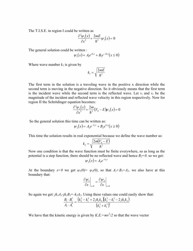
The T.I.S.E. in region I could be written as ( ) ( ) 02

1221

2

=+∂

∂ xmEx

x ψψh

The general solution could be written :

( ) ( )011111 ≤+= − xeBeAx xjkxjkψ

Where wave number k1 is given by

212h

mEk =

The first term in the solution is a traveling wave in the positive x direction while the second term is moving in the negative direction. So it obviously means that the first term is the incident wave while the second term is the reflected wave. Let v and vi r be the magnitude of the incident and reflected wave velocity in this region respectively. Now for region II the Schrödinger equation becomes:

( ) ( ) ( ) 022022

22

=−+∂

∂ xEVmx

x ψψh

So the general solution this time can be written as:

( ) ( )022222 ≥+= − xeBeAx xkxkψ

This time the solution results in real exponential because we define the wave number as:

( )2

02

2h

EVmk −=

Now one condition is that the wave function must be finite everywhere, so as long as the potential is a step function, there should be no reflected wave and hence B =0. so we get: B2

( ) xkeAx 222

−=ψ At the boundary x=0 we get ψ (0)= ψ (0), so that A +B =A1 2 1 1 2. we also have at this boundary that:

0

2

0

1

== ∂∂

=∂∂

xx xxψψ

So again we get: jk A -jk B1 1 1 B1=-k2A . Using these values one could easily show that: 2

( )( )( )22

122

212

12221

21

22

*11

*11 22

kkkjkkkkjkkk

AABB

+

−−+−=

⋅⋅

2/2 so that the wave vector We have that the kinetic energy is given by K.E.=mv

( )hhhh

mvvmmvmmEk ==== 2

222

21

22122

=vSo we can write the incident and reflected wave velocities as vi r=ħk1/m. Putting this

value in the expression of reflectance, we have: ( )

( ) 0.1422

122

22

21

221

22

*11

*11 =

+

+−=

⋅⋅⋅⋅

=kk

kkkkAAvBBvR

i

r

It seams that a lot of effort has been given for no apparent reason, as we could have arrived at the same conclusion classically that all the particles will eventually be reflected. But there are two rather astonishing observations, one that if it were that E<V0, even then we would have had some reflectance, and there remains a finite probability that the particles will penetrate the potential as A *.A2 2 has a finite value. This penetration into the barrier cannot be predicted classically. 2.7 Barrier potential and tunneling

quantum particles can tunnel trough the barrier and get out on the other side

E<U0 for left- side incident particle

k0 = p√(2mE)/ħ,

Tunneling

For wide barriers,

The tunneling rate is a very sensitive function of L

3 Energy bands in solids

3.1 Formation of bands in solid In atoms, electrons are distributed in orbitals, corresponding to certain energy. When two atoms come closely enough that their electrostatic field interact, then electrons from one atom feel the electric field of the other atom and their energy states change accordingly to accommodate for the forces from the second atom. In solids, atoms are so closely packed that huge numbers of atoms interact with each other. The result is that instead of a particular orbital, electrons now form bands of allowed energies corresponding to the orbitals, and we say to have energy bands in the solid.

Energy States & Energy Bands

222

4

2) 4 (

n

qmE

o

on

h

πε

− =

0/2/3

0100

11 arqa

−⎟⎟⎠

⎞⎜⎜⎝

⎛=

πψ

1

2

2

1

2

2

1

2

2

1s

2s

2

1

The potential wells due to the interactions between 2 atoms (in one molecule). Some electrons are shared between the atoms. Due to the interactions between electrons-electrons, nucleons-nucleons, and electrons-nucleons, the energy levels split, creating 1s, 2s, 2p,… doublets.

The potential experienced by an electron due to the coulomb interactions around an atom.

1s, 2s, 2p, are the energy levels that the electron can occupy.

Larger molecules, larger splitting.

In Solid with n≈ 1023 atoms, the sublevels are extremely close to each other. They coalesce and form an energy band. 1s, 2s, 2p… energy bands.

Non-Periodical Potential

r

r

)(rV

2)(rΨ

)(rVPeriodical Potential

r

r2)(rΨ

jkrerur ⋅=Ψ )()(

3.2 Electronic dispersion relation As we see from the previous topic that electrons see fast changing potentials due to the atomic cores of the solid. If the solid is bulk in nature, then the number of inner atoms surpass by far the number of surface atoms, and we can approximate the potential seen by the electron as perfectly periodic, and apply the Block’s theorem to determine the wave nature of the electron in a solid. →→→→

=Ψ rkjkk erUr .)()(

Where

)()(→→→

+= RrUrU kk Here we see that the periodicity of the potential arising from the crystal manifests itself in the magnitude of the electronic wavefunction.

)()()()( ...).(→→

+→→→→

Ψ==+=+Ψ→→→→→→→→→

reeerUeRrURr kRkjRkjrkj

kRrkj

kk What this means is that the electrons will be more probable to be around the center of the atomic nuclei. Now using the Krönig-Penny approximation, we could find the simplified wave function for the electron in 1D. The underlying mathematics is quite elementary and could be found in solid state texts, and only the result is presented herewith. We could see that how this model results in allowed energy bands and forbidden band gaps, between such two allowed bands. Such a sketch of the energy of a particle with respect to the wave vector, is know as the E-k Dispersion relation, or simply the dispersion relation. As one could easily translate wave vector k to momentum p using the wave particle duality principle, p=ħk this relation could be viewed as the relation

between energy and momentum of a particle, in this case of an electron in solid. If we reduce the dispersion relation to the first Brilloid zone. The mathematical definition of the brilloid zone involves the reciprocal lattice, but what it means is that when electrons are traveling within the solid, this is the first plane in a particular direction that the electrons are reflected. If we take a closer look at the dispersion relation of electrons, some point becomes eminent:

1. Within the range of the energy bands, electrons can have any energy, that is energy is continuous in the band.

2. For every energy that the electron can have, there is a momentum associated

with it, so electrons with different energy generally carries different momentum.

3. Conduction band being the highest unoccupied energy band, any electron

introduced into this band will tend to occupy the lowest possible energies. In the minima point, we see that the dispersion relation approximates the parabolic relation observed by the free electron, only with an effective mass associated with it. Indeed we can think of a conduction band electron to be free.

The apparent symmetry in the dispersion relation only exist for the 1D case, if we extend our system to 3D case, generally it results in different effective mass in different direction and also the crystal structure being different in different direction for general semiconductors, the dispersion relation is different in (100), (110) and (111) directions. It

is customary to express the extreme results in [111]and [100] direction to give dispersion relations as below:

3.3

The Concepts of: 1) Effective Mass

*2

2

2

11mdk

Ed=

h

2) Negative Mass 3) Positive charge 4) Holes

4. Density of states (DOS)

.1 Density of states

lectrical engineers eventually wish to describe the current-voltage characteristics of

.2 Bulk density of states

et us consider a particle trapped in a 3D potential well given by

for

4 Esemiconductor device. Since current is due to the flow of charge, an important step in the process is to determine the number of electrons and holes in the semiconductor that will be available for conduction. The number of carriers that can contribute to the conduction process is a function of the number of available energy or quantum states since, by Pauli’s exclusion principle, only one electron can occupy a given quantum state. We know that in forming bands in solid, the band of allowed energies are actually made up of discrete energy levels. So it becomes an important parameter how many states are there with a particular energy per unit volume of the solid. This density of electronic quantum energy states are called density of states (DOS). As we know in 3D there might be degenerate states with the same energy but different wave vector k, it then is only logical to calculate the density of state in k space and then convert it into energy space for a more accurate result. 4 L

( )( ) ∞=

=zyxVzyxV

,,0,,

elswhere

azayax <<<<<< 0,0,0

sing the separation of variable technique the Schrödinger’s equitation can be solved to U

give

( ) ⎟⎟⎠

⎞⎜⎜⎝

⎛++=++== 2

22222222

22

annnkkkkmE

zyxzyxπ

h

here nx, ny and nz are integers. As negative integers yield the same wavefunction with a W

negative value but the same probability, as long as quantum states are concerned, only positive integers are needed for a full description of possible k values. Now if we define a 3D k space, then only the one quadrant of positive kx, ky and kz components make up possible k states. As the quantum states are discrete, the distance between two states in k space in a particular dimension say x is:

( ) ( ) ⎟⎠⎞

⎜⎝⎛=⎟

⎠⎞

⎜⎝⎛−⎟

⎠⎞

⎜⎝⎛+=− nkk + aa

na xxxx

πππ11

Generalizing for 3 dimensions, the volume V a particular k state is Vk=(π/a)3. We can forknow determine the density of quantum states in k space. A differential volume in k space is given by 4πk2dk. So the differential density of quantum states in k space is given by:

( ) ( ) ( )3

221 42 adkkdkkdkkg π

== 238

aT ππ

ow converting the states into energy space we get, N

dEE

mdk2

1h

= hh

mEmE 222 kk 2 =⇒= and the differential

utting these values into the density of state equation in k space we get, P

( ) dEEmhammEa ⎞⎛ 2

3412 33 π( ) dEE

dEEgT ⋅=⋅⎟⎠

⎜⎝

= 22 322π hh

So the density of states in energy space becomes:

( ) ( ) Eh

m3

24πEg 3

2

=

.3 Density of states in thin films: 2D structures

very thin films, the quantum confinement is in one dimension, the direction of the

such that

4 Inthickness of the film and we are effectively dealing with a case of quantum well. Now in the confinement dimension, the energy becomes quantized to form discrete subbands far apart in energy from one another, so we can no longer assume band in that dimension. Suppose this dimension in the x direction, giving us effectively a 2Dimensional Electron Gas which is free to move in any direction in the y-z plane but are confined in the x dimension so that it has discrete k values and hence Ex x values. For the other dimensions contribution to the total energy we can deploy a similar strategy as before, only that this time we would be dealing in a in plane energy such that:

( ) ⎟⎟⎠

⎞⎜⎜⎝

⎛+=+== 2

2222222mE

zyppx EEEEEE +=→+= 2 annkkk zyzy

πh

Now we are effective dealing with a 2D system to give a 2D plane of k values with a differential area of Sk=(π/a)2 associated with each quantum state. Now we get

( ) ( ) ( )21 22 akdkkdkdkkg 24

aT ππ

π==

gain converting the k space into energy space we get, A

( ) dEhmadE

EmmEadEEgT 2

2

2

2 42

12 ππ

=⋅=hh

So the resultant density of states is given by

( ) 24h

mEg π=

4.4 Density of state in nanowire: 1D structure A nanowire is a one dimensional structure such that the two transverse dimensions confine the electrons in such a way that the only dimension the electron has a band nature left is the longitudinal direction. In the other two dimensions, its energy is quantized and has discrete subband values, giving rise to 2D subbands, while in the longitudinal direction, it has still the dispersion relation given by

( ) ⎟⎟⎠

⎞⎜⎜⎝

⎛=== 2

2222

22

ankkmE

zzπ

h

Now we get a 1D system which ultimately results in a length associated with every quantum state Lk=π/a and we get

( ) ( ) ( ) adk

a

dkdkkgT ππ == 212

Converting the k space to energy space we get,

( ) dEEm

hadE

EmadEEgT

22

1=⋅=

hπ

So finally we get the density of states as

( )Em

hEg 21

=

4.5 Density of states in Quantum Dots: 0D system In quantum dots, the confinement in 3 dimension:

pqrszyx EkkkE ,),,( = )()( , pqrsT EEEg −∝ δ is the cut-off energy of the subband pqr (p,q,r =1,2,3...) Where Es

5. Quantum viewpoint: Difference between bulk and nanostructure devices 5.1 Quantum confinement The basic difference in bulk and nanostructure devices is the spatial confinement of carriers. In bulk device, the energy states are so closely spaced that in the range of interest, they form a band, and the energy is said to be continuous in that band. The obvious implication is that since the carrier can now have continuous energy, in that range it can have a corresponding momentum in any direction. So they retain their Brownian motion to some extent. They are then treated as plane wave, free to move in any direction, and bound within the bulk material by electron affinity. The only interaction with the crystal to the apparently free carrier is incorporated in the effective mass part, which is usually different in different directions. The carriers loose their coherence by repeated scattering, and their phase information is completely destroyed, eliminating any significant quantum effect. The mean free path is larger than the Bohr radius of the carrier. If the semiconductor is non-degenerately doped, then the available states exceeds the available number of carriers significantly and the carriers interact like they were classical particles, and follow Maxwell-Boltzmann distribution. This usually associates ½ kBT energy for every degree of freedom, and thereby we can develop the device model treating carriers as classical particles. The basic current continuity equation can be approximated by the Boltzmann Transport Equation (BTE) and we get the general drift diffusion model for a bipolar device and field model for a unipolar device.

Since carriers are considered as free carriers with effective mass, and expressed as plane waves, it is apparent that they follow parabolic dispersion relation. This becomes clear as we look at the following dispersion relation in a band. The important part in current conduction and other electrical parameters for such devices concerns the electrons at the bottom of the conduction band and holes at the top of the conduction band. In both cases, to the extent of first approximation, the curvature of the dispersion relation can be approximated to be parabolic and our assumption of plane wave becomes valid. In nanostructure devices, this is not the case. Since the dimension(s) of the device becomes submicron, it effectively becomes lesser than the Bohr radius of the carrier in that particular direction(s). Even with phase altering scattering, the phase information is not completely randomized. So some coherence is retained, which means that some wave property of the carrier remains in effect, giving rise to significant quantum interaction among the carriers. Also, the system imposes short boundary to the dynamics of the carriers, bounding their motion in the direction(s) concerned. So the carriers becomes bounded, and no longer can be treated as plane wave. What this means is that now the carriers are no longer free particles which can roam around the device, but becomes localized and has preferred stationary positions of occupation. This effectively alters the carrier density and hence the current that it can carry. As the carriers becomes confined, the energy is also significantly quantized and the transitional energy increases in accordance. Thereby it can alter the optical properties of the nanostructure from its bulk counterpart. Depending upon the structure the confinement can be in a single direction, or in all three directions of propagation. 5.2 Quantum transport We need quantum mechanics to effectively arrive at the band theory for solids and ultimately this results in the physics of solid state devices and forms the basis of what we know about bulk devices. The same quantum mechanics is applied for nanostructure

devices for predicting the value of an observable in such devices. Though we apply QM for both scales, the difference in transport theory comes from the assumption that we make, which vary quite distinct in different scales. This results in semi-classical approach for the bulk device, while a full quantum mechanical approach is required in nanostructure devices. When we are dealing with solid state, we are in fact dealing with three distinct potentials. One is the macroscopic potential, which arises from applied bias and/or macroscopic localized space charges. The other two are microscopic potentials. One is the perfectly periodic potential of the crystal (for bulk devices), while the other is due to random scattering. For the effect of crystal, we incorporate the semi-classical quantity ‘effective mass’. The macroscopic potential deals with the band structure, and in the range of interest, it can be found using classical Newtonian laws of motion. Then the remaining scattering potential is the microscopic potential and treatment of this partially creates the difference between transport equations. In semi-classical theory, we assume that the scattering potential function of a single scatterer is calculated using Fermi’s Golden rule, and from the Schrödinger’s equation, while the macroscopic potential is found in terms of Newton’s laws. It neglects the interference between successive scatterers. This results in calculating the transmission probability from a Newtonistic viewpoint regarding current density, as well as using probability instead of probability amplitude in calculations. But as we go into nanoscale devices, we can no longer use the Fermi Golden rule for single point scatterer, but use only Schrödinger’s equation for this purpose. So effectively we can no longer ignore the position dependant interactive scatterers. The second difference is in these smaller devices, the macroscopic potential might be abrupt, so we have to consider quantum mechanical reflections, so Newtonian mechanics cannot be assumed. Then there is also the Hot Electron effect, due to which mobility and diffusivity becomes size dependant and functions of local field. All these contribute to the different transport mechanism for quantum transport from semiclassical transport. 5.3 Why Drift-diffusion equation fails for nanostructures For bulk device, we have to solve the current continuity equation

0=⋅∇ J And the Drift-diffusion equation

nqDqnJ ∇+= μξBut in nanosclale devices, this Drift-diffusion model fails due to two effects, the quantum effect and the hot electron effect.

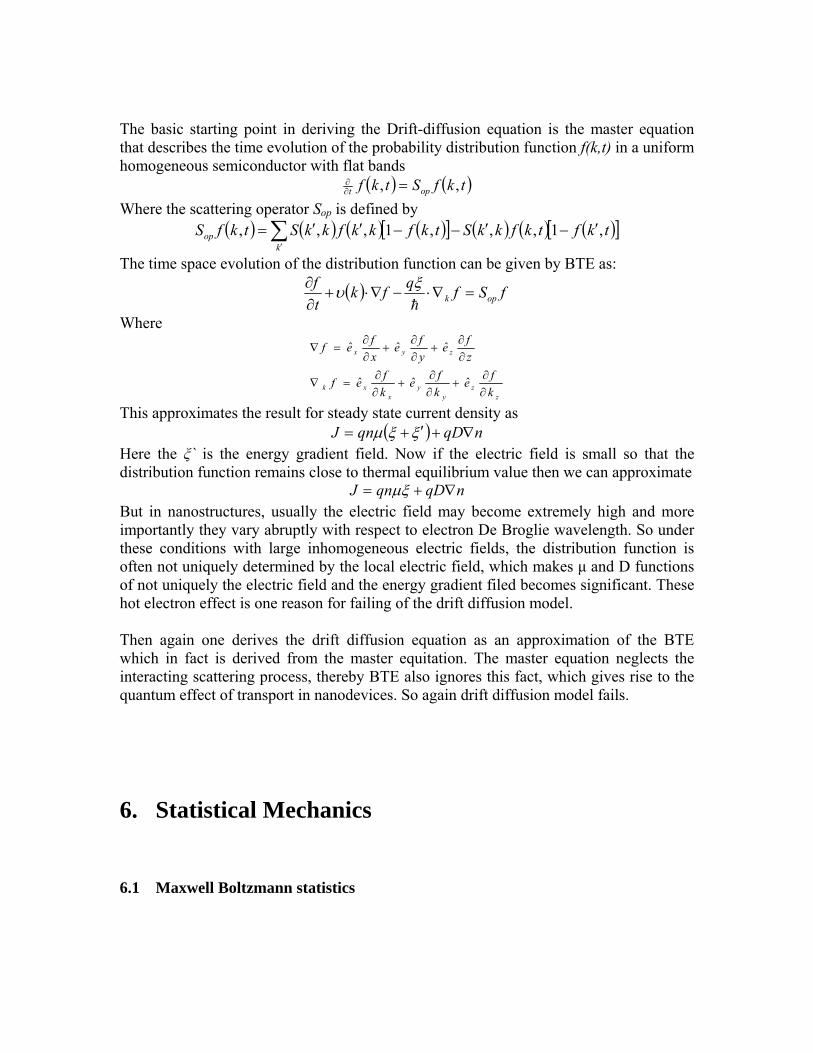
The basic starting point in deriving the Drift-diffusion equation is the master equation that describes the time evolution of the probability distribution function f(k,t) in a uniform homogeneous semiconductor with flat bands

( ) ( )tkfStkf opt ,, =∂∂

Where the scattering operator Sop is defined by ( ) ( ) ( ) ( )[ ] ( ) ( ) ( )[ ]∑

′

′−′−−′′=k

op tkftkfkkStkfkkfkkStkfS ,1,,,1,,,

The time space evolution of the distribution function can be given by BTE as:

( ) fSfqfktf

opk =∇⋅−∇⋅+∂∂

h

ξυ

Where

zz

yy

xxk

zyx

kfe

kfe

kfef

zfe

yfe

xfef

∂∂

+∂∂

+∂∂

=∇

∂∂

+∂∂

+∂∂

=∇

ˆˆˆ

ˆˆˆ

This approximates the result for steady state current density as ( ) nqDqnJ ∇+′+= ξξμ

Here the ξ` is the energy gradient field. Now if the electric field is small so that the distribution function remains close to thermal equilibrium value then we can approximate

nqDqnJ ∇+= μξBut in nanostructures, usually the electric field may become extremely high and more importantly they vary abruptly with respect to electron De Broglie wavelength. So under these conditions with large inhomogeneous electric fields, the distribution function is often not uniquely determined by the local electric field, which makes μ and D functions of not uniquely the electric field and the energy gradient filed becomes significant. These hot electron effect is one reason for failing of the drift diffusion model. Then again one derives the drift diffusion equation as an approximation of the BTE which in fact is derived from the master equitation. The master equation neglects the interacting scattering process, thereby BTE also ignores this fact, which gives rise to the quantum effect of transport in nanodevices. So again drift diffusion model fails. 6. Statistical Mechanics 6.1 Maxwell Boltzmann statistics

In statistical mechanics, Maxwell-Boltzmann statistics describes the statistical distribution of material particles over various energy states in thermal equilibrium, when the temperature is high enough and density is low enough to render quantum effects negligible. Maxwell-Boltzmann statistics are therefore applicable to almost any terrestrial phenomena for which the temperature is above a few tens of kelvins. The expected number of particles with energy ε for Maxwell-Boltzmann statistics is Ni i where:

where: Ni is the number of particles in state i εi is the energy of the i-th state gi is the degeneracy of state i, the number of microstates with energy εi μ is the chemical potential k is Boltzmann's constant T is absolute temperature N is the total number of particles

Z is the partition function

e(...) is the exponential function Equivalently, the distribution is sometimes expressed as

where the index i now specifies an individual microstate rather than the set of all states with energy εi Maxwell-Boltzmann statistics are often described as the statistics of "distinguishable" particles. In other words the configuration of particle A in state 1 and particle B in state 2 is different from the case where particle B is in state 1 and particle A is in state 2. When this idea is carried out fully, it yields the proper (Boltzmann) distribution of particles in the energy states. Suppose we have a number of energy levels, labelled by index i , each level having energy εi and containing a total of Ni particles. To begin with, lets ignore the degeneracy problem. Assume that there is only one way to put Ni particles into energy level i. The number of different ways of selecting one object from N objects is obviously N. The number of different ways of selecting 2 objects from N objects, in a particular order, is

thus N(N − 1) and that of selecting n objects in a particular order is seen to be N! / (N − n)!. The number of ways of selecting 2 objects from N objects without regard to order is N(N − 1) divided by the number of ways 2 objects can be ordered, which is 2!. It can be seen that the number of ways of selecting n objects from N objects without regard to order is the binomial coefficient: N! / n!(N − n)!. If we have a set of boxes numbered

, the number of ways of selecting N1 objects from N objects and placing them in box 1, then selecting N2 objects from the remaining N − N1 objects and placing them in box 2 etc. is

where the sum is over all boxes containing one or more objects. If the i-th box has a "degeneracy" of gi, that is, it has gi sub-boxes, such that any way of filling the i-th box where the number in the sub-boxes is changed is a distinct way of filling the box, then the number of ways of filling the i-th box must be increased by the number of ways of distributing the Ni objects in the gi boxes. The number of ways of placing Ni

distinguishable objects in gi boxes is . Thus the number of ways (W) that N atoms can be arranged in energy levels each level i having gi distinct states such that the i-th level has Ni atoms is:

For example, suppose we have three particles, a, b, and c, and we have three energy levels with degeneracies 1, 2, and 1 respectively. There are 6 ways to arrange the three particles

. . . . . . c . . c b . . b a . . aab ab ac ac bc Bc

The six ways are calculated from the formula:

We wish to find the set of Ni for which W is maximised, subject to the constraint that there be a fixed number of particles, and a fixed energy. The maxima of W and ln(W) occur at the value of Ni and, since it is easier to accomplish mathematically, we will maximise the latter function instead. We constrain our solution using Lagrange multipliers forming the function:

Using Stirling's approximation for the factorials and taking the derivative with respect to Ni, and setting the result to zero and solving for Ni yields the Maxwell-Boltzmann population numbers:

It can be shown thermodynamically that β = 1/kT where k is Boltzmann's constant and T is the temperature, and that α = -μ/kT where μ is the chemical potential, so that finally:

Note that the above formula is sometimes written:

where z = exp(μ / kT) is the absolute activity. Alternatively, we may use the fact that

to obtain the population numbers as

where Z is the partition function defined by:

6.2 Fermi Dirac distribution In statistical mechanics, Fermi-Dirac statistics determines the statistical distribution of fermions over the energy states for a system in thermal equilibrium. In other words, it is a probability of a given energy level to be occupied by a fermion. Fermions are particles which are indistinguishable and obey the Pauli exclusion principle, i.e., no more than one particle may occupy the same quantum state at the same time. Statistical thermodynamics is used to describe the behaviour of large numbers of particles. A collection of non-interacting fermions is called a Fermi gas. Fermi-Dirac (or F-D) statistics are closely related to Maxwell-Boltzmann statistics and Bose-Einstein statistics. While F-D statistics holds for fermions, B-E statistics plays the same role for bosons – the other type of particle found in nature. M-B statistics describes the velocity distribution of particles in a classical gas and represents the classical (high-temperature) limit of both F-D and B-E statistics. M-B statistics are particularly useful for studying gases, and B-E statistics are particularly useful when dealing with photons and other bosons. F-D statistics are most often used for the study of electrons in solids. As such, they form the basis of semiconductor device theory and electronics. The invention of quantum mechanics, when applied through F-D statistics, has made advances such as

the transistor possible. For this reason, F-D statistics are well-known not only to physicists, but also to electrical engineers. F-D statistics was introduced in 1926 by Enrico Fermi and Paul Dirac and applied in 1927 by Arnold Sommerfeld to electrons in metals. The expected number of particles in an energy state i for F-D statistics is

where: ni is the number of particles in state i εi is the energy of state i gi is the degeneracy of state i (the number of states with energy εi ) μ is the chemical potential. Sometimes the Fermi energy EF is used instead, as a low-temperature approximation. k is Boltzmann's constant T is absolute temperature Consider a two-level system, in which the excited state is an energy above the ground state. Because we are dealing with fermions, only one particle can occupy one energy level (quantum state). In other words, the energy contribution is either zero or . The partition function can be written

where i sums over all possible energy levels, gi is the degeneracy of the ith energy level, i.e. number of ways of getting/having that energy. As we have established before, there are only two possible energies: 0 and , both non-degenerate (gi = 1). So for this system the partition function is

. In general, probability of being in an energy state i is given by

So the probability of the energy level to be occupied by a particle, or the probability of a particle having energy is

One can also use the standardized formula for

For massive particles, all fermions are massive, zero energy is unachievable, we thus alter the formula to reflect that fact

where is the chemical potential of the system. At zero temperature, the chemical potential is exactly equal to the Fermi energy, EF. For systems well below the Fermi temperature, it is often sufficient to use ≈ EF. This formula is the Fermi-Dirac distribution.

6.3 Bose Einstein distribution

statistical mechanics, Bose-Einstein statisticsIn (or more colloquially B-E statistics) determines the statistical distribution of identical indistinguishable bosons over the energy states in thermal equilibrium. Bose-Einstein statistics are closely related to Maxwell-Boltzmann statistics (M-B) and Fermi-Dirac statistics (F-D). While F-D statistics holds for fermions, M-B statistics holds for classical particles, i.e. identical but distinguishable particles, and represents the classical or high-temperature limit of both F-D and B-E statistics. (M-B, B-E, and F-D statistics are all derived from the Boltzmann factor probability weight applied to the problem of classical particles and discrete energy quanta with boson/fermion behavior, respectively.) Bosons, unlike fermions, are not subject to the Pauli exclusion principle: an unlimited number of particles may occupy the same state at the same time. This explains why, at low temperatures, bosons can behave very differently than fermions; all the particles will tend to congregate together at the same lowest-energy state, forming what is known as a Bose-Einstein condensate. B-E statistics was introduced for photons in 1920 by Bose and generalized to atoms by Einstein in 1924. Einstein's original sketches were recovered in August 2005 in the Academical Library of Leiden, the Netherlands, where they were found by a student (Rowdy Boeyink). The expected number of particles in an energy state i for B-E statistics is:

with εi > μ and where: ni is the number of particles in state i gi is the degeneracy of state i εi is the energy of the i-th state μ is the chemical potential

k is Boltzmann's constant T is absolute temperature exp is the exponential function This reduces to M-B statistics for energies ( εi-μ ) >> kT. Suppose we have a number of energy levels, labelled by index i, each level having energy εi and containing a total of ni particles. Suppose each level contains gi distinct sublevels, all of which have the same energy, and which are distinguishable. For example, two particles may have different momenta, in which case they are distinguishable from each other, yet they can still have the same energy. The value of gi associated with level i is called the "degeneracy" of that energy level. Any number of bosons can occupy the same sublevel. Let w(n,g) be the number of ways of distributing n particles among the g sublevels of an energy level. There is only one way of distributing n particles with one sublevel, therefore w(n,1) = 1. Its easy to see that there are n + 1 ways of distributing n particles in two sublevels which we will write as:

With a little thought it can be seen that the number of ways of distributing n particles in three sublevels is w(n,3) = w(n,2) + w(n−1,2) + ... + w(0,2) so that

where we have used the following theorem involving binomial coefficients:

Continuing this process, we can see that w(n,g) is just a binomial coefficient

The number of ways that a set of occupation numbers ni can be realized is the product of the ways that each individual energy level can be populated:

where the approximation assumes that gi > > 1. Following the same procedure used in deriving the Maxwell-Boltzmann statistics, we wish to find the set of ni for which W is maximised, subject to the constraint that there be a fixed number of particles, and a fixed energy. The maxima of W and ln(W) occur at the value of Ni and, since it is easier to accomplish mathematically, we will maximise the latter function instead. We constrain our solution using Lagrange multipliers forming the function:

Using the gi > > 1 approximation and using Stirling's approximation for the factorials

and taking the derivative with respect to ni, and setting the result to zero and solving for ni yields the Fermi-Dirac population numbers:

It can be shown thermodynamically that β = 1/kT where k is Boltzmann's constant and T is the temperature, and that α = -μ/kT where μ is the chemical potential, so that finally:

Note that the above formula is sometimes written:

where z = exp(μ / kT) is the absolute activity. In the early 1920s Satyendra Nath Bose was intrigued by Einstein's theory of light waves being made of particles called photons. Bose was interested in deriving Planck's radiation formula, which Planck obtained largely by guessing. In 1900 Max Planck had derived his formula by manipulating the math to fit the empirical evidence. Using the particle picture of Einstein, Bose was able to derive the radiation formula by systematically developing a statistics of massless particles without the constraint of particle number conservation. Bose derived Planck's Law of Radiation by proposing different states for the photon. Instead of statistical independence of particles, Bose put particles into cells and described statistical independence of cells of phase space. Such systems allow two polarization states, and exhibit totally symmetric wavefunctions. He was quite successful in that he developed a statistical law governing the behaviour pattern of photons. However he was not able to publish his work, because no journals in Europe would accept his paper being unable to understand it. Bose sent his paper to Einstein who saw the significance of it and he used his influence to get it published. 7. Quantum Mechanics in nanostructures: some issues 7.1 Validity of effective mass approximation In bulk materials, most of the atoms reside well inside the surface, and we can in general consider surface to be a far away ending of otherwise periodic array of atoms. With this

view, the crystal can be thought to be effectively made of only periodic atoms, giving rise to periodic potential. With this approximation, one applies Bloch’s theorem and uses Krönig-Penny model to treat the macroscopic potential due to applied bias or macroscopic space charge, and gets the band diagrams of the material. A deeper investigation into the matter reveals that in the lowest parts of the conduction band, the energy dispersion relation is approximated to be parabolic. Now instead of explicitly determining the effect of the perfectly periodic crystal on conduction electron, one incorporates the idea of effective mass, which accounts for the crystal interaction at least near the band minima.

Effective mass is defined by analogy with Newton's second law . Using quantum mechanics it can be shown that for an electron in an external electric field E:

where a is acceleration, is reduced Planck's constant, , k is the wave

number (often loosely called momentum since k = ), ε(k) is the energy as a function of k, or the dispersion relation as it is often called. From the external electric field alone,

the electron would experience a force of , where q is the charge. Hence under the model that only the external electric field acts, effective mass m * becomes:

For a free particle, the dispersion relation is a quadratic, and so the effective mass would be constant (and equal to the real mass). In a crystal, the situation is far more complex. The dispersion relation is not even approximately quadratic, in the large scale. However, wherever a minimum occurs in the dispersion relation, the minimum can be approximated by a quadratic curve in the small region around that minimum. Hence, for electrons which have energy close to a minimum, effective mass is a useful concept. In energy regions far away from a minimum, effective mass can be negative or even approach infinity. Effective mass, being generally dependent on direction (with respect to the crystal axes), is a tensor. However, for most calculations the various directions can be averaged out. This concept of effective mass is valid for bulk materials where we can assume the crystal to be periodic, but in nanostructures the periodicity is no longer there as dimensions get smaller. Hence the band diagram also fails for nanostructure and we can no longer use the effective mass approximation. Experiments have shown that below 5 nm, we can no longer use the effective mass approximation. 7.2 Doping and effects in nanostructures In general doping is also a bulk concept where a very few (ppm or even ppb) of the the apparently huge number of semiconductor material atoms are replaced by dopants. This apparently small doping is enough to drastically change the conductive properties of the semiconductor. But in nanostructure, the number of semiconductor material could be small, specially in quantum dots, and a substitutional impurity should no longer be regarded as doping and a full quantum mechanical treatment is needed. But it has been experimentally found that still the concept of doping does remain somewhat valid in the range of QDs and p doped or n doped QD are readily available. Like dopants, defects also occur in bulk material in ppm or ppm ratio. So in quantum well or nanowire, defects has reduced probability of occurrence, while in quantum dots it practically is never there. 7.3 Surface Effects In bulk material, surface pose only as the loss of continuity in otherwise perfectly periodic crystal, hence surface is considered a defect. As the total number of atoms inside the volume is far larger than that at the surface, surface atoms only contribute to some

insignificant localized surface state. As the bonding is unsatisfied in the surface, so there remains dangling bond at the surface, which only plays some important part in the growth of the crystal. But in general surface has very little effect on a bulk semiconductor. But in nanostructures, the ratio of surface to volume is very high and a considerable number of atoms may constitute the surface for a nanowire or a quantum dot. In these cases, surface plays a very important part in its physical, chemical and electronic property. Some bulk indirect material becomes direct due to the surface recombination of electron holes, while some material conduct highly through the surface. In a semiconductor, the bands can be bent near the surface due to surface states. Under zero bias, the Fermi level has to be ‘level’, and this level typically goes through the surface states which lie in the band gap. Thus a p-type semiconductor has bands, which are bent downwards as you approach the surface. This leads to a reduction in the electron affinity. Some materials (eg Cs/p-type GaAs) can even be activated to negative electron affinity, and such materials form a potent source of electrons, which can also be spin-polarized as a result of the band structure. 7.4 Recombination Generally the recombination process in bulk semiconductor is band to band recombination, or Schottkey Hall Read recombination. But in nanostructures, we may find also Auger recombination and surface recombination. Direct band to band or intersubband recombination: Band-to-band recombination depends on the density of available electrons and holes. Both carrier types need to be available in the recombination process. Therefore, the rate is expected to be proportional to the product of n and p. Also, in thermal equilibrium, the recombination rate must equal the generation rate since there is no net recombination or generation. As the product of n and p equals n 2

i in thermal equilibrium, the net recombination rate can be expressed as:

Trap assisted recombination: Usually trap assisted recombination occurs in nanostructures of indirect material with confinement in one or two dimensions. The net recombination rate for trap-assisted recombination is given by:

Surface recombination: As surface states constitutes a large amount of the atoms or molecules in a nanostructure, this kind of recombination become significant in nanostructures. Recombination at surfaces and interfaces can have a significant impact on the behavior of such

semiconductor devices. This is because surfaces and interfaces typically contain a large number of recombination centers because of the abrupt termination of the semiconductor crystal, which leaves a large number of electrically active states. In addition, the surfaces and interfaces are more likely to contain impurities since they are exposed during the device fabrication process. The net recombination rate due to trap-assisted recombination and generation is given by:

This expression is almost identical to that of Shockley-Hall-Read recombination. The only difference is that the recombination is due to a two-dimensional density of traps, Nts, as the traps only exist at the surface or interface.

7.5 Hot Carrier Effects The term 'hot carriers' refers to either holes or electrons (also referred to as 'hot electrons') that have gained very high kinetic energy after being accelerated by a strong electric field in areas of high field intensities within a semiconductor (especially MOS) device. Because of their high kinetic energy, hot carriers can get injected and trapped in areas of the device where they shouldn't be, forming a space charge that causes the device to degrade or become unstable. The term 'hot carrier effects', therefore, refers to device degradation or instability caused by hot carrier injection. According to the 5th Edition Hitachi Semiconductor Device Reliability Handbook, there are four (4) commonly encountered hot carrier injection mechanisms. These are 1) the drain avalanche hot carrier injection; 2) the channel hot electron injection; 3) the substrate hot electron injection; and 4) the secondary generated hot electron injection. The drain avalanche hot carrier (DAHC) injection is said to produce the worst device degradation under normal operating temperature range. This occurs when a high voltage applied at the drain under non-saturated conditions (VD>VG) results in very high electric fields near the drain, which accelerate channel carriers into the drain's depletion region. Studies have shown that the worst effects occur when VD = 2VG. The acceleration of the channel carriers causes them to collide with Si lattice atoms, creating dislodged electron-hole pairs in the process. This phenomenon is known as impact ionization, with some of the displaced e-h pairs also gaining enough energy to overcome the electric potential barrier between the silicon substrate and the gate oxide. Under the influence of drain-to-gate field, hot carriers that surmount the substrate-gate oxide barrier get injected into the gate oxide layer where they are sometimes trapped.

This hot carrier injection process occurs mainly in a narrow injection zone at the drain end of the device where the lateral field is at its maximum. 7.6 Coulomb Blockade In physics, a Coulomb blockade, named after Charles-Augustin de Coulomb, is the increased resistance at small bias voltages of an electronic device comprising at least one low-capacitance tunnel junction. A tunnel junction is, in its simplest form, a thin insulating barrier between two conducting electrodes. If the electrodes are superconducting, Cooper pairs with a charge of two elementary charges carry the current. In the case that the electrodes are normalconducting, i.e. neither superconducting nor semiconducting, electrons with a charge of one elementary charge carry the current. The following reasoning is for the case of tunnel junctions with an insulating barrier between two normalconducting electrodes (NIN junctions).

Schematic representation of an electron tunnelling through a barrier According to the laws of classical electrodynamics, no current can flow through an insulating barrier. According to the laws of quantum mechanics, however, there is a finite (larger than zero) probability for an electron on one side of the barrier to reach the other side. When a bias voltage is applied, this means that there will be a current flow. In first-order approximation, that is, neglecting additional effects, the tunnelling current will be proportional to the bias voltage. In electrical terms, the tunnel junction behaves as a resistor with a constant resistance, also known as an ohmic resistor. The resistance depends exponentially on the barrier thickness. Typical barrier thicknesses are on the order of one to several nanometers. An arrangement of two conductors with an insulating layer in between not only has a resistance, but also a finite capacitance. The insulator is also called dielectric in this context, the tunnel junction behaves as a capacitor. Due to the discreteness of electrical charge, current flow through a tunnel junction is a series of events in which exactly one electron passes (tunnels) through the tunnel barrier (we neglect events in which two electrons tunnel simultaneously). The tunnel junction capacitor is charged with one elementary charge by the tunnelling electron, causing a voltage buildup U = e / C, where e is the elementary charge of 1.6×10-19 coulomb and C

the capacitance of the junction. If the capacitance is very small, the voltage buildup can be large enough to prevent another electron from tunnelling. The electrical current is then suppressed at low bias voltages and the resistance of the device is no longer constant. The increase of the differential resistance around zero bias is called the Coulomb blockade. In order for the Coulomb blockade to be observable, the temperature has to be low enough so that the characteristic charging energy (the energy that is required to charge the junction with one elementary charge) is larger than the thermal energy of the charge carriers. For capacitances below 1 femtofarad (10-15 farad), this implies that the temperature has to be below about 1 kelvin. This temperature range is routinely reached for example by dilution refrigerators.

Energylevels of source, island and drain (from left to right) in a single electron transistor

for both the blocking state (upper part) and the transmitting state (lower part).

Single electron transistor with niobium leads and aluminium island To make a tunnel junction in plate condenser geometry with a capacitance 1 femtofarad, using an oxide layer of electric permeability 10 and thickness one nanometer, one has to create electrodes with dimensions of approximately 100 by 100 nanometers. This range of dimensions is routinely reached for example by electron beam lithography and appropriate pattern transfer technologies, like the Niemeyer-Dolan technique, also known as shadow evaporation technology.

Another problem for the observation of the Coulomb blockade is the relatively large capacitance of the leads that connect the tunnel junction to the measurement electronics. The simplest device in which the effect of Coulomb blockade can be observed is the so-called single electron transistor. It consists of two tunnel junctions sharing one common electrode with a low self-capacitance, known as the island. The electrical potential of the island can be tuned by a third electrode (the gate), capacitively coupled to the island. In the blocking state no accessible energy levels are within tunneling range of the electron (red) on the source contact. All energy levels on the island electrode with lower energies are occupied. When a positive voltage is applied to the gate electrode the energy levels of the island electrode are lowered. The electron (green 1.) can tunnel onto the island (2.), occupying a previously vaccant energy level. From there it can tunnel onto the drain electrode (3.) where it inelastically scatters and reaches the drain electrode Fermi level (4.). The energy levels of the island electrode are evenly spaced with a separation of ΔE. ΔE is the energy needed to each subsequent electron to the island, which acts as a self-capacitance C. The lower C the bigger ΔE gets. It is crucial for ΔE to be larger than the energy of thermal fluctuations KBT, otherwise an electron from the source electrode can always be thermally excited onto an unoccupied level of the island electrode, and no blocking can be observed.