1 balanced search trees (walls & mirrors - chapter 12 & end of chapter 10)
Post on 22-Dec-2015
220 views
TRANSCRIPT
1
Balanced Search Trees
(Walls & Mirrors - Chapter 12 &
end of Chapter 10)
2
If you don’t find it in the Index, look very carefully through the entire catalogue.
– Consumer’s Guide, Sears, Roebuck & Co. (1897)
One mustn’t ask apple trees for oranges.
– Gustave Flaubert (Pensées de Gustave Flaubert)
A fool sees not the same tree that a wise man sees.
– William Blake (The Marriage of Heaven and Hell)

3
A tree’s a tree. How many more do you need to look at?
– Ronald Reagan (Speech, Sept. 12, 1965)
4
Overview
• Building a Minimum-Height Binary Search Tree
• 2-3 Trees
• 2-3-4 Trees
• Red-Black Trees
• AVL Trees
• General Trees
• N-ary Trees

5
Balanced Binary Trees
• Recall that a binary tree is balanced if the difference in height between any node’s left and right subtree is 1.

6
Balanced Search Trees• If a binary search tree containing n nodes is balanced,
insertion, deletion and retrieval will all take O( log n ) time.
• Otherwise, each of these operations could take O( n ) time, which is no better than a sequential search through a linked list.
40
20 60
10 30 50
balanced
20
30
10
40
50
60unbalanced

7
Building a Minimum-HeightBinary Search Tree
Basic idea:
1) Write items, in sorted order, from a binary search tree to a file using inorder traversal.
2) Invoke buildtree, which
a) Creates a new tree node, t ;
b) Calls itself recursively to read half of the items from the file and place them in t ’s left subtree; and then
c) Calls itself recursively to read the remaining items and place them in t ’s right subtree.
When step 2 completes, t will be the root of a (balanced) minimum-height binary search tree.

8
Building a Min-Height Binary Search Tree: Algorithm
// build a minimum-height binary search tree from n items in a file// sorted by search-key; treePtr will point to the tree’s root
buildTree( TreeNode *&treePtr, int n )
{ if( n > 0 )
{ treePtr = new TreeNode; // create a new TreeNode
treePtr -> leftChild = treePtr -> rightChild = NULL;
buildTree( treePtr -> leftChild, n/2 ); // build left subtree
readItem( treePtr -> item ); // get next item from input file
buildTree( treePtr -> rightChild, (n – 1)/2 ); // build right subtree }}

9
Building a Min-Height Binary Search Tree
Unbalancedbinary search tree
20
10 30
25
22
35
40
50
60
• Items from the tree are written to a file using inorder traversal, placing them in the following order:
10, 20, 22, 25, 30, 35, 40, 50, 60
• buildTree is invoked with n = 9, which:
– creates a new node, t1 ;
– calls itself recursively with t1’s leftChild pointer and n = [ 9/2 ] = 4.
[ x ] denotes the greatest integer in x
10
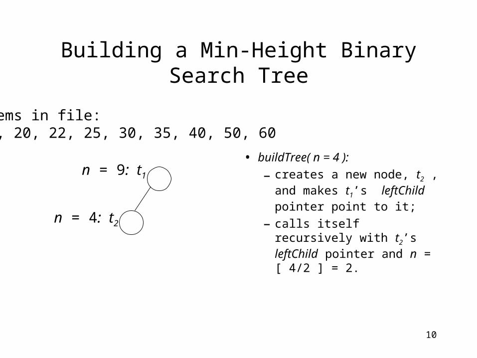
Building a Min-Height Binary Search Tree
• buildTree( n = 4 ):
– creates a new node, t2 , and makes t1’s leftChild pointer point to it;
– calls itself recursively with t2’s leftChild pointer and n = [ 4/2 ] = 2.
Items in file:10, 20, 22, 25, 30, 35, 40, 50, 60
n = 9: t1
n = 4: t2

11
Building a Min-Height Binary Search Tree
• buildTree( n = 2 ):
– creates a new node, t3 , and makes t2’s leftChild pointer point to it;
– calls itself recursively with t3’s leftChild pointer and n = [ 2/2 ] = 1.
Items in file:10, 20, 22, 25, 30, 35, 40, 50, 60
n = 9: t1
n = 4: t2
n = 2: t3
12
Building a Min-Height Binary Search Tree
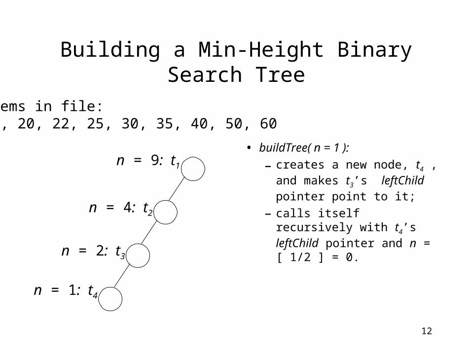
• buildTree( n = 1 ):
– creates a new node, t4 , and makes t3’s leftChild pointer point to it;
– calls itself recursively with t4’s leftChild pointer and n = [ 1/2 ] = 0.
Items in file:10, 20, 22, 25, 30, 35, 40, 50, 60
n = 9: t1
n = 4: t2
n = 2: t3
n = 1: t4

13
Building a Min-Height Binary Search Tree
• buildtree( n = 0 ):
– returns immediately to the place where it was called.
• buildTree( n = 1 ):
– reads the first item (= 10) from the input file and stores it in t4 ;
– calls itself recursively with t4’s rightChild pointer and n = [ (1 – 1) / 2 ] = 0.
Items in file:10, 20, 22, 25, 30, 35, 40, 50, 60
n = 9: t1
n = 4: t2
n = 2: t3
10n = 1: t4
14
Building a Min-Height Binary Search Tree
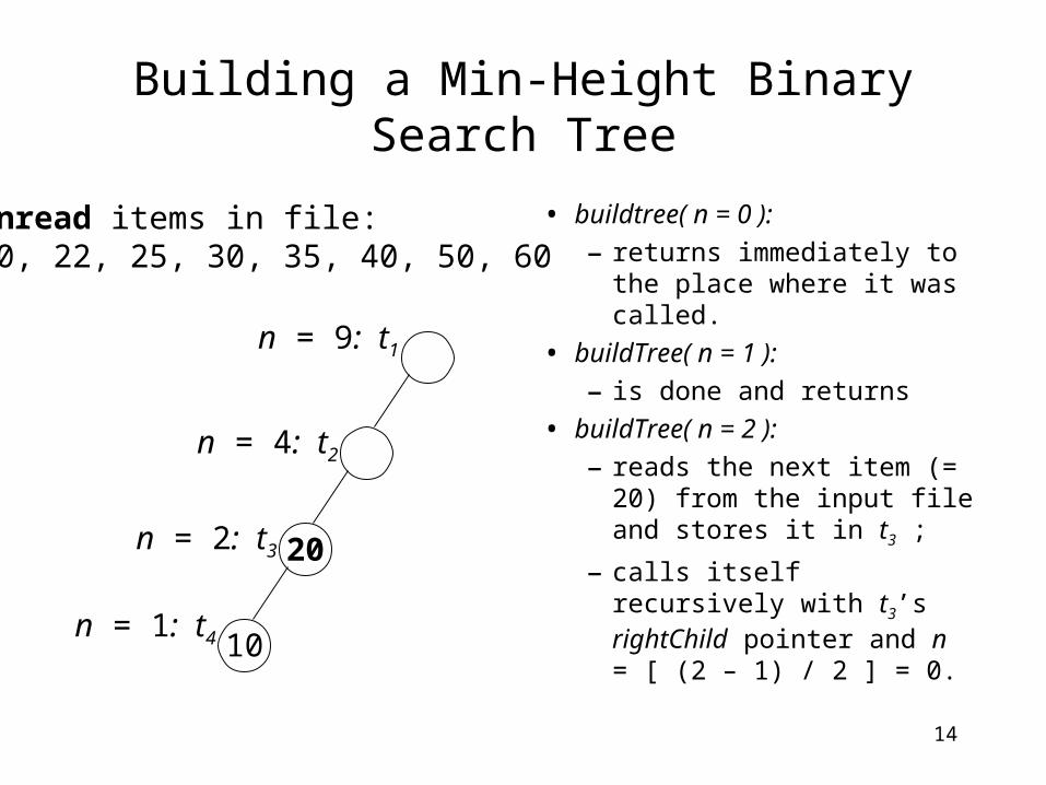
• buildtree( n = 0 ):
– returns immediately to the place where it was called.
• buildTree( n = 1 ):
– is done and returns
• buildTree( n = 2 ):
– reads the next item (= 20) from the input file and stores it in t3 ;
– calls itself recursively with t3’s rightChild pointer and n = [ (2 – 1) / 2 ] = 0.
Unread items in file:20, 22, 25, 30, 35, 40, 50, 60
n = 9: t1
n = 4: t2
20n = 2: t3
10n = 1: t4

15
Building a Min-Height Binary Search Tree
Unread items in file:22, 25, 30, 35, 40, 50, 60
22
n = 9: t1
n = 4: t2
20n = 2: t3
10n = 1: t4
• buildtree( n = 0 ):
– returns immediately
• buildTree( n = 2 ):
– is done and returns
• buildTree( n = 4 ):
– reads the next item (= 22) from the input file and stores it in t2 ;
– calls itself recursively with t2’s rightChild pointer and n = [ (4 – 1)/2 ] = 1.
16
Building a Min-Height Binary Search Tree
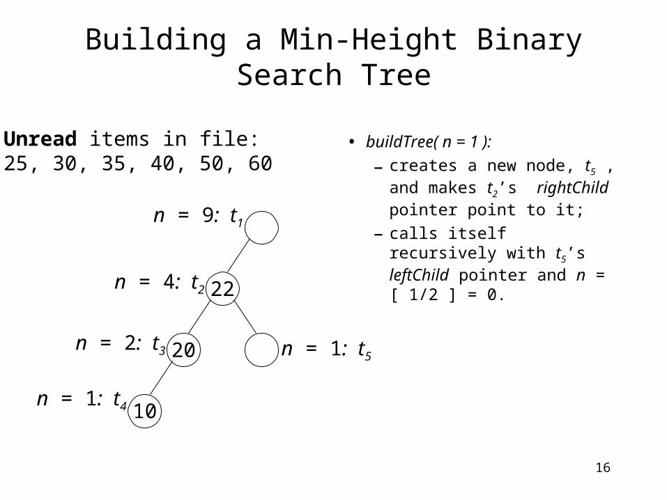
Unread items in file:25, 30, 35, 40, 50, 60
• buildTree( n = 1 ):
– creates a new node, t5 , and makes t2’s rightChild pointer point to it;
– calls itself recursively with t5’s leftChild pointer and n = [ 1/2 ] = 0.
20
22
n = 9: t1
n = 4: t2
n = 2: t3
10n = 1: t4
n = 1: t5

17
Building a Min-Height Binary Search Tree
Unread items in file:25, 30, 35, 40, 50, 60
• buildtree( n = 0 ):
– returns immediately
• buildTree( n = 1 ):
– reads the next item (= 25) from the input file and stores it in t5 ;
– calls itself recursively with t5’s rightChild pointer and n = [ (1 – 1) / 2 ] = 0.
20
22
n = 9: t1
n = 4: t2
n = 2: t3
10n = 1: t4
25
n = 1: t5
18
Building a Min-Height Binary Search Tree
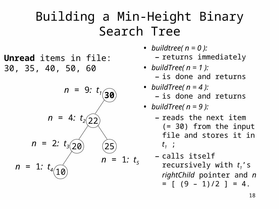
Unread items in file:30, 35, 40, 50, 60
• buildtree( n = 0 ):– returns immediately
• buildTree( n = 1 ):– is done and returns
• buildTree( n = 4 ):– is done and returns
• buildTree( n = 9 ):
– reads the next item (= 30) from the input file and stores it in t1 ;
– calls itself recursively with t1’s rightChild pointer and n = [ (9 – 1)/2 ] = 4.
20
30
22
n = 9: t1
n = 4: t2
n = 2: t3
10n = 1: t4
25
n = 1: t5
19
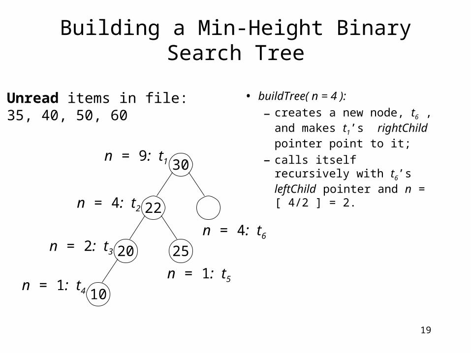
Building a Min-Height Binary Search Tree
Unread items in file:35, 40, 50, 60
• buildTree( n = 4 ):
– creates a new node, t6 , and makes t1’s rightChild pointer point to it;
– calls itself recursively with t6’s leftChild pointer and n = [ 4/2 ] = 2.
20
30
22
n = 9: t1
n = 4: t2
n = 2: t3
10n = 1: t4
25
n = 1: t5
n = 4: t6

20
Building a Min-Height Binary Search Tree
Unread items in file:35, 40, 50, 60
• buildTree( n = 2 ):
– creates a new node, t7 , and makes t6’s leftChild pointer point to it;
– calls itself recursively with t7’s leftChild pointer and n = [ 2/2 ] = 1.
20
30
22
n = 9: t1
10
25 n = 2: t7
n = 4: t6

21
Building a Min-Height Binary Search Tree
Unread items in file:35, 40, 50, 60
• buildTree( n = 1 ):
– creates a new node, t8 , and makes t7’s leftChild pointer point to it;
– calls itself recursively with t8’s leftChild pointer and n = [ 1/2 ] = 0.
20
30
22
n = 9: t1
10
25 n = 2: t7
n = 4: t6
n = 1: t8

22
Building a Min-Height Binary Search Tree
Unread items in file:35, 40, 50, 60
• buildtree( n = 0 ):
– returns immediately.
• buildTree( n = 1 ):
– reads the next item (= 35) from the input file and stores it in t8 ;
– calls itself recursively with t8’s rightChild pointer and n = [ (1 – 1) / 2 ] = 0.
20
30
22
n = 9: t1
10
25 n = 2: t7
n = 4: t6
35 n = 1: t8

23
Building a Min-Height Binary Search Tree
Unread items in file:40, 50, 60
20
30
22
n = 9: t1
10
25 n = 2: t7
n = 4: t6
40
35 n = 1: t8
• buildtree( n = 0 ):– returns immediately
• buildTree( n = 1 ):– is done and returns
• buildTree( n = 2 ):
– reads the next item (= 40) from the input file and stores it in t7 ;
– calls itself recursively with t7’s rightChild pointer and n = [ (2 – 1)/2 ] = 0.

24
Building a Min-Height Binary Search Tree
Unread items in file:50, 60
50
20
30
22
n = 9: t1
10
25 n = 2: t7
n = 4: t6
40
35 n = 1: t8
• buildtree( n = 0 ):– returns immediately
• buildTree( n = 2 ):– is done and returns
• buildTree( n = 4 ):
– reads the next item (= 50) from the input file and stores it in t6 ;
– calls itself recursively with t6’s rightChild pointer and n = [ (4 – 1)/2 ] = 1.

25
Building a Min-Height Binary Search Tree
Unread items in file:60
• buildTree( n = 1 ):
– creates a new node, t9 , and makes t6’s rightChild pointer point to it;
– calls itself recursively with t9’s leftChild pointer and n = [ 1/2 ] = 0.50
20
30
22
n = 9: t1
10
25
n = 4: t6
40
35
n = 1: t9

26
Building a Min-Height Binary Search Tree
Unread items in file:60
50
20
30
22
n = 9: t1
10
25
n = 4: t6
40
35
60
n = 1: t9
• buildtree( n = 0 ):– returns immediately
• buildTree( n = 1 ):
– reads the next item (= 60) from the input file and stores it in t9 ;
– calls itself recursively with t9’s rightChild pointer and n = [ (1 – 1)/2 ] = 0.

27
Building a Min-Height Binary Search Tree
No Unread items in file
50
20
30
22
n = 9: t1
10
25
n = 4: t6
40
35
60
n = 1: t9
• buildtree( n = 0 ):
– returns immediately
• buildTree( n = 1 ):
– is done and returns
• buildTree( n = 4 ):
– is done and returns
• buildTree( n = 9 ):
– is done and returns, having created a minimum height binary search tree from items read from the input file.

28
Building a Min-Height Binary Search Tree• buildtree is guaranteed to produce a minimum-height binary
search tree. That is,
– a tree with n nodes will have height log2 (n + 1) .
• Although the tree will be balanced, it will not necessarily be complete.
• However, searching, inserting and deleting items from a binary search tree can be efficient as long as the tree remains balanced – it is not necessary for the tree to be complete.
• One strategy for maintaining a balanced binary search tree is to periodically (e.g. overnight or over a weekend) dump the tree to a file and rebuild the tree.
• Another strategy is to maintain the tree’s balance while insertions and deletions are being done. We shall spend the remainder of the lecture considering this strategy.

29
2-3 Tree
• Intuitively, a 2-3 tree is a tree in which each parent node has either 2 or 3 children, and all leaves are at the same level.
• According to Donald Knuth, 2-3 trees were invented by John E. Hopcroft.
30
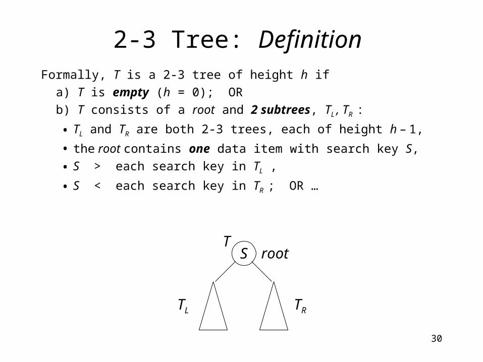
2-3 Tree: DefinitionFormally, T is a 2-3 tree of height h if
a) T is empty (h = 0); OR
b) T consists of a root and 2 subtrees, TL , TR :
• TL and TR are both 2-3 trees, each of height h – 1,
• the root contains one data item with search key S,
• S > each search key in TL ,
• S < each search key in TR ; OR …
S
TL TR
rootT

31
2-3 Tree: Definition (Cont’d.)
c) T consists of a root and 3 subtrees, TL , TM , TR :
• TL , TM , TR are all 2-3 trees, each of height h – 1,
• the root contains two data items with search keys S and L,
• each search key in TL < S < each search key in TM ,
• each search key in TM < L < each search key in TR .
TL TR
rootT
TM
S L
32
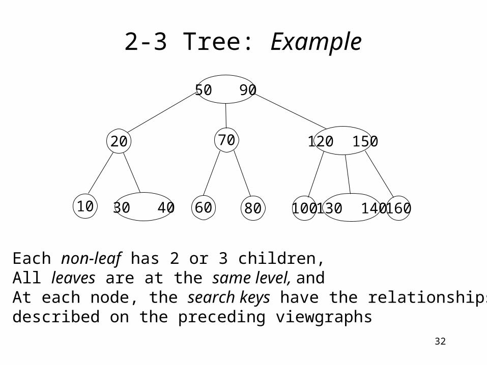
2-3 Tree: Example
50 90
20 70 120 150
10 60 80 100 130 140 16030 40
• Each non-leaf has 2 or 3 children,• All leaves are at the same level, and• At each node, the search keys have the relationships described on the preceding viewgraphs

33
2-3 Tree: Efficiency
• Insertion and deletion can be defined so that the 2-3 tree remains balanced and its other properties are maintained.
• In particular, a 2-3 tree with n nodes never has a height greater than log2 (n + 1) , which is the same as the minimum height of a binary tree with n nodes.
• Consequently, finding an item in a 2-3 tree is never worse than O( log n), regardless of the insertions or deletions that were done previously.
34
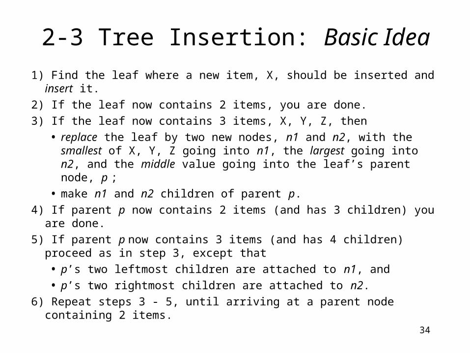
2-3 Tree Insertion: Basic Idea
1) Find the leaf where a new item, X, should be inserted and insert it.
2) If the leaf now contains 2 items, you are done.
3) If the leaf now contains 3 items, X, Y, Z, then
• replace the leaf by two new nodes, n1 and n2, with the smallest of X, Y, Z going into n1, the largest going into n2, and the middle value going into the leaf’s parent node, p ;
• make n1 and n2 children of parent p.
4) If parent p now contains 2 items (and has 3 children) you are done.
5) If parent p now contains 3 items (and has 4 children) proceed as in step 3, except that
• p’s two leftmost children are attached to n1, and
• p’s two rightmost children are attached to n2.
6) Repeat steps 3 - 5, until arriving at a parent node containing 2 items.

35
2-3 Tree Insertion: Example
30 39
10 20 37 38 40
30 39
10 20 36 37 38 40
• Insert 36

36
2-3 Tree Insertion: Example (Cont’d.)
• Since the leaf with 36 in it now contains 3 items, replace the leaf by two new nodes containing 36 (the smallest) and 38 (the largest).
• Move 37 (the middle value) up to its parent, p.
• Make nodes containing 36 and 38 children of parent, p.
30 37 39
10 20 4036 38
p
30 39
10 20 36 37 38 40
p
37
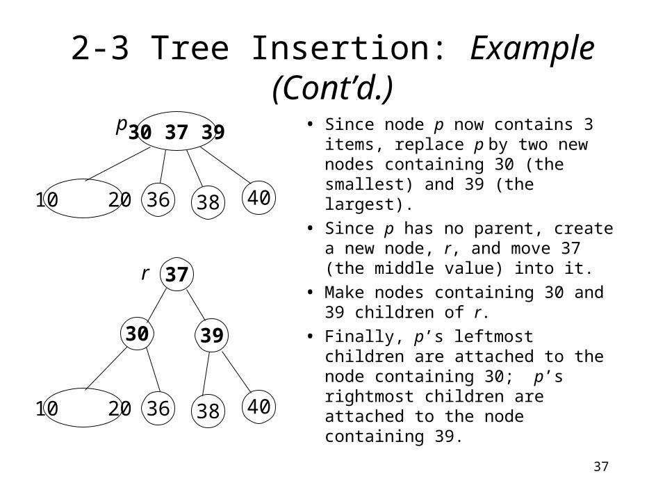
2-3 Tree Insertion: Example (Cont’d.)
• Since node p now contains 3 items, replace p by two new nodes containing 30 (the smallest) and 39 (the largest).
• Since p has no parent, create a new node, r, and move 37 (the middle value) into it.
• Make nodes containing 30 and 39 children of r.
• Finally, p’s leftmost children are attached to the node containing 30; p’s rightmost children are attached to the node containing 39.
30 37 39
10 20 4036 38
p
10 20 4036 38
30 39
37r

38
2-3 Tree Insertion: Algorithm
// insert newItem into 2-3 Tree, ttTree
insertItem( Two3Tree ttTree, ItemType newItem ){
KeyType searchKey = getKey( newItem );
/* find the leaf, leafNode, in which searchKey belongs */
/* add newItem to leafNode */
if( /* leafNode now contains 3 items */ )
splitNode( leafNode );
}

39
2-3 Tree Insertion: Algorithm (Cont’d.)splitNode( TreeNode n ){ if( /* n is the root of a tree */ ) /* create a new TreeNode, p */ else /* set p to the parent of n */
/* replace node n by n1 and n2, with p as their parent; */ /* give n1 the item in n with the smallest search key; */ /* give n2 the item in n with the largest search key */
if( /* n is not a leaf */ ) { /* make n1 the parent of n’s two leftmost children */ /* make n2 the parent of n’s two rightmost children */ }
/* give node p the item in n with the middle search key */
if( /* p now contains 3 items */ ) splitNode( p );}

40
2-3 Tree: Remarks
• If a 2-3 tree needs to grow after inserting an item, it grows upwards at the root.
• Deletion from a 2-3 tree is a bit more complicated than insertion, involving merging nodes and redistributing items. Refer to Chapter 12 of Walls & Mirrors for details.

41
2-3-4 Tree
• A 2-3-4 tree is an extension to the concept of a 2-3 tree:
– each parent node has up to 4 children,
– all leaves are at the same level,
– each node can contain up to 3 items.
• Insertions and deletions in a 2-3-4 tree require fewer steps than in a 2-3 tree.
42
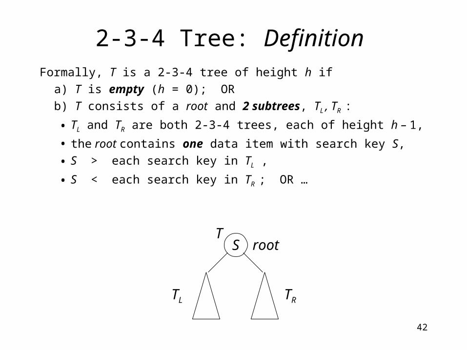
2-3-4 Tree: DefinitionFormally, T is a 2-3-4 tree of height h if
a) T is empty (h = 0); OR
b) T consists of a root and 2 subtrees, TL , TR :
• TL and TR are both 2-3-4 trees, each of height h – 1,
• the root contains one data item with search key S,
• S > each search key in TL ,
• S < each search key in TR ; OR …
S
TL TR
rootT

43
2-3-4 Tree: Definition (Cont’d.)
c) T consists of a root and 3 subtrees, TL , TM , TR :
• TL , TM , TR are all 2-3-4 trees, each of height h – 1,
• the root contains two data items with search keys S and L,
• each search key in TL < S < each search key in TM ,
• each search key in TM < L < each search key in TR ; OR …
TL TR
rootT
TM
S L

44
2-3-4 Tree: Definition (Cont’d.)d) T consists of a root and 4 subtrees, TL , TML , TMR , TR :
• TL , TML , TMR , TR are all 2-3-4 trees, each of height h – 1,
• the root contains three data items with search keys S, M and L,
• each search key in TL < S < each search key in TML ,
• each search key in TML < M < each search key in TMR ,
• each search key in TMR < L < each search key in TR .
TL TR
S M LT
root
TML TMR

45
2-3-4 Tree: Example
30 70
255 15 75 11085 95
10 20
40 60
50 80 90 100
• each parent node has up to 4 children
• each node contains up to 3 items
• all leaves are at the same level
• the search keys have the relationships described on the preceding viewgraphs
46
2-3-4 Tree Insertion: Strategy
• When one inserts a new item into a 2-3 tree, the intended destination node is split when it overflows. Steps are then taken, recursively, to determine whether any ancestor of this node also needs to be split.
• While searching for the place to insert a new item into a 2-3-4 tree, any node encountered containing 3 items (and 4 children) is immediately split before the destination node is found.
• This difference ensures that when the destination node in a 2-3-4 tree is finally found, there will be room in the node for the new item, and ancestor nodes do not need to be revisited.
• This difference also simplifies the insertion algorithm for a 2-3-4 tree.
47
2-3-4 Tree Insertion: Basic Idea
1) Search for the leaf where a new item, W, should be inserted.
2) If a node, n, containing 3 items, X, Y, Z, is encountered, then
• replace n by two new nodes, n1 and n2, with the smallest of X, Y, Z going into n1, the largest going into n2, and the middle value going into n’s parent node, p ;
• if p does not exist (n is also a root), create a new node p ;
• make n1 and n2 children of parent p.
3) If W’s search key < search key of middle( X, Y, Z ), then continue searching with node n1. Otherwise, continue searching with node n2.
4) When the destination leaf is found, it will contain 1 or 2 items. Insert W, and you are done.
48
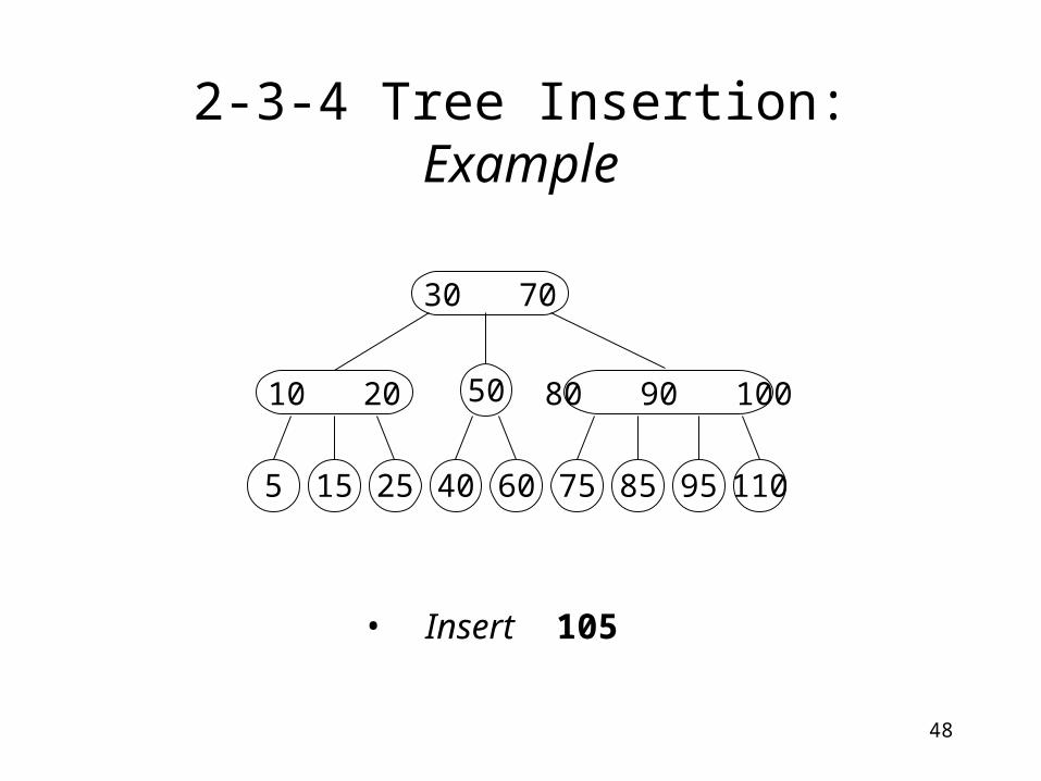
2-3-4 Tree Insertion: Example
30 70
255 15 75 11085 95
10 20
40 60
50 80 90 100
• Insert 105

49
2-3-4 Tree Insertion: Example
• While searching for the leaf into which 105 can be inserted, node n containing 3 items is encountered.
• Replace n by two new nodes, n1, containing 80 (the smallest) and n2, containing 100 (the largest).
• Move 90 (the middle value) up to its parent, p.
• Make n1 and n2 children of p.
30 70
255 15 75 11085 95
10 20
40 60
50 80 90 100 n
p

50
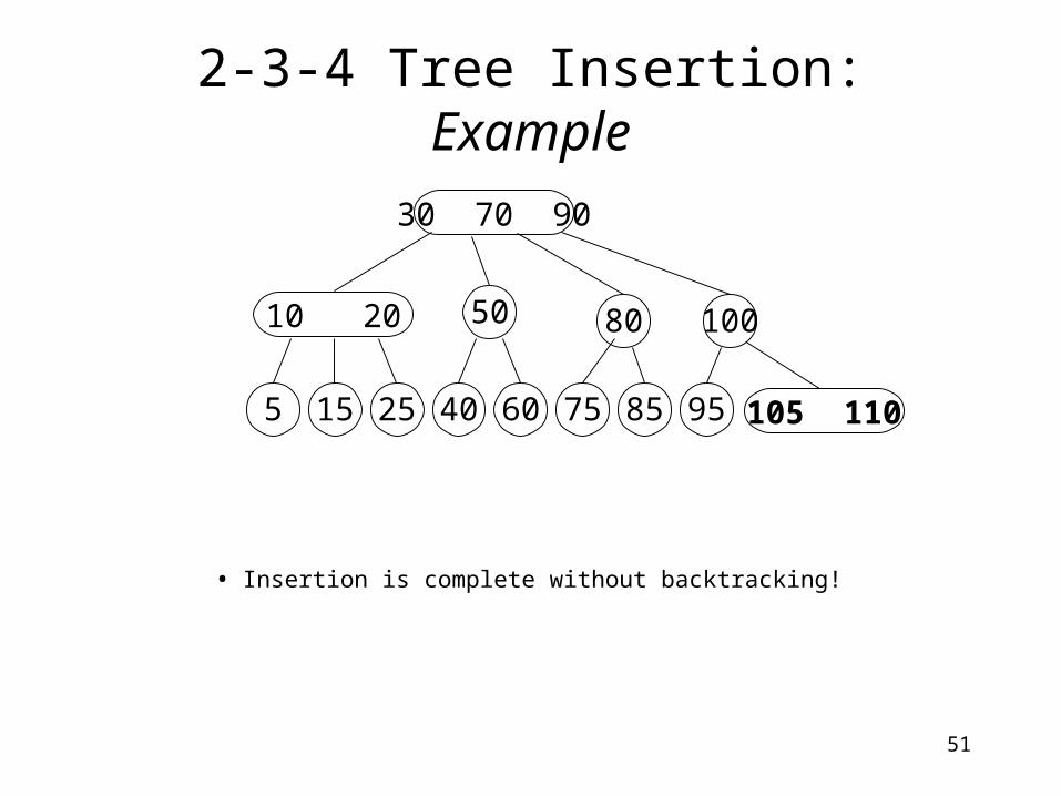
2-3-4 Tree Insertion: Example
• Since 105 > 90, search for the leaf into which 105 can be inserted continues with node n2.
• The leaf containing 110 is found and, since it contains only one item, 105 is inserted.
10 20
11095
p
10050 80
30 70 90
255 15 75 8540 60
n1 n2
51
2-3-4 Tree Insertion: Example
• Insertion is complete without backtracking!
10 20
95
10050 80
30 70 90
255 15 75 8540 60 105 110

52
Red-Black Tree
• 2-3 trees have an advantage over binary search trees, since they are always balanced.
• 2-3-4 trees have an advantage over 2-3 trees, since, in addition to being always balanced, insertion and deletion require only one pass from the root to a leaf.
• However, 2-3-4 trees require more storage than 2-3 trees due to the fact that each node must carry space for 3 items, regardless of how many items are actually stored.
• Red-black trees address this issue by representing 2-3-4 trees as binary search trees, thereby only allocating space for existing data items.

53
Red-Black Tree
• Let all child pointers in the original 2-3-4 tree be black.
• Use red child pointers to link the 2-nodes that result when 3-nodes and 4-nodes are split to form binary tree nodes.
S M L
a b c d
S L
a b cS
L
a b
c
M
LS
a b c d
L
S
b c
aor

54
Red-Black Tree: Example30 70
255 15 75 11085 95
10 20
40 60
50 80 90 100
2-3-4 tree
75 11085 95
40 60
50
70
30
80 100
9025
20
10
5 15
corresponding red-black tree

55
Red-Black Tree: Observations
• Since a red-black tree is a binary search tree, you can use the binary search tree algorithms to search and traverse it. (Ignore the color of the pointers.)
• Since a red-black tree represents a 2-3-4 tree, the 2-3-4 tree algorithms can be used to insert and delete items.
• The primary open issue is how to split a node in a 2-3-4 tree when it is implemented as a red-black tree. This process is illustrated on the following viewgraphs.
56
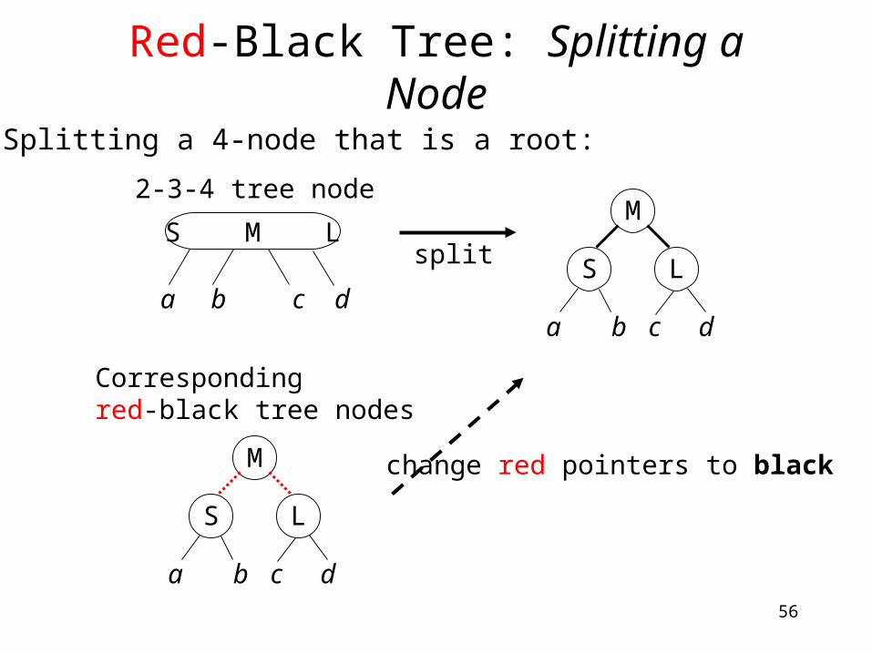
Red-Black Tree: Splitting a Node
1. Splitting a 4-node that is a root:
S M L
a b c d
M
LS
a b c d
2-3-4 tree node
Correspondingred-black tree nodes
M
LS
a b c d
split
change red pointers to black

57
Red-Black Tree: Splitting a Node (Cont’d.)
2. Splitting a 4-node with a 2-node parent:
correspondingred-black tree nodes
split
change colorof pointersM
LS
a b c d
P
e
2-3-4tree nodes
a b c d
S M L
P
e LS
a b c d
M P
e
M
LS
a b c d
P
e

58
Red-Black Tree: Splitting a Node (Cont’d.)
3. Splitting a 4-node with a 3-node parent:
correspondingred-black tree nodes
split2-3-4tree nodes
a b c d
S M L e f
P Q
M
LS
a b c d
P
e
Q
f
a b c d
e fS L
M P Q
M
LS
a b c d
e
Q
f
P
rotate and changecolor of pointers

59
Red-Black Tree: Summary
• Since red-black trees are always balanced, searching, inserting, and deleting an item from a tree of n nodes is never worse than O( log n ).
• Since inserting and deleting an item in a red-black tree frequently requires only changing the color of pointers, these operations are more time-efficient in a red-black tree than in the corresponding 2-3-4 tree.
• Finally, since it is unnecessary to reserve extra space in the nodes of a red-black tree to accommodate potential, future items, red-black trees are more space-efficient than either 2-3 trees or 2-3-4 trees.

60
AVL Tree• The AVL Tree is named after its inventors, G. M. Adel’son-
Vel’skii and E. M. Landis, and refers to one of the oldest methods for maintaining a balanced, binary tree.
• An AVL tree is a balanced, binary search tree in which:
– insertions and deletions are done as in a typical, binary search tree; however,
– after each insertion or deletion, a check is done to determine whether any node in the tree has left and right subtrees with heights that differ by > 1;
– if so, the nodes in the tree are rearranged to restore its balance.
• The process of restoring the balance to an AVL tree is called a rotation.

61
AVL Tree: Restoring Balance
20
10 40
30
25
50
60
Unbalancedbinary search tree
40
20
10 30
50
60
25
Balanced treeafter one left rotation
deleted edge new edge
62
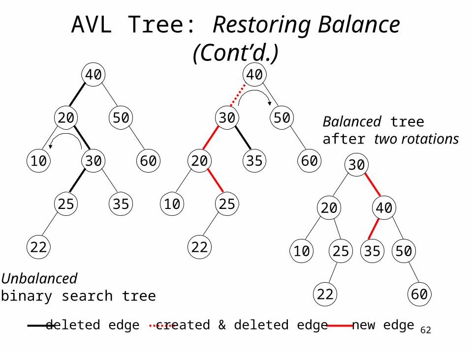
AVL Tree: Restoring Balance (Cont’d.)
deleted edge new edge
Unbalancedbinary search tree
Balanced treeafter two rotations
20
10 30
25
22
35
40
50
60
30
20
10 25
35
22
40
50
60 30
10 25
22 60
35 50
4020
created & deleted edge

63
AVL Tree: Remarks
• The height of an AVL tree with n nodes will always be close to the theoretical minimum of log2 (n + 1) .
• Consequently, search, insertion and deletion can all be done efficiently as O( log n ) operations.
• Also, no extra space needs to be reserved in each node for potential, future items, as in a 2-3 tree or 2-3-4 tree.
• However, implementation of a 2-3-4 tree or a red-black tree will usually be simpler than the implementation of an AVL tree.
64
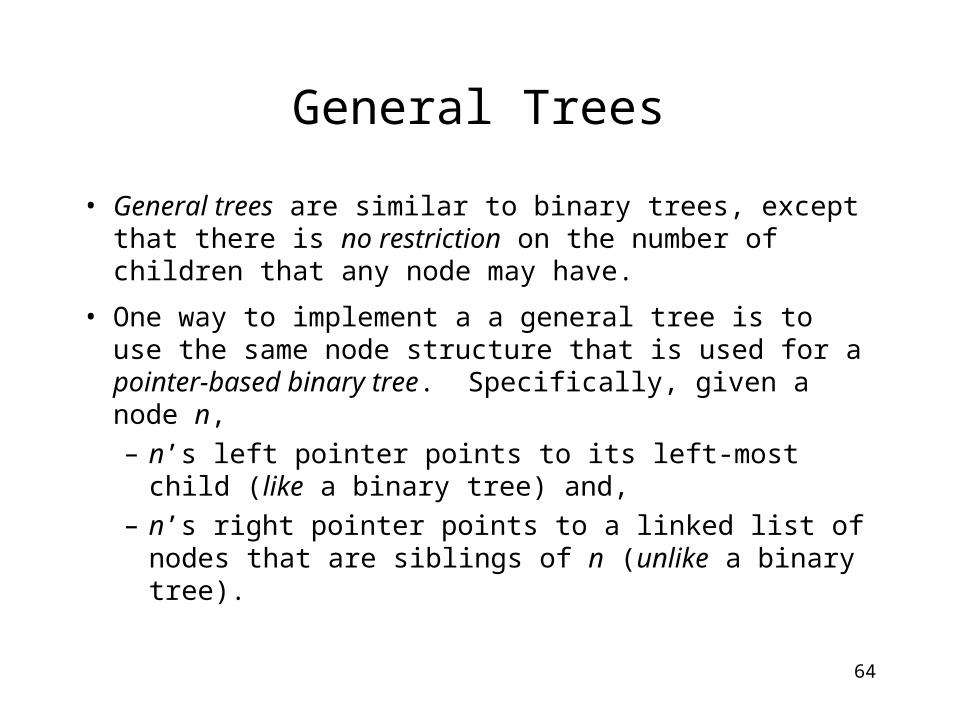
General Trees
• General trees are similar to binary trees, except that there is no restriction on the number of children that any node may have.
• One way to implement a a general tree is to use the same node structure that is used for a pointer-based binary tree. Specifically, given a node n,
– n’s left pointer points to its left-most child (like a binary tree) and,
– n’s right pointer points to a linked list of nodes that are siblings of n (unlike a binary tree).

65
General Trees: Example
Pointer-based implementation of the general tree
B
A
E F G H I
DC
A
HF GE I
B C D
A general tree

66
General Trees: Example (Cont’d.)
B
A
E F G H I
DC
A
F
G
E
H
B
C
D
I
Binary tree withthe pointer structureof the precedinggeneral tree

67
N-ary Trees
• An n-ary tree is a generalization of a binary tree, where each node can have no more than n children.
• Since the maximum number of children for any node is known, each parent node can point directly to each of its children -- rather than requiring a linked list.
• This results in a faster search time (if you know which child you want).
• The disadvantage of this approach is that extra space reserved in each node for n child pointers, many of which may not be used.
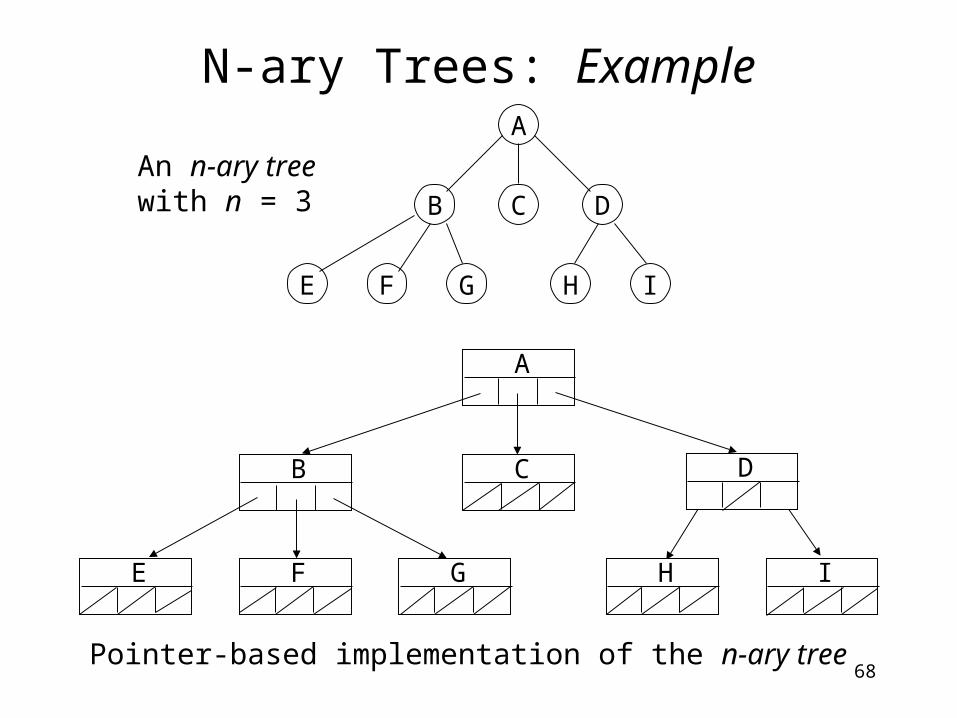
68
N-ary Trees: ExampleA
HF GE I
B C D
An n-ary treewith n = 3
Pointer-based implementation of the n-ary tree
A
B
E F G H I
C D