1

Artificial Neural Networks

Inputlayer

Firsthiddenlayer

Secondhiddenlayer

Outputlayer

O u

t p

u t

S

i g n

a l

s

I n

p u

t S

i g

n a

l s

2

Commercial ANNs

• Commercial ANNs incorporate three and Commercial ANNs incorporate three and sometimes four layers, including one or two sometimes four layers, including one or two hidden layers. Each layer can contain from hidden layers. Each layer can contain from 10 to 1000 neurons. Experimental neural 10 to 1000 neurons. Experimental neural networks may have five or even six layers, networks may have five or even six layers, including three or four hidden layers, and including three or four hidden layers, and utilise millions of neurons.utilise millions of neurons.

Example

• Character recognition

3

Problems that are not linearly separable

• Xor function is not linearly separable

• Using Multilayer networks with back propagation training algorithm

• There are hundreds of training algorithms for multilayer neural networks

4

5

Multilayer neural networksMultilayer neural networks

A multilayer perceptron is a feedforward neural A multilayer perceptron is a feedforward neural network with one or more hidden layers. network with one or more hidden layers.

The network consists of an The network consists of an input layerinput layer of source of source neurons, at least one middle or neurons, at least one middle or hidden layerhidden layer of of computational neurons, and an computational neurons, and an output layeroutput layer of of computational neurons. computational neurons.

The input signals are propagated in a forward The input signals are propagated in a forward direction on a layer-by-layer basis.direction on a layer-by-layer basis.

6

Multilayer perceptron with two hidden layersMultilayer perceptron with two hidden layers

Inputlayer

Firsthiddenlayer

Secondhiddenlayer

Outputlayer

O u

t p

u t

S

i g n

a l

s

I n

p u

t S

i g

n a

l s

7

What do the middle layers hide?What do the middle layers hide?

A hidden layer “hides” its desired output. Neurons A hidden layer “hides” its desired output. Neurons in the hidden layer cannot be observed through the in the hidden layer cannot be observed through the input/output behaviour of the network. There is no input/output behaviour of the network. There is no obvious way to know what the desired output of the obvious way to know what the desired output of the hidden layer should be. hidden layer should be.

8

Back-propagation neural networkBack-propagation neural network

Learning in a multilayer network proceeds the Learning in a multilayer network proceeds the same way as for a perceptron. same way as for a perceptron.

A training set of input patterns is presented to the A training set of input patterns is presented to the network. network.

The network computes its output pattern, and if The network computes its output pattern, and if there is an error there is an error or in other words a difference or in other words a difference between actual and desired output patterns between actual and desired output patterns the the weights are adjusted to reduce this error.weights are adjusted to reduce this error.

9

In a back-propagation neural network, the learning In a back-propagation neural network, the learning algorithm has two phases. algorithm has two phases.

First, a training input pattern is presented to the First, a training input pattern is presented to the network input layer. The network propagates the network input layer. The network propagates the input pattern from layer to layer until the output input pattern from layer to layer until the output pattern is generated by the output layer. pattern is generated by the output layer.

If this pattern is different from the desired output, If this pattern is different from the desired output, an error is calculated and then propagated an error is calculated and then propagated backwards through the network from the output backwards through the network from the output layer to the input layer. The weights are modified layer to the input layer. The weights are modified as the error is propagated.as the error is propagated.

10

Three-layer back-propagation neural networkThree-layer back-propagation neural network

Inputlayer

xi

x1

x2

xn

1

2

i

n

Outputlayer

1

2

k

l

yk

y1

y2

yl

Input signals

Error signals

wjk

Hiddenlayer

wij

1

2

j

m

11

Step 1Step 1: Initialisation: InitialisationSet all the weights and threshold levels of the Set all the weights and threshold levels of the network to random numbers uniformly network to random numbers uniformly distributed inside a small range:distributed inside a small range:

where where FFii is the total number of inputs of neuron is the total number of inputs of neuron ii

in the network. The weight initialisation is done in the network. The weight initialisation is done on a neuron-by-neuron basis.on a neuron-by-neuron basis.

The back-propagation training algorithmThe back-propagation training algorithm

ii FF

4.2 ,

4.2

12

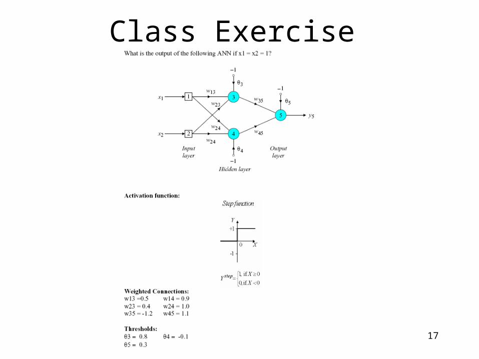
Three-layer networkThree-layer network

y55

x1 31

x2

Inputlayer

Outputlayer

Hidden layer

42

3

w13

w24

w23

w24

w35

w45

4

5

1

1

1

ww13 = 0.5, 13 = 0.5, ww14 = 0.9, 14 = 0.9, ww23 = 0.4, 23 = 0.4, ww24 = 1.0, 24 = 1.0, ww35 = 35 = 1.2, 1.2, ww45 = 1.1, 45 = 1.1, 3 = 0.8, 3 = 0.8, 4 = 4 = 0.1 and 0.1 and 5 = 0.3 5 = 0.3

13

The effect of the threshold applied to a neuron in the The effect of the threshold applied to a neuron in the hidden or output layer is represented by its weight, hidden or output layer is represented by its weight, , , connected to a fixed input equal to connected to a fixed input equal to 1.1.

The initial weights and threshold levels are set The initial weights and threshold levels are set randomly e.g., as follows:randomly e.g., as follows:ww1313 = 0.5, = 0.5, ww1414 = 0.9, = 0.9, ww2323 = 0.4, = 0.4, ww2424 = 1.0, = 1.0, ww3535 = = 1.2, 1.2,

ww4545 = 1.1, = 1.1, 33 = 0.8, = 0.8, 44 = = 0.1 and 0.1 and 55 = 0.3. = 0.3.

14

Assuming the sigmoid activation Function

15

Step 2Step 2: Activation: ActivationActivate the back-propagation neural network by Activate the back-propagation neural network by applying inputs applying inputs xx11((pp), ), xx22((pp),…, ),…, xxnn((pp) and desired ) and desired

outputs outputs yydd,1,1((pp), ), yydd,2,2((pp),…, ),…, yydd,,nn((pp).).

((aa) Calculate the actual outputs of the neurons in ) Calculate the actual outputs of the neurons in the hidden layer:the hidden layer:

where where nn is the number of inputs of neuron is the number of inputs of neuron jj in the in the hidden layer, and hidden layer, and sigmoidsigmoid is the is the sigmoidsigmoid activation activation function.function.

j

n

iijij pwpxsigmoidpy

1

)()()(

16

((bb) Calculate the actual outputs of the neurons in ) Calculate the actual outputs of the neurons in the output layer:the output layer:

where where mm is the number of inputs of neuron is the number of inputs of neuron kk in the in the output layer.output layer.

k

m

jjkjkk pwpxsigmoidpy

1

)()()(

Step 2Step 2: Activation (continued): Activation (continued)

17

Class Exercise

18

If the sigmoid activation function is used the output of If the sigmoid activation function is used the output of the hidden layer isthe hidden layer is

5250.01 /1)( )8.014.015.01(32321313 ewxwx sigmoidy

8808.01 /1)( )1.010.119.01(42421414 ewxwx sigmoidy

And the actual output of neuron 5 in the output layer isAnd the actual output of neuron 5 in the output layer is

And the error isAnd the error is

5097.01 /1)( )3.011.18808.02.15250.0(54543535 ewywy sigmoidy

5097.05097.0055, yye d

19

What learning law applies in a multilayer neural network?

)()()( ppypw kjjk

20

Step 3Step 3: Weight training output layer: Weight training output layerUpdate the weights in the back-propagation network Update the weights in the back-propagation network propagating backward the errors associated with propagating backward the errors associated with output neurons.output neurons.((aa) Calculate the error) Calculate the error

and then the error gradient for the neurons in the and then the error gradient for the neurons in the output layer:output layer:

Then the weight corrections:Then the weight corrections:

Then the new weights at the output neurons:Then the new weights at the output neurons:

)()(1)()( pepypyp kkkk

)()()( , pypype kkdk

)()()( ppypw kjjk

)()()1( pwpwpw jkjkjk

21

Three-layer network for solving the Three-layer network for solving the Exclusive-OR operationExclusive-OR operation

y55

x1 31

x2

Inputlayer

Outputlayer

Hidden layer

42

3

w13

w24

w23

w24

w35

w45

4

5

1

1

1

22

The error gradient for neuron 5 in the output layer:The error gradient for neuron 5 in the output layer:

1274.05097).0( 0.5097)(1 0.5097)1( 555 e y y

Determine the weight corrections assuming that the Determine the weight corrections assuming that the learning rate parameter, learning rate parameter, , is equal to 0.1:, is equal to 0.1:

0112.0)1274.0(8808.01.05445 yw0067.0)1274.0(5250.01.05335 yw

0127.0)1274.0()1(1.0)1( 55

Apportioning error inthe hidden layer

• Error is apportioned in proportion to the weights of the connecting arcs.

• Higher weight indicates higher error responsibility

23

24

((bb) Calculate the error gradient for the neurons in ) Calculate the error gradient for the neurons in the hidden layer:the hidden layer:

Calculate the weight corrections:Calculate the weight corrections:

Update the weights at the hidden neurons:Update the weights at the hidden neurons:

)()()(1)()(1

][ p wppypyp jk

l

kkjjj

)()()( ppxpw jiij

)()()1( pwpwpw ijijij

Step 3Step 3: Weight training hidden layer: Weight training hidden layer

25

The error gradients for neurons 3 and 4 in the hidden The error gradients for neurons 3 and 4 in the hidden layer:layer:

Determine the weight corrections:Determine the weight corrections:

0381.0)2.1 (0.1274) (0.5250)(1 0.5250)1( 355333 wyy

0.0147.11 4) 0.127 ( 0.8808)(10.8808)1( 455444 wyy

0038.00381.011.03113 xw0038.00381.011.03223 xw

0038.00381.0)1(1.0)1( 33 0015.0)0147.0(11.04114 xw0015.0)0147.0(11.04224 xw

0015.0)0147.0()1(1.0)1( 44

26

At last, we update all weights and threshold:At last, we update all weights and threshold:

5038.00038.05.0131313 www

8985.00015.09.0141414 www

4038.00038.04.0232323 www

9985.00015.00.1242424 www

2067.10067.02.1353535 www

0888.10112.01.1454545 www

7962.00038.08.0333

0985.00015.01.0444

3127.00127.03.0555

The training process is repeated until the sum of The training process is repeated until the sum of squared errors is less than 0.001. squared errors is less than 0.001.

27

Step 4Step 4: Iteration: IterationIncrease iteration Increase iteration pp by one, go back to by one, go back to Step 2Step 2 and and repeat the process until the selected error criterion repeat the process until the selected error criterion is satisfied.is satisfied.

As an example, we may consider the three-layer As an example, we may consider the three-layer back-propagation network. Suppose that the back-propagation network. Suppose that the network is required to perform logical operation network is required to perform logical operation Exclusive-ORExclusive-OR. Recall that a single-layer perceptron . Recall that a single-layer perceptron could not do this operation. Now we will apply the could not do this operation. Now we will apply the three-layer net.three-layer net.

28

Typical Learning CurveTypical Learning Curve

0 50 100 150 200

101

Epoch

Su

m-S

qu

are

d E

rro

rSum-Squared Network Error for 224 Epochs

100

10-1

10-2

10-3

10-4

29

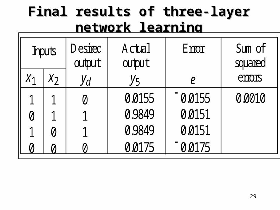
Final results of three-layer network learningFinal results of three-layer network learning

Inputs

x1 x2

1010

1100

011

Desiredoutput

yd

0

0.0155

Actualoutput

y5Y

Error

e

Sum ofsquarederrors

e 0.9849 0.9849 0.0175

0.0155 0.0151 0.0151 0.0175

0.0010

30

Network represented by McCulloch-Pitts model Network represented by McCulloch-Pitts model for solving the for solving the Exclusive-ORExclusive-OR operation operation

y55

x1 31

x2 42

+1.0

1

1

1+1.0

+1.0

+1.0

+1.5

+1.0

+1.0

+0.5

+0.5

31

Accelerated learning in multilayer Accelerated learning in multilayer neural networksneural networks

A multilayer network learns much faster when the A multilayer network learns much faster when the sigmoidal activation function is represented by a sigmoidal activation function is represented by a hyperbolic tangenthyperbolic tangent::

where where aa and and bb are constants. are constants.

Suitable values for Suitable values for aa and and bb are: are: aa = 1.716 and = 1.716 and bb = 0.667 = 0.667

ae

aY

bXhtan

1

2

32

We also can accelerate training by including a We also can accelerate training by including a momentum termmomentum term in the delta rule: in the delta rule:

where where is a positive number (0 is a positive number (0 1) called the 1) called the momentum constantmomentum constant. Typically, the momentum . Typically, the momentum constant is set to 0.95.constant is set to 0.95.

This equation is called the This equation is called the generalised delta rulegeneralised delta rule..

)()()1()( ppypwpw kjjkjk

33

Learning with an adaptive learning rateLearning with an adaptive learning rate

To accelerate the convergence and yet avoid the To accelerate the convergence and yet avoid the

danger of instability, we can apply two heuristics:danger of instability, we can apply two heuristics:

HeuristicHeuristicIf the error is decreasing the learning rate If the error is decreasing the learning rate , should be , should be increased.increased.

If the error is increasing or remaining constant the If the error is increasing or remaining constant the learning rate learning rate , should be decreased., should be decreased.

34

Adapting the learning rate requires some changes Adapting the learning rate requires some changes in the back-propagation algorithm. in the back-propagation algorithm.

If the sum of squared errors at the current epoch If the sum of squared errors at the current epoch exceeds the previous value by more than a exceeds the previous value by more than a predefined ratio (typically 1.04), the learning rate predefined ratio (typically 1.04), the learning rate parameter is decreased (typically by multiplying parameter is decreased (typically by multiplying by 0.7) and new weights and thresholds are by 0.7) and new weights and thresholds are calculated. calculated.

If the error is less than the previous one, the If the error is less than the previous one, the learning rate is increased (typically by multiplying learning rate is increased (typically by multiplying by 1.05).by 1.05).

35

Typical Learning CurveTypical Learning Curve

0 50 100 150 200

101

Epoch

Su

m-S

qu

are

d E

rro

rSum-Squared Network Error for 224 Epochs

100

10-1

10-2

10-3

10-4

36

Typical learning with adaptive learning rateTypical learning with adaptive learning rate

0 10 20 30 40 50 60 70 80 90 100Epoch

Training for 103 Epochs

0 20 40 60 80 100 1200

0.2

0.4

0.6

0.8

1

Epoch

Le

arn

ing

Ra

te

10-4

10-2

100

102S

um

-Sq

ua

red

Err

or

10-3

101

10-1

37

Typical Learning with Typical Learning with adaptive learning rate plus momentumadaptive learning rate plus momentum

0 10 20 30 40 50 60 70 80Epoch

Training for 85 Epochs

0 10 20 30 40 50 60 70 80 900

0.5

1

2.5

Epoch

Lea

rnin

g R

ate

10-4

10-2

100

102

Su

m-S

qu

are

d E

rro

r

10-3

101

10-1

1.5

2