1 analysis of snowpack properties and structure from ... · recently launched high precision...

1

Analysis of snowpack properties and structure

from TerraSAR-X data, based on multilayer

backscattering and snow evolution modeling

approaches

Xuan-Vu Phan, Laurent Ferro-Famil, Member, IEEE, Michel Gay, Member, IEEE,

Yves Durand, Marie Dumont, Sophie Allain and Guy D’Urso

Abstract

Recently launched high precision Synthetic Aperture Radar (SAR) satellites such as TerraSAR-

X, COSMO-SkyMed, etc. present a high potential for better observation and characterization of the

cryosphere. This study introduces a new approach using high frequency (X-band) SAR data and an

Electromagnetic Backscattering Model (EBM) to constrain the detailed snowpack model Crocus. A

snowpack EBM based on radiative transfer theory, previously used for C-band applications, is adapted

for the X-band. From measured or simulated snowpack stratigraphic profiles consisting of snow optical

grain radius and density, this forward model calculates the backscattering coefficient σ0 for different

polarimetric channels. The output result is then compared with spaceborne TerraSAR-X acquisitions

to evaluate the forward model. Next, from the EBM, the adjoint operator is developed and used in

a variational analysis scheme in order to minimize the discrepancies between simulations and SAR

observations. A time series of TerraSAR-X acquisitions and in-situ measurements on the Argentiere

glacier (Mont-Blanc massif, French Alps) are used to evaluate the EBM and the data assimilation

scheme. Results indicate that snow stratigraphic profiles obtained after the analysis process show a

Xuan-Vu Phan and Michel Gay are with the Grenoble Image Parole Signal et Automatique lab, Grenoble, France.

Laurent Ferro-Famil and Sophie Allain are with the Institut d’Electronique et de Telecommunications de Rennes, University

of Rennes, France.

Yves Durand and Marie Dumont is with Meteo-France and CNRS, CNRM-GAME, URA-1357, Centre d’Etude de la Neige,

France.

Guy D’Urso is with Electricite de France, Paris, France.

November 15, 2012 DRAFT

arX

iv:1

211.

3278

v1 [

phys

ics.

com

p-ph

] 1

4 N

ov 2

012

2

closer agreement with the measured ones than the initial ones, and therefore demonstrate the high

potential of assimilating SAR data to model of snow evolution.

Index Terms

Remote sensing, electromagnetic backscattering model, snow grain size, snow density, radar (SAR),

data analysis.

I. INTRODUCTION

Snowpack characterization has become a critical issue in the present context of climate change.

Estimating some of the properties of a snowpack, like its density and grain size distribution

will provide great benefit to snow forecasting, prevision of natural hazard, like snow avalanche

warning, and economic arrangements related to tourism and winter sports. Due to its imaging

capabilities over large areas, unaffected by weather and day-night conditions, Synthetic Aperture

Radar (SAR) is an important tool for snowpack characterization in a natural environment.

Moreover, the high penetration depth of radar electromagnetic waves allow us to retrieve the

information inside the volume of the snowpack. Over the past decade, the large availability of

L and C-band SAR data provided by various spaceborne sensors, like ALOS PALSAR, ERS-1,

ENVISAT, led to many studies on the characterization of snowpack properties [1], [2].

A new generation of X-band (8-12GHz) SAR systems, and in the near future Ku-band (12-

18GHz), with high image resolution, short revisit time will provide improved information that

might be used to characterize and monitor snowpack. In this context, it is necessary to develop

a compatible EBM accounting for electromagnetic waves (EMW) propagation and scattering at

high frequencies (X and Ku-bands) through a multilayer snowpack. Some backscattering models

at L and C-band frequencies have been introduced in [2], [3]. These models simulate the loss

of EMW energy while propagating through dense media by solving the Radiative Transfer (RT)

differential equation [4]. In order to introduce coherent recombination effects in the RT coherent

model, Wang. et al. [5] applied the Strong Fluctuation Theory (SFT) introduced by Stogryn [6] to

calculate the effective permittivity of each snow layer, in which the correlation among particles

was taken into account. The scattering and absorption mechanisms in the EBM are simulated

using the Rayleigh scattering model due to the snow grain size being in this study is much

smaller than the carrier wavelength.


3

In this paper, the snowpack backscattering model initially developed in [2] is adapted for

X-band and higher frequencies, in the case of a dry snow medium. The adaptation consists of

updating the IEM introduced by Fung et. al. in 1992 [7] by a newer version published in 2004 [8],

which allows the calculation of surface and ground backscattering components for X-band and

higher frequencies. Meanwhile the modeling of volume backscattering of the existed model,

which is based on solving the Vector Radiative Transfer equation and Rayleigh scattering model,

is compatible for X and Ku-bands. From the physical features of each snow layer (optical grain

radius, density, thickness) and for given SAR acquisition conditions (frequency, incidence angle),

the model calculates the total backscattering coefficient σ0pq for different polarization channels

and their vertical distribution within the snowpack. Next, the snowpack profiles generated by

the detailed snowpack model Crocus using downscaled meteorological fields from the SAFRAN

analysis [9]–[11], are constrained using the SAR image data and EBM simulations. In this study,

the number of observable, i.e. the SAR backscattering coefficients, being much smaller than the

number of unknown parameters, i.e. the snow cover properties, a classical estimation approach

based on the use of an inverse problem would reveal totally inefficient. Instead, an adjoint operator

of the direct EBM is developed to be used in a assimilation scheme. A variational assimilation

method allows the integration of the observation data into a set of initial guess parameters

through a direct model, and therefore can constrain these parameters without explicitly inverting

the model. In our study, the three-dimensional variational analysis (3D-VAR) method [12] is

implemented. Finally, a time series of TerraSAR-X acquisitions on the mountainous region of

the French-Alps is used to evaluate the model and the data assimilation process. The Argentiere

glacier area has been chosen for the case study due to its large, uniformly snow-covered surface

area. Some in-situ measurements on this area are also available at the same timeline of SAR

acquisitions and therefore are used to evaluate the EBM and the performance of the data

assimilation scheme.

Details of the EBM equations and its the physical and mathematical hypothesis are presented

in section II. An introduction to the Crocus detailed snowpack model and to the detailed imple-

mentation of the 3D-VAR scheme are described in section III. Section IV shows a description

of TerraSAR-X acquisition parameters, as well as results of the case study on the Argentiere

glacier.


4

Fig. 1. Main backscattering mechanisms occurring within a multilayer snowpack that can be simulated using the RT theory at

order 1: air-snow reflection (Mas), volume scattering (Mvol) and reflection over the ground (Mg).

II. EMW BACKSCATTERING MODEL

A. Main components of the total backscattering coefficient

The Stoke vector, which contains the incoherent information related to the polarization of an

electromagnetic wave, can be expressed as:

g =

⟨|Eh|2

⟩+⟨|Ev|2

⟩⟨|Eh|2

⟩−⟨|Ev|2

⟩2<e 〈EhE∗v〉

−2=m 〈EhE∗v〉

(1)

where Eh and Ev represent the horizontal and vertical components of the Jones vector on the

electric field [13], and 〈.〉 represents the expectation operator.

For given acquisition conditions, the Stoke vector scattered by a medium, gs, can be related

to the incident one, gi, by a Mueller matrix M as gs = Mgi with:

M =

M11 0 0 0

0 M22 0 0

0 0 M33 M34

0 0 −M34 M33

(2)


5

where M11 = σ0vv and M22 = σ0

hh represent the co-polarized backscattering coefficients and

M33 = <e(σ0vvhh) and M34 = =m(σ0

vvhh) are correlation terms. Due to the reflection symmetry,

the cross-polarization coefficients of the matrix σpppq are equal to zero [13], and the rest of the

elements of M are null.

The solution of the RT equation at order 1 provides a total backscattered information from

a snowpack that consists of a combination of five scattering mechanisms: reflection at the

surface air-snow interface, volume scattering, volume-ground and ground-volume interactions,

and reflection over the ground [14]. Due to their small amplitude, the volume-ground and ground-

volume contributions can be neglected [15]. The illustration of the three other mechanisms is

shown in Fig. 1. The expression of the total polarimetric backscattered information can be written

using the Mueller matrix corresponding to each mechanism:

Msnow = Mas + Mvol + Mg (3)

The surface and ground backscattering are modeled using the IEM introduced by Fung

et. al. [8], whereas the volume contribution is calculated using the Vector Radiative Transfer

equation.

B. Surface backscattering

The matrix Mas represents the second order polarimetric response backscattered by the air-

snow interface. Its elements can be calculated from the surface roughness parameters, e.g. its

correlation function w(x) and its root mean square (rms) height σh, the incidence angle θ0 and

the emitted EM wave frequency f using the Integration Equation Model (IEM) [8]. According

to the IEM, the reflectivity may be expressed as:

σ0pq =

k20

4πexp(−2k2

0σ2h cos2 θ0)

∞∑n=1

|Inpq|2W n(2k0 sin θ0, 0)

n!(4)

where p and q are equal to h or v, indicating a horizontal or vertical polarization, k0 = 2πfc

represents the wave number. The detailed mathematical expressions of the surface spectrum W n

and the Fresnel reflection/transmission factor |Inpq| can be found in [8].

C. Volume backscattering

The volume backscattering Mvol is deduced from the loss of EMW intensity during propagation

through a multilayer snowpack, which can be categorized into 4 types: related to transmission


6

between two layers, absorption by the snow particles, scattering and coherent recombination.

The amplitude of each mechanism depends largely on the dielectric properties of the snowpack

medium. Therefore the permittivity of each layer, which characterizes its dielectric properties,

needs to be calculated first:

1) Dry snow permittivity: Dry snow is considered as a dense and heterogeneous medium

with strong variations of various physical properties such as grain size, density, thickness.

Therefore the variance of permittivity across a snow layer is relatively high. Several snowpack

characterization methods [16] are largely based on the assumption that the scattering losses due

to the correlation of EMW are negligible. However, at high frequency, the snowpack structure

becomes bigger compared to the wavelength of X or Ku-band EM waves [17]. The correlation

between particles can no longer be ignored. The Strong Fluctuation Theory (SFT) introduced

by Stogryn [6] can model the permittivity of such medium by using the effective permittivity

(εeff ) that takes into account the scattering effect among ice particles at high frequencies. The

expression of εeff using SFT is as follows [17]:

εeff = εg + j.4

3δεg .k

30.√εg.L

3 (5)

where εg and δεg are the quasi-static permittivity and its variance, k0 the wave number and L the

correlation length, which is proportional to the average snow grain size and the snow density of

the medium.

2) Transmission between two layers: The snowpack consists of layers with different physical

properties. Therefore the model needs to take into account the energy loss due to transmission

between two layers. With the assumption of a smooth interface between two layers, the Fresnel

transmission can be used. It is expressed through a matrix as follows [4]:

Tk(k−1) =εk−1

εk

∣∣∣tvvk(k−1)

∣∣∣2 0 0 0

0∣∣∣thhk(k−1)

∣∣∣2 0 0

0 0 gk(k−1) −hk(k−1)

0 0 hk(k−1) gk(k−1)

(6)


7

where∣∣∣tppk(k−1)

∣∣∣2 represents the Fresnel transmission coefficients of pp channel, whereas gk(k−1)

and hk(k−1) are the terms of Mueller matrix related to the co-polarized correlation [2]:

gk(k−1) =cos θk−1

cos θk<e(tvvk(k−1)t

hh∗k(k−1)) and hk(k−1) =

cos θk−1

cos θk=m(tvvk(k−1)t

hh∗k(k−1)) (7)

3) The attenuation: The particles in a snowpack are generally considered as spheres [3], [15],

[18]. Due to the spherical symmetry of the particle shape, the extinction of a wave propagating

through the snowpack is independent of the polarization and may hence be represented by a

scalar coefficient. The extinction is composed of an absorption and a scattering terms:

κe = κa + κs (8)

It can also be computed through the effective permitivity εeff [17]:

κe = 2k0Im∣∣∣√εeff ∣∣∣ (9)

The attenuation matrix represents the gradual loss in EMW intensity while penetrating through

a multilayer snowpack, composed of layers with different physical properties. It takes into account

the energy loss by absorption and scattering mechanisms based on the extinction coefficient κe

and thickness d of the layer, as well as the loss by transmission effect while an EM propagate

through different layers:

Attdown(k) =k∏i=1

exp(− κied

i

cos θi

)Ti(i−1) (10)

Attup(k) =k∏i=1

T(i−1)i exp(− κied

i

cos θi

)(11)

The Attdown is the intensity loss when propagating from the surface to layer k, whereas Attuprepresents the intensity loss from layer k to the surface. The exponential factor, which takes

into account the gradual loss of energy throughout the layer, is deduced from the basic radiative

transfer equation dI = Iκedr where r = d/cosθ.

4) Scattering by the particles: The phase matrix Pk under the hypothesis of spherical particles

has the form shown in (2) where the cross-polarization terms P12 and P21 are null. In the

backscattering case, with the assumption of spherical particles, the SFT phase matrix can be

simplified to Pk = 3κs8πI4 where I4 is the (4x4) identity matrix [19].


8

5) Calculation of the volume backscattering: If we consider a snowpack made of n distinct

layers, where θk is the incidence angle and dk is the thickness of layer k, the total contribution

of the volume backscattering mechanism Mvol can be written as follows:

Mvol = 4π cos θ0

n∑k=1

Attup(k − 1)T(k−1)k

.1− exp

(−2κked

k

cos θk

)2κke

PkTk(k−1)Attdown(k − 1) (12)

D. Ground backscattering

The backscattering Mg of the snow-ground interface may be computed as:

Mg = cos θ0 Attup(n)R(θn)

cos θnAttdown(n) (13)

where R(θn) represents the contribution of the underlying ground surface backscattering and can

be determined using the IEM.

III. 3D-VAR DATA ASSIMILATION

A. The detailed snowpack model Crocus

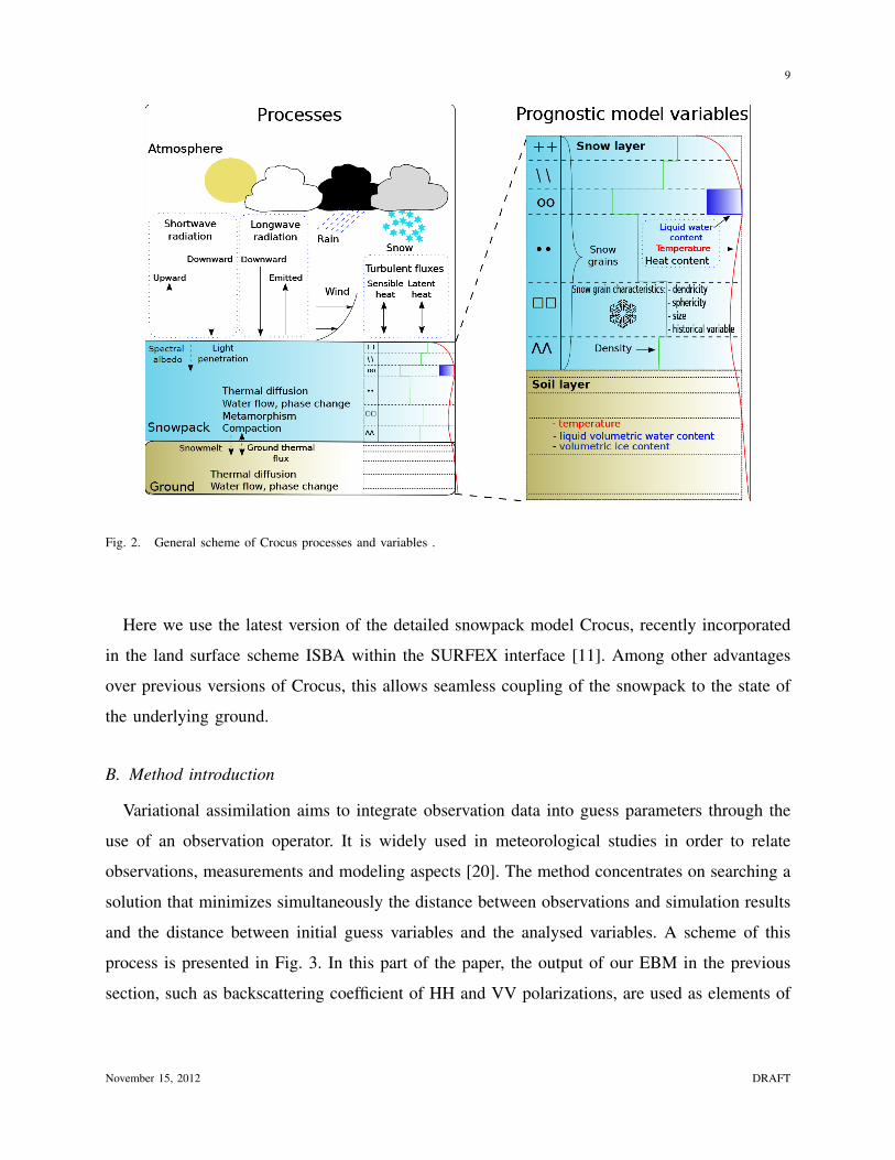
Crocus is a one-dimensional numerical model simulating the thermodynamic balance of energy

and mass of the snowpack. Its main objective is to describe in detail the evolution of internal

snowpack properties based on the description of the evolution of morphological properties of

snow grains during their metamorphism. Fig. 2 describes the general scheme of Crocus. It takes

as input the meteorological variables air temperature, relative air humidity, wind speed, solar

radiation, long wave radiation, amount and phase of precipitation. When it is used in the French

mountain ranges (Alps, Pyrenees and Corsica), these quantities are commonly provided by the

SAFRAN system, which combines ground-based and radiosondes observations with an a priori

estimate of meteorological conditions from a numerical weather prediction (NWP) model [9],

[10]. The output includes the scalar physical properties of the snowpack (snow depth, snow

water equivalent, surface temperature, albedo, . . . ) along with the internal physical properties

for each layer (density, thickness, optical grain radius, . . . ). SAFRAN meteorological fields are

assumed to be homogeneous within a given mountrain range and provide a description of the

altitude dependency of meteorological variables by steps of 300 m elevation [9], [10].


9

Fig. 2. General scheme of Crocus processes and variables .

Here we use the latest version of the detailed snowpack model Crocus, recently incorporated

in the land surface scheme ISBA within the SURFEX interface [11]. Among other advantages

over previous versions of Crocus, this allows seamless coupling of the snowpack to the state of

the underlying ground.

B. Method introduction

Variational assimilation aims to integrate observation data into guess parameters through the

use of an observation operator. It is widely used in meteorological studies in order to relate

observations, measurements and modeling aspects [20]. The method concentrates on searching a

solution that minimizes simultaneously the distance between observations and simulation results

and the distance between initial guess variables and the analysed variables. A scheme of this

process is presented in Fig. 3. In this part of the paper, the output of our EBM in the previous

section, such as backscattering coefficient of HH and VV polarizations, are used as elements of


10

� �

��

��

��

��

��

��

��

�� !��

Fig. 3. Global scheme of the data assimilation used in this study. The input of the process are the SAR reflectivities, σ0,

(observation) and the snowpack stratigraphic profile calculated by Crocus (guess). The output is the assimilated snowpack profile

x that minimizes the cost function.

the observation operator Hebm(x):

Hebm(x) = vec(Msnow) (14)

where x represents the set of variables required to describe the snowpack properties.

The 3D-VAR [12] algorithm is based on the minimization of a cost function J(x), defined as:

J(x) = (x− xg)tB−1(x− xg) + (yobs −Hebm(x))tR−1(y−Hebm(x)) (15)

where x is called the state vector, and can be modified after each iteration of minimization, xgis the initial guess of the state vector and remains constant during the whole process. Therefore

‖x− xg‖2 serves as a distance between the modified profile and the starting point. The observed

polarimetric response, yobs, is denoted similarly to the calibrated values of the backscattering

coefficients σ0. Therefore, ‖y − Hebm(x)‖2 represents the distance between simulated and ob-

served quantities in the observation space. The process also requires the estimation of the error

covariance matrices of observations/simulations R and of the model B, the guess error variance.


11

C. Adjoint operator and minimization algorithm

In order to minimize the cost function J , one needs to calculate its gradient:

∇J(x) =∂J(x)

∂x= 2B−1(x− xg)− 2∇Ht

ebm(x)R−1(yobs −Hebm(x)) (16)

If the model is denoted Hebm : B → R, with B and R are the domain of definition of x

and y, then the function ∇Htebm satisfying: ∀x, y, 〈∇Ht

ebmy, x〉B = 〈y,∇Hebmx〉R is the adjoint

operator of Hebm.

Once the adjoint operator is developed, the minimization of J can be achieved using a gradient

descent algorithm. Each iteration consists of modifying the vector x by a factor according to the

Newton method:

xn+1 = xn + (∇2J(xn))−1∇J(xn) (17)

where ∇2J(xn) is the gradient of second order (hessian) of J :

∇2J = 2B−1 + 2∇HtebmR−1∇Hebm (18)

D. Discussion on the assimilation method

In general, the aim of modeling the relation between the elements of natural environment and

the observations measured by special equipments (such as SAR or optical sensors) is to try to

inverse the model and estimate the variables of environment using the observations. However,

such problems often lead to the need to resolve a underdetermined system, which means the

number of unknown is higher than the number of equations.

In our case, the length of the input state vector x can reach 100 (in the case of snowpack

with 50 layers, which is frequently generated by Crocus), meanwhile the output of the model

consists of only the backscattering coefficients corresponding to polarimetric channels of SAR

data. Therefore the realization of an inverse model is theoretically impossible.

The data analysis method, on the other hand, requires a vector of guess variables relatively

close to the actual values, allowing to add an a priori information. The snowpack variables

calculated by Crocus are used as guess in our assimilation scheme. The fundamental goal is to

try to modify the initial guess variables, based on balancing the errors of guess, modeling and

measurements. It should be noted that the problem stays underdetermined, the analysis scheme

only serves as a method to improve the initial guess variables using the new observations from


12

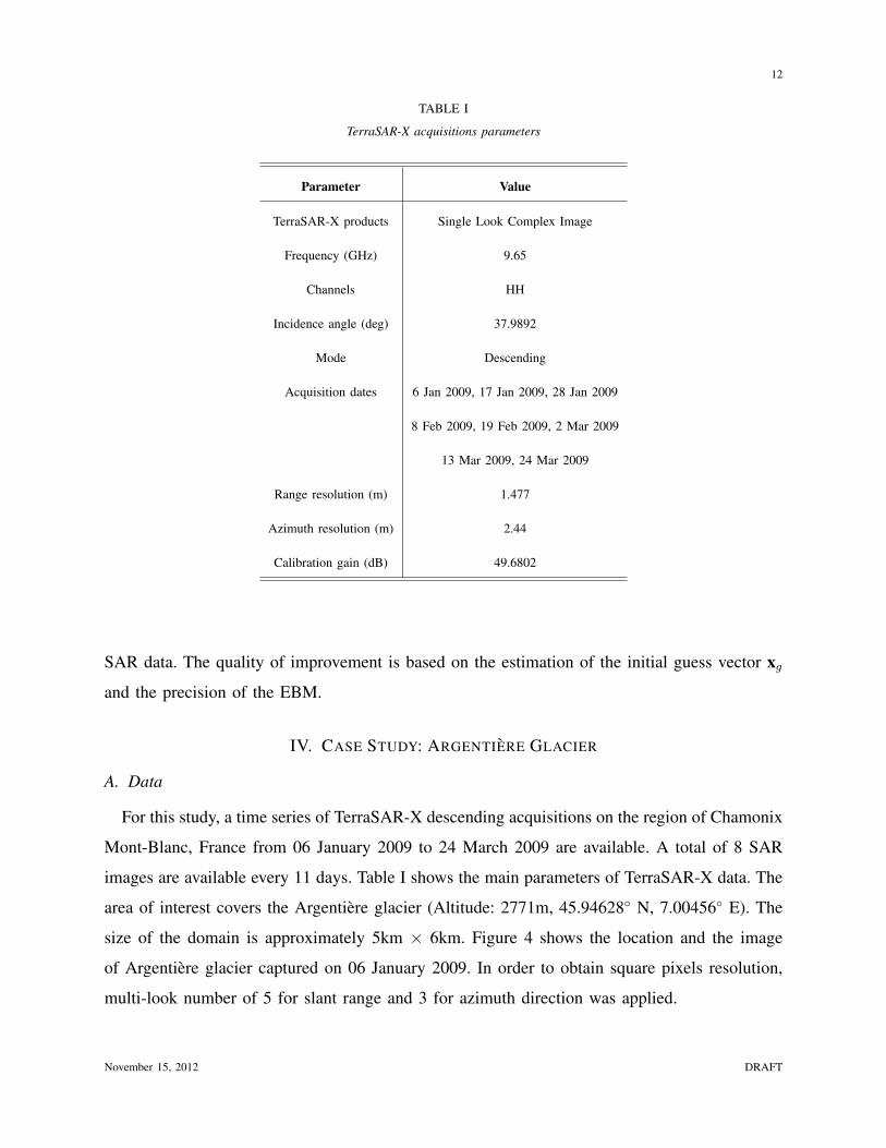
TABLE I

TerraSAR-X acquisitions parameters

Parameter Value

TerraSAR-X products Single Look Complex Image

Frequency (GHz) 9.65

Channels HH

Incidence angle (deg) 37.9892

Mode Descending

Acquisition dates 6 Jan 2009, 17 Jan 2009, 28 Jan 2009

8 Feb 2009, 19 Feb 2009, 2 Mar 2009

13 Mar 2009, 24 Mar 2009

Range resolution (m) 1.477

Azimuth resolution (m) 2.44

Calibration gain (dB) 49.6802

SAR data. The quality of improvement is based on the estimation of the initial guess vector xgand the precision of the EBM.

IV. CASE STUDY: ARGENTIERE GLACIER

A. Data

For this study, a time series of TerraSAR-X descending acquisitions on the region of Chamonix

Mont-Blanc, France from 06 January 2009 to 24 March 2009 are available. A total of 8 SAR

images are available every 11 days. Table I shows the main parameters of TerraSAR-X data. The

area of interest covers the Argentiere glacier (Altitude: 2771m, 45.94628◦ N, 7.00456◦ E). The

size of the domain is approximately 5km × 6km. Figure 4 shows the location and the image

of Argentiere glacier captured on 06 January 2009. In order to obtain square pixels resolution,

multi-look number of 5 for slant range and 3 for azimuth direction was applied.


13

��

��

��

Fig. 4. (Top) Location of the TerraSAR-X acquisition in the French Alps. (Bottom) The crop image on the Argentiere glacier

area. The snowpack stratigraphic profiles calculated by Crocus snow model are given for 3 different altitudes on the Argentiere

glacier: 2400m, 2700m and 3000m. The rectangles show the approximate positions of these altitudes on the TerraSAR-X images.

For this study, meteorological forcing data provided by SAFRAN at 2400, 2700, and 3000 m

altitude on horizontal terrain were used to drive the detailed snowpack model Crocus throughout

the whole season 2008-2009 (starting on August 1st 2008). In order to carry out the comparison

between the backscattering coefficients σsim (obtained from executing the EBM using Crocus

snowpack profile as input) and σTSX (obtained from TerraSAR-X reflectivity), they need to be

representative of the same area. Therefore we need to estimate the backscattering coefficients

that well-represent the SAR reflectivities of the studied areas. The characteristic of a snowcover

surface texture is spatially heterogeneous due to its strong variations of physical properties. A

Gaussian distributed SAR texture hypothesis is therefore invalid. In recent studies, it has been

proven that the texture of a SAR image of a heterogeneous medium can be modeled using the

Fisher probability distribution [21], [22]. From the parameters of Fisher probability distribution,

we can calculate the theoretical mean value which represents the backscattering coefficient of

an area. In this study, the representative values of the backscattering coefficients of SAR image

data on each altitude are obtained by calculating the mean value of Fisher-distributed texture of

three regions (Fig. 4) as in [22].


14

2 4 6 8 10 12 14−100

−80

−60

−40

−20

0

Frequency in Ghz

Back

scat

terin

g co

effic

ient

σvo

l0

in (d

B)

SurfaceGroundVolumeTotal

2 4 6 8 10 12 14−100

−80

−60

−40

−20

0

Frequency in Ghz

Back

scat

terin

g co

effic

ient

σvo

l0

in (d

B)

SurfaceGroundVolumeTotal

Fig. 5. Comparison of the contribution from surface, ground and volume backscattering mechanisms plotted in function of

frequency f . The roughness parameters of surface and ground are: Left: σh = 0.4cm and l = 8.4cm corresponding to slightly

rough and Right: σh = 1.12cm and l = 8.8cm corresponding to very rough (data taken from [23]). The volume backscattering

coefficient is simulated using the snow profile in Table II.

The roughness parameters of surface air-snow and ground are not available in the guess data

calculated by Crocus, therefore the empirical values of the correlation length and the rms height

have been taken from the measurements of Oh et. al. [23]. As we can see in figure 5, in the

high frequency range (more than 10GHz), the contribution of surface and ground contribution

are considerably low compared to the volume backscattering, regardless of slightly rough or

very rough surface. Therefore we only concentrate on the volume contribution on the tests of

data analysis method. According to the nature of a dry snow surface, the values of σh = 0.4cm

and l = 8.4cm with a Gaussian type of surface spectrum, which correspond to a slightly rough

surface, are used for the modeling in this study. With these surface and ground parameters set

to constants, the original input vector x = [xCrocus xs xg] in our case contains only the physical

parameters of each layer of snowpack, which has the following form:

x = [xCrocus] = [x1, x2, . . . , x2n]t = [d1, d2, . . . , dn, ρ1, ρ2, . . . , ρn]t (19)

where di and ρi are respectively the optical grain size and the density of ith layer of the snowpack.

On the first iteration of the algorithm, x = xg and xg is given by the Crocus snow profile.

The covariance matrix B, which represents the error of the input profile, i.e. of the Crocus


15

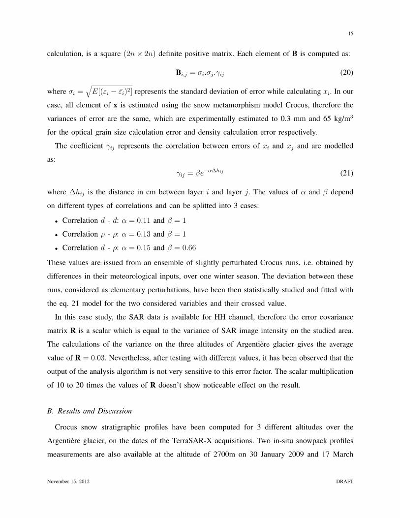
calculation, is a square (2n× 2n) definite positive matrix. Each element of B is computed as:

Bi,j = σi.σj.γij (20)

where σi =√E[(εi − εi)2] represents the standard deviation of error while calculating xi. In our

case, all element of x is estimated using the snow metamorphism model Crocus, therefore the

variances of error are the same, which are experimentally estimated to 0.3 mm and 65 kg/m3

for the optical grain size calculation error and density calculation error respectively.

The coefficient γij represents the correlation between errors of xi and xj and are modelled

as:

γij = βe−α∆hij (21)

where ∆hij is the distance in cm between layer i and layer j. The values of α and β depend

on different types of correlations and can be splitted into 3 cases:

• Correlation d - d: α = 0.11 and β = 1

• Correlation ρ - ρ: α = 0.13 and β = 1

• Correlation d - ρ: α = 0.15 and β = 0.66

These values are issued from an ensemble of slightly perturbated Crocus runs, i.e. obtained by

differences in their meteorological inputs, over one winter season. The deviation between these

runs, considered as elementary perturbations, have been then statistically studied and fitted with

the eq. 21 model for the two considered variables and their crossed value.

In this case study, the SAR data is available for HH channel, therefore the error covariance

matrix R is a scalar which is equal to the variance of SAR image intensity on the studied area.

The calculations of the variance on the three altitudes of Argentiere glacier gives the average

value of R = 0.03. Nevertheless, after testing with different values, it has been observed that the

output of the analysis algorithm is not very sensitive to this error factor. The scalar multiplication

of 10 to 20 times the values of R doesn’t show noticeable effect on the result.

B. Results and Discussion

Crocus snow stratigraphic profiles have been computed for 3 different altitudes over the

Argentiere glacier, on the dates of the TerraSAR-X acquisitions. Two in-situ snowpack profiles

measurements are also available at the altitude of 2700m on 30 January 2009 and 17 March


16

TABLE II

Snow stratigraphic profile obtained from an in-situ measurement on Argentiere glacier on 30 January 2009 at the altitude of

2700m.

Snow depth Thickness Grain size Density

(cm) (cm) (mm/10) (Kg/m3)

0

13 13 5 210

25 12 5 290

31 6 5 310

56 25 7.5 220

85 29 7.5 300

92 7 15 340

125 33 15 430

135 10 15 370

190 55 15 430

2009, and an example is shown in table II. The level of liquid water content per volume at

the time and location of measurement is below 2 percent, which means the snowpack can be

considered as dry snow. Fig. 4 shows the approximate locations of each study area on the glacier.

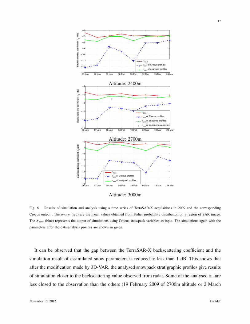
Fig. 6 shows the backscattering coefficients obtained over a period of time from three different

methods: TerraSAR-X reflectivities, Crocus simulated profiles and simulation of analyzed Crocus

profiles. Overall, the differences between the SAR reflectivities and the output of EBM simulation

using Crocus initial guess profiles are approximately 2 to 6 dB. The EBM can overestimate the

loss of EMW intensity while propagating through the snowpack medium due the assumption that

snow particles are of spherical shape. The definition of snow optical grain size, the calculation

of the effective permittivity and the phase matrix are also based on the same hypothesis. This

assumption does not always hold in the natural environment where snow particles can have

various shape and size. It is necessary to develop a more sophisticated method of modeling

interaction between EMW and snow particles of different geometry properties.


17

06 Jan 17 Jan 28 Jan 08 Feb 19 Feb 02 Mar 13 Mar 24 Mar−13

−12

−11

−10

−9

−8

−7

−6

Back

scat

terin

g co

effic

ient

σ0 (d

B)

σTSXσsim of Crocus profiles

σsim of analysed profiles

Altitude: 2400m


−12

−10

−8

−6

−4

Back

scat

terin

g co

effic

ient

σ0 (d

B)



σsim of in−situ measurement

Altitude: 2700m


−12

−11

−10

−9

−8

−7

−6

Back

scat

terin

g co

effic

ient

σ0 (d

B)



Altitude: 3000m

Fig. 6. Results of simulation and analysis using a time series of TerraSAR-X acquisitions in 2009 and the corresponding

Crocus output . The σTSX (red) are the mean values obtained from Fisher probability distribution on a region of SAR image.

The σsim (blue) represents the output of simulations using Crocus snowpack variables as input. The simulations again with the

parameters after the data analysis process are shown in green.

It can be observed that the gap between the TerraSAR-X backscattering coefficient and the

simulation result of assimilated snow parameters is reduced to less than 1 dB. This shows that

after the modification made by 3D-VAR, the analysed snowpack stratigraphic profiles give results

of simulation closer to the backscattering value observed from radar. Some of the analysed σ0 are

less closed to the observation than the others (19 February 2009 of 2700m altitude or 2 March


18

0 0.2 0.4 0.6 0.8 1 1.2 1.4

20406080

100120140160180200220

Snow grain size(mm)

Snow

dep

th(c

m)

Crocus ProfileAnalysed ProfileIn−situ measurements

0 100 200 300 400 500

20406080

100120140160180200220

Snow density(kg/m3)

Snow

dep

th(c

m)


−50 −45 −40 −35 −30 −25 −20 −15 −10 −5

20406080

100120140160180200220

Snow

dep

th(c

m)

σvol0 (dB)

Crocus profileAnalysed profileIn−situ measurements

Simulation from:

Date: 28 Jan 2009. Altitude: 2700m.

0 0.2 0.4 0.6 0.8 1 1.2 1.4

50

100

150

200

250

Snow grain size(mm)

Snow

dep

th(c

m)


0 100 200 300 400 500

50

100

150

200

250

Snow density(kg/m3)

Snow

dep

th(c

m)


−50 −45 −40 −35 −30 −25 −20 −15 −10 −5

50

100

150

200

250

Snow

dep

th(c

m)

σvol0 (dB)

Crocus profileAnalysed profileIn−situ measurements

Simulation from:

Date: 13 Mar 2009. Altitude: 2700m.

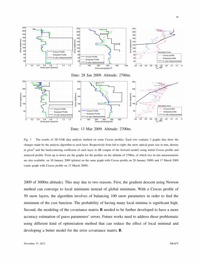
Fig. 7. The results of 3D-VAR data analysis method on some Crocus profiles. Each row contains 3 graphs that show the

changes made by the analysis algorithm to each layer. Respectively from left to right: the snow optical grain size in mm, density

in g/cm3 and the backscattering coefficient of each layer in dB (output of the forward model) using initial Crocus profile and

analyzed profile. From up to down are the graphs for the profiles on the altitude of 2700m, of which two in-situ measurements

are also available: on 30 January 2009 (plotted on the same graph with Crocus profile on 28 January 2009) and 17 March 2009

(same graph with Crocus profile on 13 March 2009).

2009 of 3000m altitude). This may due to two reasons. First, the gradient descent using Newton

method can converge to local minimum instead of global minimum. With a Crocus profile of

50 snow layers, the algorithm involves of balancing 100 snow parameters in order to find the

minimum of the cost function. The probability of having many local minima is significant high.

Second, the modeling of the covariance matrix B needed to be further developed to have a more

accuracy estimation of guess parameters’ errors. Future works need to address these problematic

using different kind of optimization method that can reduce the effect of local minimal and

developing a better model for the error covariance matrix B.


19

TABLE III

Comparison of bias and root-mean-square deviation (RMSD) between initial Crocus profiles and analysed profiles, with

respect to the in-situ measurements

Date Parameter Profile Bias RMSD

28 Jan 2009

Grain size (mm)Crocus 0.43 0.59

Analysed 0.45 0.57

Density (kg/m3)Crocus 110 120

Analysed 40 50

13 Mar 2009

Grain size (mm)Crocus 0.49 0.64

Analysed 0.46 0.61

Density (kg/m3)Crocus 120 130

Analysed 50 70

Fig. 7 shows the detailed of the modifications of snow stratigraphic profiles done by data

analysis process. The input parameters contain the snow optical grain size for Crocus, visually

estimated grain size for the in-situ measurements, and the density of each snow layer. It can be

observed that the modifications occur mostly on the near-surface layers. This can be due to two

reasons:

• The EMW at higher frequency has lower penetration rate. Depends on the compactness of

the snowpack environment, X-band EMW can penetrate from 80 to 120 cm. This means

the radar has little sensitivity to the characteristic of snowpack in the deeper layers. The

EBM has taken into account this penetration rate through the calculation of attenuation.

The deeper EMW penetrate, the higher value of attenuation is accumulated, and therefore

the backscattering coefficient of the snow layers decreases exponentially from the surface

layer to the ground layer. This can be observed from the graphs on third column of Fig. 7.

• The error covariance matrix of measurements B is calculated based on the error correlation

among layers. This correlation is based strongly on the distance between the layers (21).

Large distance between two layers results in low value of correlation. Therefore the modifi-

cations of the snow parameters of the near surface layers are considered independent from

the deeper layers.

Two in-situ measurements were carried out on 30 January 2009 (Tab. II) and 17 March 2009.


20

The stratigraphic profiles are plotted on the same graphs as the Crocus profiles of 28 January 2009

and 13 March 2009 (Fig. 7). The total simulated backscattering coefficients of these profiles are

also displayed on Fig. 6. We calculate the bias and root-mean-square deviation (RMSD) between

the initial (open-loop) Crocus profiles and the in-situ measurements, and compare to the bias and

RMSD between the analysed profiles and in-situ measurements. Table III shows the comparison

of these quantities. The results show the bias and RMSD between the analysed snow density

and the measurements are much smaller than the initial guess (Crocus) snow density, hence the

modifications made by the data analysis tend to approach the in-situ measurement. The analysis

however shows little improvement with the modifications on the snow optical grain size, due to

two reasons. First, the weight of the snow optical grain size in the covariance error matrix B,

as well as in the adjoint model, is bigger than the weight of snow density. Hence it can also

be noted that the values of optical grain size are not modified as much as the density (Fig. 7).

Second, the grain size used in Crocus is the snow optical radius, where the in-situ measurement

uses the visually estimated grain size. Therefore the two quantities are not directly comparable

to each other.

V. CONCLUSION

The results of this study show the potential of using data analysis method and the multilayer

snowpack backscattering model based on the radiative transfer theory in order to improve the

snowpack detailed simulation. The new backscattering model adapted to X-band and higher

frequencies enables the calculation of EMW losses in each layer of the snowpack more accurately.

Through the use of 3D-VAR data analysis based on the linear tangent and adjoint operator of the

forward model, we have the possibility to modify and improve the snowpack profiles calculated

by the detailed snowpack model Crocus. The output of this process shows that the discrepancies

between the simulated profile and the in situ measurements are smaller after assimilation, and

therefore could be further developed and used in real application such as snow cover area

monitoring on massif scale or snowpack evolution through a period of time using series of

spaceborne SAR image data.

Future studies will be concentrated on developing the assimilation process. The 3D-VAR

algorithm needs to be intergrated into Crocus, which means the analysed parameters of each

step will be used as the input for the next step of initialization of Crocus. The result will be


21

an intermittent assimilation process where the snow stratigraphic profile generated by Crocus is

continuously analysed and adjusted using TerraSAR-X data.

ACKNOWLEDGMENT

This work has been funded by GlaRiskAlp, a French-Italian project (2010-2013) on glacial

hazards in the Western Alps and Meteo-France. TerraSAR-X data was provided by German

Aerospace Center (DLR). In-situ measurements were carried out by IETR (University of Rennes

1), Gipsa-lab (Grenoble INP) and CNRM-GAME/CEN. The authors would like to thank Gilbert

Guyomarc’h, Matthieu Lafaysse and Samuel Morin from CNRM-GAME/CEN in carrying out

field measurements and performing the Crocus runs.

REFERENCES

[1] J. Shi and J. Dozier, “Estimation of snow water equivalence using sir-c/x-sar. i. inferring snow density and subsurface

properties,” Geoscience and Remote Sensing, IEEE Transactions on, vol. 38, no. 6, pp. 2465 – 2474, nov 2000.

[2] N. Longepe, S. Allain, L. Ferro-Famil, E. Pottier, and Y. Durand, “Snowpack characterization in mountainous regions

using c-band sar data and a meteorological model,” Geoscience and Remote Sensing, IEEE Transactions on, vol. 47, no. 2,

pp. 406 –418, feb. 2009.

[3] J. Koskinen, J. Pulliainen, K. Luojus, and M. Takala, “Monitoring of snow-cover properties during the spring melting

period in forested areas,” Geoscience and Remote Sensing, IEEE Transactions on, vol. 48, no. 1, pp. 50 –58, jan. 2010.

[4] F. T. Ulaby, R. K. Moore, and A. K. Fung, Microwave remote sensing: Active and passive. Volume III - From Theory to

Applications. Addison-Wesley, 1981.

[5] H. Wang, J. Pulliainen, and M. Hallikainen, “Extinction behavior of dry snow at microwave range up to 90 ghz by using

strong fluctuation theory,” Progress In Electromagnetics Research, vol. 25, pp. 39–51, 2000.

[6] A. Stogryn, “The bilocal approximation for the effective dielectric constant of an isotropic random medium,” Antennas

and Propagation, IEEE Transactions on, vol. 32, no. 5, pp. 517 – 520, may 1984.

[7] A. Fung, Z. Li, and K. Chen, “Backscattering from a randomly rough dielectric surface,” Geoscience and Remote Sensing,

IEEE Transactions on, vol. 30, no. 2, pp. 356 –369, mar 1992.

[8] A. Fung and K. Chen, “An update on the iem surface backscattering model,” Geoscience and Remote Sensing Letters,

IEEE, vol. 1, no. 2, pp. 75 – 77, april 2004.

[9] Y. Durand, E. Brun, L. Merindol, G. Guyomarc’h, B. Lesaffre, and E. Martin, “A meteorological estimation of relevant

parameters for snow models,” Journal of Glaciology, vol. 18, pp. 65–71, 1993.

[10] Y. Durand, G. Giraud, M. Laternser, P. Etchevers, L. Mrindol, and B. Lesaffre, “Reanalysis of 47 years of climate in

the French Alps (1958-2005): climatology and trends for snow cover,” Journal of Applied Meteorology and Climatology,

vol. 48, pp. 2487–2512, 2009.

[11] V. Vionnet, E. Brun, S. Morin, A. Boone, S. Faroux, P. Le Moigne, E. Martin, and J.-M. Willemet, “The detailed

snowpack scheme crocus and its implementation in surfex v7.2,” Geoscientific Model Development, vol. 5, no. 3, pp.

773–791, 2012. [Online]. Available: http://www.geosci-model-dev.net/5/773/2012/


http://www.geosci-model-dev.net/5/773/2012/

22

[12] P. Courtier, E. Andersson, W. Heckley, D. Vasiljevic, M. Hamrud, A. Hollingsworth, F. Rabier, M. Fisher, and J. Pailleux,

“The ECMWF implementation of three-dimensional variational assimilation (3D-Var). I: Formulation,” Quarterly Journal

of the Royal Meteorological Society, vol. 124, no. 550, pp. 1783 –1807, jan 1998.

[13] J. S. Lee and E. Pottier, Polarimetric Radar Imaging: From Basics to Applications. CRC Press, 2009.

[14] A. Martini, L. Ferro-Famil, and E. Pottier, “Polarimetric study of scattering from dry snow cover in alpine areas,” in

Geoscience and Remote Sensing Symposium, 2003. IGARSS ’03. Proceedings. 2003 IEEE International, vol. 2, july 2003,

pp. 854 – 856 vol.2.

[15] D. Floricioiu and H. Rott, “Seasonal and short-term variability of multifrequency, polarimetric radar backscatter of alpine

terrain from sir-c/x-sar and airsar data,” Geoscience and Remote Sensing, IEEE Transactions on, vol. 39, no. 12, pp. 2634

–2648, dec 2001.

[16] M. Hallikainen, F. Ulaby, and M. Abdelrazik, “Dielectric properties of snow in the 3 to 37 ghz range,” Antennas and

Propagation, IEEE Transactions on, vol. 34, no. 11, pp. 1329 – 1340, nov 1986.

[17] W. Huining, J. Pulliainen, and M. Hallikainen, “Effective permittivity of dry snow in the 18 to 90 ghz range,” Progress

In Electromagnetics Research, vol. 24, pp. 119 –138, 1999.

[18] N. Longepe, “Apport de l’imagerie sar satellitaire en bandes l et c pour la caracterisation du couvert neigeux,” Ph.D.

dissertation, Universite de Rennes 1, 2008.

[19] L. Tsang, J. Pan, D. Liang, Z. Li, D. Cline, and Y. Tan, “Modeling active microwave remote sensing of snow using dense

media radiative transfer (dmrt) theory with multiple-scattering effects,” Geoscience and Remote Sensing, IEEE Transactions

on, vol. 45, no. 4, pp. 990 –1004, april 2007.

[20] M. Dumont, Y. Durand, Y. Arnaud, and D. Six, “Variational assimilation of albedo in a snowpack model and reconstruction

of the spatial mass-balance distribution of an alpine glacier,” Journal of Glaciology, vol. 58(207), pp. 151–164, 2012.

[21] L. Bombrun and J.-M. Beaulieu, “Fisher distribution for texture modeling of polarimetric sar data,” Geoscience and Remote

Sensing Letters, IEEE, vol. 5, no. 3, pp. 512 –516, july 2008.

[22] O. Harant, L. Bombrun, G. Vasile, L. Ferro-Famil, and M. Gay, “Displacement estimation by maximum-likelihood texture

tracking,” Selected Topics in Signal Processing, IEEE Journal of, vol. 5, no. 3, pp. 398 –407, june 2011.

[23] Y. Oh, K. Sarabandi, and F. Ulaby, “An empirical model and an inversion technique for radar scattering from bare soil

surfaces,” Geoscience and Remote Sensing, IEEE Transactions on, vol. 30, no. 2, pp. 370 –381, mar 1992.


1 analysis of snowpack properties and structure from ... · recently launched high precision...

Documents