1

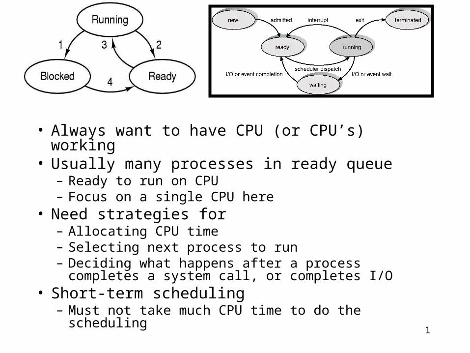
• Always want to have CPU (or CPU’s) working• Usually many processes in ready queue

– Ready to run on CPU– Focus on a single CPU here

• Need strategies for– Allocating CPU time– Selecting next process to run– Deciding what happens after a process completes a

system call, or completes I/O• Short-term scheduling

– Must not take much CPU time to do the scheduling

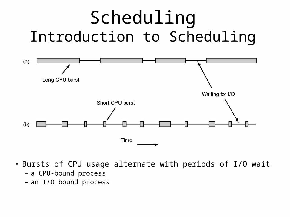
SchedulingIntroduction to Scheduling

• Bursts of CPU usage alternate with periods of I/O wait– a CPU-bound process– an I/O bound process

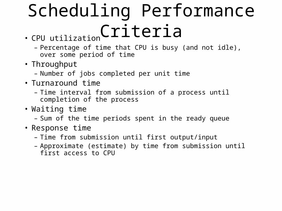
Scheduling Performance Criteria• CPU utilization

– Percentage of time that CPU is busy (and not idle), over some period of time

• Throughput– Number of jobs completed per unit time

• Turnaround time– Time interval from submission of a process until completion of the

process

• Waiting time– Sum of the time periods spent in the ready queue

• Response time– Time from submission until first output/input– Approximate (estimate) by time from submission until first access to CPU

4

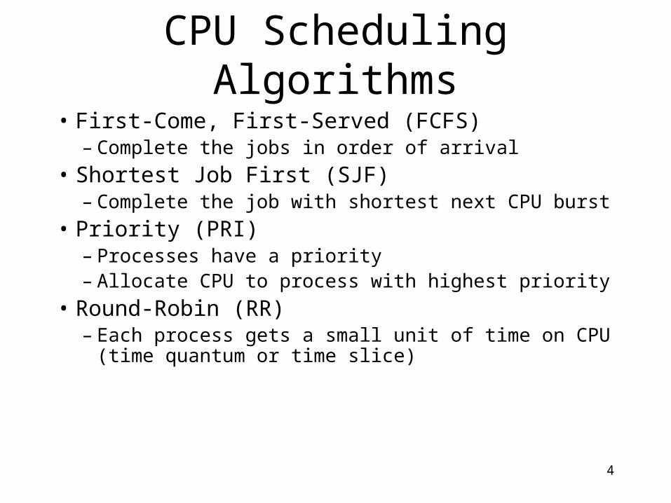
CPU Scheduling Algorithms

• First-Come, First-Served (FCFS)– Complete the jobs in order of arrival

• Shortest Job First (SJF)– Complete the job with shortest next CPU burst

• Priority (PRI)– Processes have a priority– Allocate CPU to process with highest priority

• Round-Robin (RR)– Each process gets a small unit of time on CPU (time

quantum or time slice)

5

Solution: Gantt Chart Method

• Waiting times?P1: 0P2: 20P3: 32P4: 40P5: 56

• Average wait time: 148/5 = 29.6

FCFS: First-Come First-Served

P1

20

P2

32

P3 P4 P5

40 56 600

6

FCFS: First-Come First-Served

• Advantage: Relatively simple algorithm

• Disadvantage: long waiting times

7

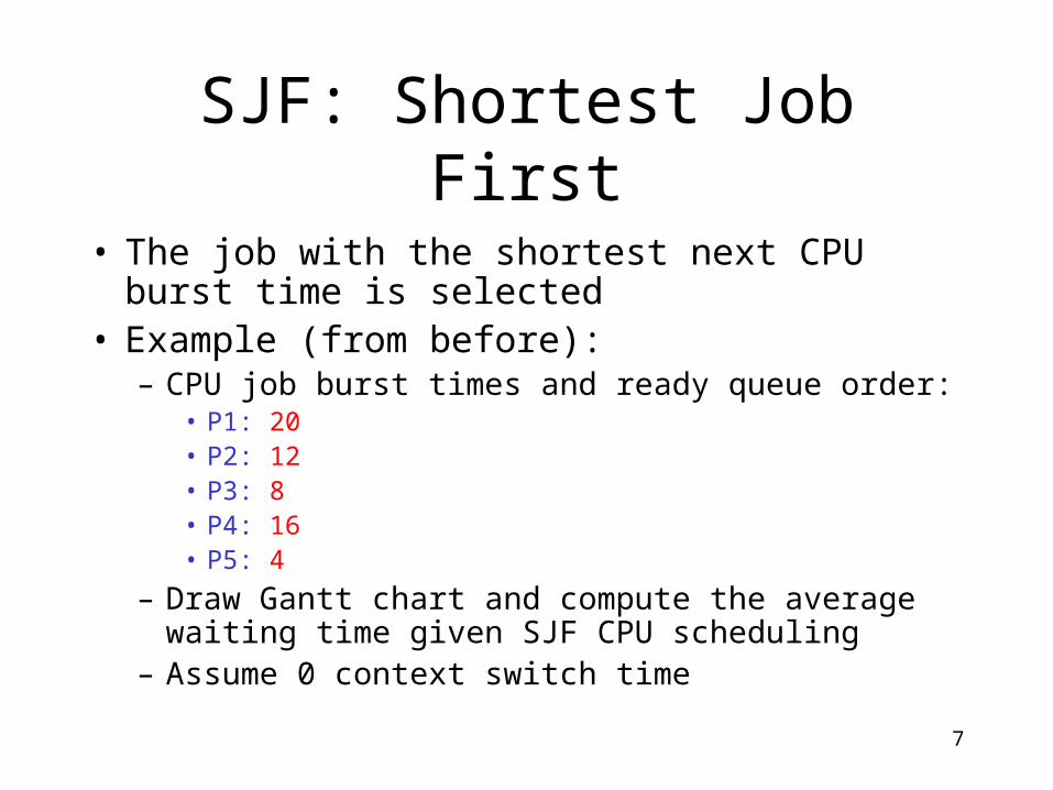
SJF: Shortest Job First

• The job with the shortest next CPU burst time is selected

• Example (from before):– CPU job burst times and ready queue order:

• P1: 20• P2: 12• P3: 8• P4: 16• P5: 4

– Draw Gantt chart and compute the average waiting time given SJF CPU scheduling

– Assume 0 context switch time

SJF Solution

• Waiting times (how long did process wait before being scheduled on the CPU?):P1: 40P2: 12P3: 4P4: 24P5: 0

• Average wait time: 16

(Recall: FCFS scheduling had average wait time of 29.6)

P1

4

P2

12

P3 P4P5

24 40 600

9

SJF

• Provably shortest average wait time

• BUT: What do we need to actually implement this?

10

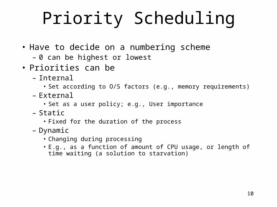
Priority Scheduling

• Have to decide on a numbering scheme– 0 can be highest or lowest

• Priorities can be– Internal

• Set according to O/S factors (e.g., memory requirements)

– External• Set as a user policy; e.g., User importance

– Static• Fixed for the duration of the process

– Dynamic• Changing during processing• E.g., as a function of amount of CPU usage, or length of time waiting (a

solution to starvation)

11

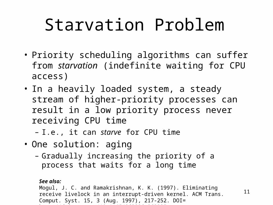
Starvation Problem

• Priority scheduling algorithms can suffer from starvation (indefinite waiting for CPU access)

• In a heavily loaded system, a steady stream of higher-priority processes can result in a low priority process never receiving CPU time– I.e., it can starve for CPU time

• One solution: aging– Gradually increasing the priority of a process that waits

for a long time

See also: Mogul, J. C. and Ramakrishnan, K. K. (1997). Eliminating receive livelock in an interrupt-driven kernel. ACM Trans. Comput. Syst. 15, 3 (Aug. 1997), 217-252. DOI= http://doi.acm.org/10.1145/263326.263335

12

Which Scheduling Algorithms Can be Preemptive?

• FCFS (First-come, First-Served)– Non-preemptive

• SJF (Shortest Job First)– Can be either– Choice when a new (shorter) job arrives– Can preempt current job or not

• Priority– Can be either– Choice when a processes priority changes or when a

higher priority process arrives

RR (Round Robin) Scheduling• Now talking about time-sharing or multi-tasking system

– typical kind of scheduling algorithm in a contemporary general purpose operating system

• Method– Give each process a unit of time (time slice, quantum) of

execution on CPU– Then move to next process in ready queue– Continue until all processes completed

• Necessarily preemptive– Requires use of timer interrupt

• Time quantum typically between 10 and 100 milliseconds– Linux default appears to be 100ms

13

14

RR (Round Robin) Scheduling: Example

• CPU job burst times & order in queue– P1: 20– P2: 12– P3: 8– P4: 16– P5: 4

• Draw Gantt chart, and compute average wait time– Time quantum of 4– Like our previous examples, assume 0 context

switch time

15

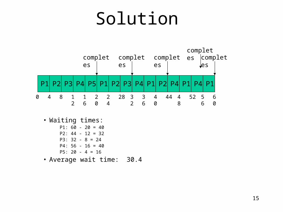
Solution

• Waiting times:P1: 60 - 20 = 40P2: 44 - 12 = 32P3: 32 - 8 = 24P4: 56 - 16 = 40P5: 20 - 4 = 16

• Average wait time: 30.4

P1 P2

4

P3 P4 P5 P1

8 12 16 20 24

P2 P3

28

P4 P1 P2 P4

32 36 40 44 48

P1 P4

52

P1

56 60

completes completes completes completescompletes

0

16

Other Performance Criteria

P1

20

P2

32

P3 P4 P5

40 56 60

FCFS

P1

4

P2

12

P3 P4P5

24 40 60

SJF

P1 P2

4

P3 P4 P5 P1

8 12 16 20 24

P2 P3

28

P4 P1 P2 P4

32 36 40 44 48

P1 P4

52

P1

56 60

RR

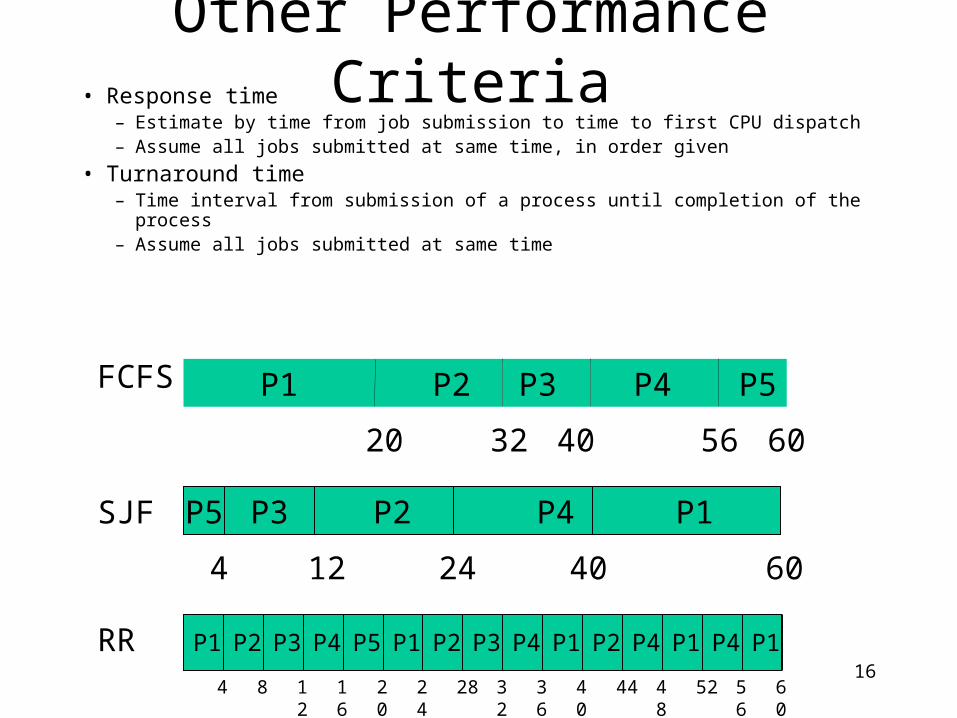
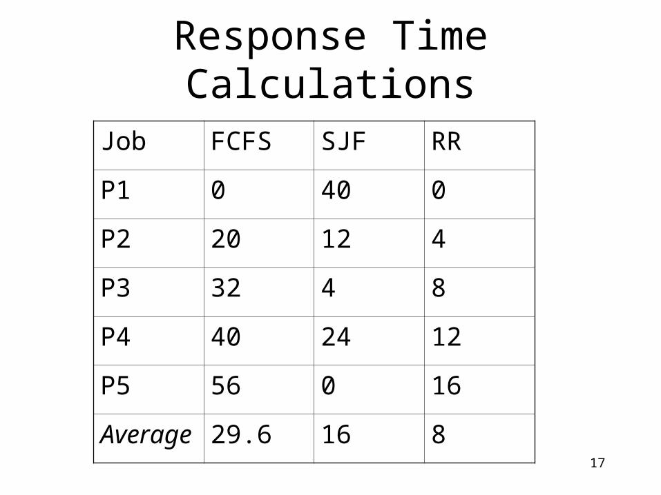
• Response time– Estimate by time from job submission to time to first CPU dispatch– Assume all jobs submitted at same time, in order given

• Turnaround time– Time interval from submission of a process until completion of the process– Assume all jobs submitted at same time

17

Response Time Calculations

Job FCFS SJF RR

P1 0 40 0

P2 20 12 4

P3 32 4 8

P4 40 24 12

P5 56 0 16

Average 29.6 16 8

18

Turnaround Time CalculationsJob FCFS SJF RR

P1 20 60 60

P2 32 24 44

P3 40 12 32

P4 56 40 56

P5 60 4 20

Average 41.6 28 42.4

19

Performance Characteristics of Scheduling Algorithms

• Different scheduling algorithms will have different performance characteristics

• RR (Round Robin)– Average waiting time often high– Good average response time

• Important for interactive or timesharing systems

• SJF– Best average waiting time– Some overhead with respect to estimates of CPU burst

length & ordering ready ‘queue’

20

Context Switching Issues

• This analysis has not taken context switch duration into account– In general, the context switch will take time– Just like the CPU burst of a process takes time– Response time, wait time etc. will be affected by

context switch time

• RR (Round Robin) & quantum duration– To reduce response times, want smaller time quantum

• But, smaller time quantum increases system overhead

21

Example

Calculate average waiting time for RR (round robin) scheduling, for Processes:

P1: 24 P2: 4 P3: 4

Assume above order in ready queue; P1 at head of ready queue

Quantum = 4; context switch time = 1

22

Solution: Average Wait Time With Context Switch Time

• P1: 0 + 11 + 4 = 15• P2: 5• P3:10• Average: 10

(This is also a reason to dynamically vary the time quantum. E.g., Linux 2.5 scheduler, and Mach O/S.)

P1 P2 P3 P1 P1 P1 P1 P1

4 5 9 10 14 15 19 20 24 25 29 30 34 35 39

23

Multi-level Ready Queues

• Multiple ready queues– For different types of processes (e.g., system, user)– For different priority processes (e.g., Mach)

• Each queue can– Have a different scheduling algorithm– Receive a different amount of CPU time– Have movement of processes to another queue (feedback)

• e.g., if a process uses too much CPU time, put in a lower priority queue

• If a process is getting too little CPU time, put it in a higher priority queue

24

Multilevel Queue Scheduling

25

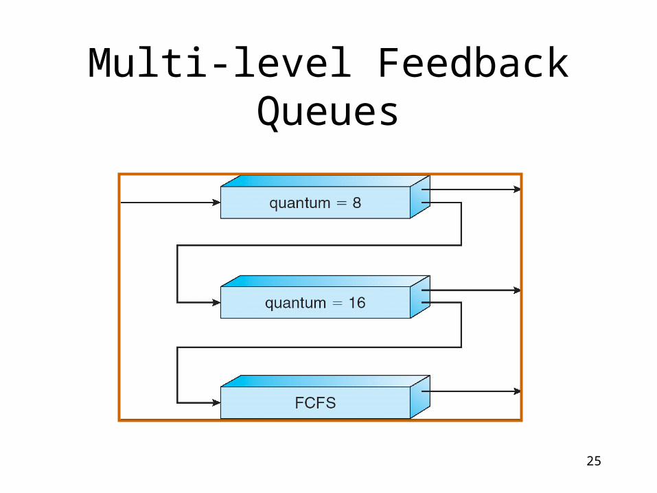
Multi-level Feedback Queues

Scheduling in Existing Systems: Linux 2.5 kernel

• Priority-based, preemptive

• Two priority ranges (real time and nice)

• Time quantum longer for higher priority processes (ranges from 10ms to 200ms)

• Tasks are runnable while they have time remaining in their time quantum; once exhausted, must wait until others have exhausted their time quantum

O(1) Background Briefly – the scheduler maintained two runqueues

for each CPU, with a priority linked list for each priority level (140 total).

Tasks are enqueued into the corresponding priority list.

The scheduler only needs to look at the highest priority list to schedule the next task.

Assigns timeslices for each task. Had to track sleep times, process interactivity, etc.

O(1) Background

Two runqueues per CPU, I said...one active, one expired. If a process hasn't used its entire timeslice, it's on the active queue; if it has, it's expired. Tasks are swapped between the two as needed.

Timeslice and priority are recalculated when a task is swapped.

If the active queue is empty, they swap pointers, so the empty one is now the expired queue.

O(1) Background

The first 100 priority lists are for real-time tasks, the last 40 are for user tasks.

User tasks can have their priorities dynamically adjusted, based on their dependency. (I/O or CPU)

CPU Scheduling as of Linux 2.6.23 Kernel: “Completely Fair Scheduler”

• Goal: fairness in dividing processor time to tasks• Balanced (red-black) tree to implement a ready queue;

O(log n) insert or delete time• Queue ordered in terms of “virtual run time”

– smallest value picked for using CPU

– small values: tasks have received less time on CPU

– tasks blocked on I/O have smaller values

– execution time on CPU added to value

– priorities cause different decays of values

30http://www.ibm.com/developerworks/linux/library/l-completely-fair-scheduler/

The Completely Fair Scheduler

CFS cuts out a lot of the things previous versions tracked – no timeslices, no sleep time tracking, no process type identification...

Instead, CFS tries to model an “ideal, precise multitasking CPU” – one that could run multiple processes simultaneously, giving each equal processing power.

Obviously, this is purely theoretical, so how can we model it?

CFS, continued We may not be able to have one CPU run things

simultaneously, but we can measure how much runtime each task has had and try and ensure that everyone gets their fair share of time.

This is held in the vruntime variable for each task, and is recorded at the nanosecond level. A lower vruntime indicates that the task has had less time to compute, and therefore has more need of the processor.

Furthermore, instead of a queue, CFS uses a Red-Black tree to store, sort, and schedule tasks.

Priorities and more While CFS does not directly use priorities or priority

queues, it does use them to modulate vruntime buildup.

In this version, priority is inverse to its effect – a higher priority task will accumulate vruntime more slowly, since it needs more CPU time.

Likewise, a low-priority task will have its vruntime increase more quickly, causing it to be preempted earlier.

“Nice” value – lower value means higher priority. Relative priority, not absolute...

RB Trees A red-black tree is a binary search tree, which means

that for each node, the left subtree only contains keys less than the node's key, and the right subtree contains keys greater than or equal to it.

A red-black tree has further restrictions which guarantee that the longest root-leaf path is at most twice as long as the shortest root-leaf path. This bound on the height makes RB Trees more efficient than normal BSTs.

Operations are in O(log n) time.

The CFS Tree

The key for each node is the vruntime of the corresponding task.

To pick the next task to run, simply take the leftmost node.

http://www.ibm.com/developerworks/linux/library/l-completely-fair-scheduler/

Modular scheduling Alongside the initial CFS release came the notion of

“modular scheduling”, and scheduling classes. This allows various scheduling policies to be implemented, independent of the generic scheduler.

sched.c, which we have seen, contains that generic code. When schedule() is called, it will call pick_next_task(), which will look at the task's class and call the class-appropriate method.

Let's look at the sched_class struct...(sched.h L976)

Scheduling classes!

Two scheduling classes are currently implemented: sched_fair, and sched_rt.

sched_fair is CFS, which I've been talking about this whole time.

sched_rt handles real-time processes, and does not use CFS – it's basically the same as the previous scheduler.

CFS is mainly used for non-real-time tasks.

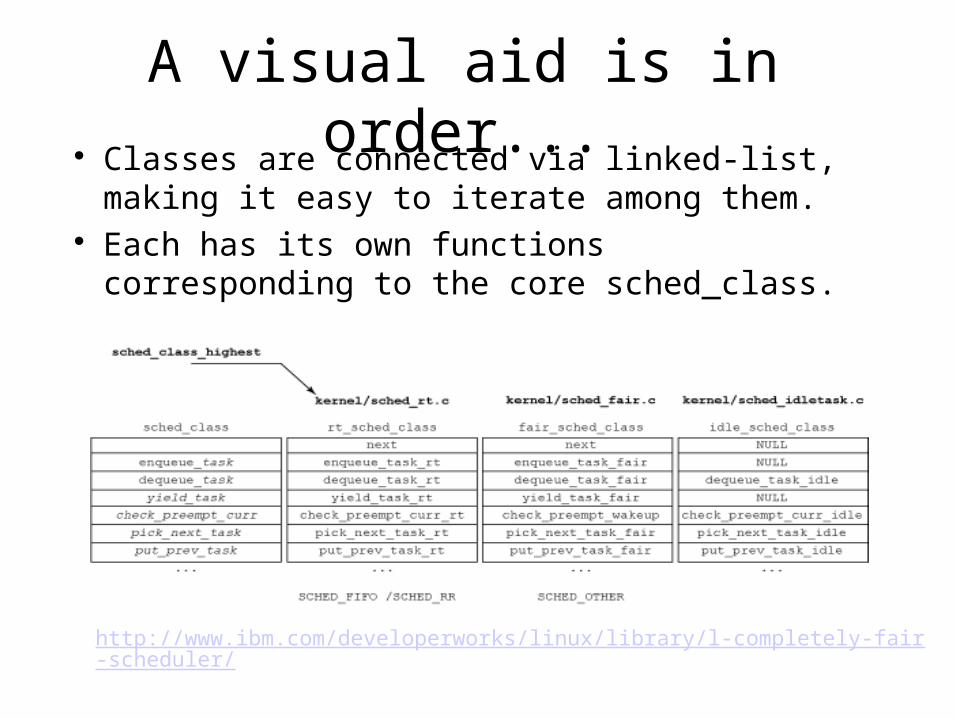
A visual aid is in order... Classes are connected via linked-list, making it easy to

iterate among them. Each has its own functions corresponding to the core

sched_class.

http://www.ibm.com/developerworks/linux/library/l-completely-fair-scheduler/