1

Absolute Calibration of Dual Frequency TimingReceivers for Galileo

B. P. B. Elwischger, S. Thoelert, M. Suess, J. FurthnerInstitute for Communications and Navigation, German Aerospace Center (DLR)

Muenchner Strasse 20, 82234 Oberpfaffenhofen, Germanymail: bernhard.elwischger@dlr.de

Abstract—The timing service of Global Navigation Satel-lite Systems (GNSS) is being steadily improved. Generally,this fact traces back to increasing accuracy of the providedephemeris data, improvements in Precise Point Positioning,continuous refinement of time transfer techniques, theutilization of modern signals, the use of wider bandwidth,and a growing number of available satellites—the latterparticularly due to the coexistence of an increasing numberof independent GNSSs available. The accuracy achievableby the GNSS common view time transfer method is withinrange of nanoseconds. In particular the upcoming Galileoin combination with the Global Positioning System isexpected to improve that accuracy even further.In this paper, we present results for an approach for abso-lute calibration of Galileo timing receivers operating in theL1BC and E5 signal bands. The internal receiver delays forGalileo E1 and GPS L1 signals of the institute’s SeptentrioPolaRx4 TR PRO are assessed. The approach utilizes ahardware simulator, which is an expanded version of aGSS7790 GNSS simulator from Spirent Communications.The simulator, the receiver under test, as well as the utilizedmeasurement equipment use the 10 MHz signal from thesame cesium clock as reference.

Keywords—Receiver calibration, multi frequency, GNSS,synchronization, time transfer

I. INTRODUCTION

With two-way satellite time and frequency transfer (TW-STFT) [7] “potentially even sub-nanosecond uncertaintycan be achieved” [5]. Multi-GNSS time and frequencytransfer will further push the limits. In this context, theneed for accurate calibration of the utilized equipment atnanosecond level draws more and more attention.GNSS time transfer requires calibration of the entiresynchronization chain of the station setup including an-tenna (i.e., its group delay, the coordinates of its phasecenter, aperture, etc.), cables, passive splitters, activesignal distributors, and the internal receiver delays ofthe GNSS timing receiver. Here, the calibration of theinternal receiver delays, which may differ by hundreds ofnanoseconds for different receiver models [12], is one ofthe most crucial issues.

We focus this paper on accurate calibration of multifrequency GNSS timing receivers for Galileo signals onnanosecond level. Results are given in comparison tocalibration results for GPS signals in the same setup.

A. Applications for satellite time and frequency transfer

It is a well-established approach to use the commonview technique for comparison of clocks located at differ-ent sites. It enables time scale generation in distributedsystems or networks, such as the International AtomicTime (TAI) [4]. TAI is generated by the InternationalBureau of Weights and Measure (BIPM) based on thecomparison of atomic frequency standards in variouslaboratories. A similar laboratory supporting TAI is locatedat our institute.Apart from that, satellite time and frequency transfer(STFT) can be utilized to provide syntonization or syn-chronization within any distributed system. If receptionof GNSS signals is available, such a system can spanthousands of kilometers. This enables e.g. maintenanceof consistency in globally distributed databases [3], ortime-based positioning using non-GPS signals [13].On the one hand, STFT can serve as a tool to monitorthe station clocks, in order to assess their stability. On theother hand, the time offsets determined by STFT can beused to correct the measured offsets between the stationclocks. Thus, synchronization errors are minimized, andprevented from masking other errors.

B. The need for absolute calibration

Absolute calibration is required for time transfer (i.e.,for synchronization of the stations’ clocks), but not for fre-quency transfer (i.e., syntonization of the stations’ clocks),which is illustrated in the following.

Assume a system of stations at different locations,including a clock each, and a single external clock. ForSTFT, that external clock would be a satellite clock. Eachstation can conduct time or frequency transfer of thatexternal clock through an individual time transfer chain. Ifthe system’s clocks are just to be synchronized to eachother but not to the external clock, then relative calibrationof the individual time transfer chains is sufficient. Thatcase merely enables frequency transfer of the individualclock to the network’s clocks (i.e., no time transfer).Synchronization of the system’s stations to the exter-nal clock, however, requires absolute calibration. It is aprerequisite for achieving time transfer from the externalclock to the individual stations’ clocks.

European Navigation Conference (ENC), Vienna 2013 ©by the authors

2

II. EXISTING METHODS FOR ABSOLUTE CALIBRATION

To calibrate a GNSS timing receiver there exist twocommon methods. One of those uses a fully calibratedreceiver often referred to as golden receiver (GR) to de-termine the internal delays of the device under test (DUT)based on the comparison between the GR and DUT. Thesecond method is based on hardware (HW) simulation ofthe GNSS signals, and came up with the development ofGNSS HW signal simulators. The following two sectionsgive a short description of these two established methods.

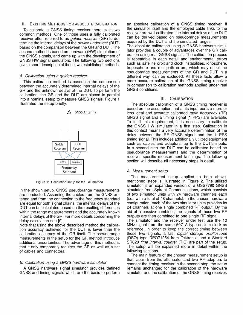
A. Calibration using a golden receiverThis calibration method is based on the comparison

between the accurately determined internal delays of theGR and the unknown delays of the DUT. To perform thecalibration, the GR and the DUT are placed in parallelinto a nominal setup to measure GNSS signals. Figure 1illustrates the setup briefly.

Golden Receiver

DUT Receiver

Frequency Standard

GNSS Antenna

1 PPS 10 MHz

Figure 1: Calibration setup for the GR method

In the shown setup, GNSS pseudorange measurementsare conducted. Assuming the cables from the GNSS an-tenna and from the connection to the frequency standardare equal for both signal chains, the internal delays of theDUT can be calculated based on the resulting differenceswithin the range measurements and the accurately knowninternal delays of the GR. For more details concerning thedelay calculation see [9].Note that using the above described method the calibra-tion accuracy achieved for the DUT is lower than thecalibration accuracy of the GR itself. The pseudorangemeasurements in the setup for the GR method introduceadditional uncertainties. The advantage of this method isthat it only temporarily requires the GR as well as a setof cables and connectors.

B. Calibration using a GNSS hardware simulatorA GNSS hardware signal simulator provides defined

GNSS and timing signals which are the basis to perform

an absolute calibration of a GNSS timing receiver. Ifthe simulator itself and the employed cable links to thereceiver are well calibrated, the internal delays of the DUTcan be derived based on pseudorange measurementsacquired by the DUT and the simulated ranges.The absolute calibration using a GNSS hardware simu-lator provides a couple of advantages over the GR cali-bration using real GNSS signals. The calibration processis repeatable in each detail and environmental errorssuch as satellite orbit and clock instabilities, ionosphere,troposphere and multipath errors, which may effect thepseudorange measurements of the GR and DUT in adifferent way, can be excluded. All these facts allow amore accurate calibration of the GNSS timing receiverin comparison to calibration methods applied under realGNSS conditions.

III. CALIBRATION

The absolute calibration of a GNSS timing receiver isbased on the assumption that at its input ports a more orless ideal and accurate calibrated radio frequency (RF)GNSS signal and a timing signal (1 PPS) are available.To fullfil this requirement, it is necessary to calibratethe GNSS HW simulator in a first step. Calibration inthis context means a very accurate determination of thedelay between the RF GNSS signal and the 1 PPStiming signal. This includes additionally utilized equipmentsuch as cables and adaptors, up to the DUT’s inputs.In a second step the DUT can be calibrated based onpseudorange measurements and the determination ofreceiver specific measurement latchings. The followingsection will describe all necessary steps in detail.

A. Measurement setupThe measurement setup applied to both above-

mentioned steps is illustrated in Figure 2. The utilizedsimulator is an expanded version of a GSS7790 GNSSsimulator from Spirent Communications, which consistsof two simulator units with 24 hardware channels each(i.e., with a total of 48 channels). In the chosen hardwareconfiguration, each of the two simulator units provides its24 channels at one single combined RF output. By theaid of a passive combiner, the signals of those two RFoutputs are then combined to one single RF signal.The simulator and the receiver under test use the 10MHz signal from the same 5071A type cesium clock asreference. In order to keep the correct timing betweenthose two signals, a fast digital storage oscilloscope(DSO) type DPO71254 from Tektronix, and a StanfordSR620 time interval counter (TIC) are part of the setup.The setup will be explained more in detail within thefollowing sections.

The main feature of the chosen measurement setup isthat, apart from the attenuator and two RF adapters toconnect the timing receiver in the second step, the setupremains unchanged for the calibration of the hardwaresimulator and the calibration of the GNSS timing receiver.

3

LNA(30 dB)

Time Interval Counter Atomic Clock

Reference Input

GNSS ReceiverTiming Output (1 PPS)

RF Input / Ch 1 Input

Timing Input (1 PPS) / Ch 2 Input

Reference InputTiming Inputs (1 PPS)

Monitor Output (RF)

Monitor Output (RF)

Reference Input

GNSS Simulator 2 (Slave)

Frequency Distributor

Attenuator(80 dB)

GNSS Simulator 1 (Master) Passive Combiner

Digital Storage Oscilloscope

orGNSS Receiver

1 PPSDistributor

Timing Output (1 PPS)

Figure 2: The hardware setup for simulator calibration is composed of all components marked in black and blue, for receiver calibration of allcomponents and connections marked in black and green.

B. Utilized satellite constellations & signalsConcerning the satellite constellations for calibration,

focus is given to geostationary (GEO) satellites.This avoids introduction of additional errors caused bynonperfect Doppler correction and consequent distortionsof the correlation function within the signal processing.

1) Constellations for simulator calibrationFor simulator calibration, the constellation can be de-

signed as simple as possible. Since the channels of thehardware simulator have to be calibrated individually, theycan be calibrated for satellites placed on the same posi-tion. This can be achieved either by using a constellationmerely consisting of one single satellite, which is thenswitched between the channels for individual simulatorchannel measurements. Or a constellation of 12 GEOsatellites at one position is used, so that only a singlechannel is set active for each individual simulator channelmeasurement. For this study, the latter approach is used.Separate recording of each satellite allows direct identifi-cation of the complex baseband signal, and simple carrierphase correction prior to individual correlation of its in-phase or quadrature component with the correspondingcode. Furthermore, this approach prevents the ocurrenceof eventual channel cross-correlations [8].

In the utilized configuration of the HW simulator forL1, L2, E1, and E5, the signals of 12 GPS and 12Galileo satellites could be simulated simultaneously.The 12 GEO satellites of one constellation can beequally distributed along a circle segment in the plane

x := 0 in Earth-centered, Earth-fixed (ECEF) Cartesiancoordinates.

2) Constellations for receiver calibration

The results presented in this paper are based on aGalileo constellation with 12 GEO satellites, a mixedGalileo constellation, and a mixed GPS constellation.Each of those two mixed constellations consists of 28medium earth orbit (MEO) satellites of the nominal con-stellation in addition to 4 GEO satellites. The GPS con-stellation is simulated simultaneously with either one ofthe two Galileo constellations. As the utilized hardwareconfiguration of the hardware simulator is limited to anumber of 12 instantaneous satellites per constellation,simulation is limited to an instantaneous number of 8MEO and 4 GEO satellites for the mixed constellations.Additional satellites in view are automatically droppedby the simulation software through geometric dilusion ofprecision (GDOP) selection.

On the one hand, GEO satellites may result in a lowervariance in the pseudorange measurements [14]. Further-more, simulation of satellites along curved paths by theHW simulator is non-ideal, as the simulator determinesthe ranges between the satellites and the user only fordiscrete points in time, and interpolates for the timeperiods in between.

On the other hand, the timing receiver requires anumber of at least 4 satellites in a geometry with sufficientGDOP for proper operation. For a pure GEO constella-tion, fulfillment of that requirement would be problematic.

4

3) Used signalsTable 1 shows the GNSS signals emitted by the HW

simulator in the utilized hardware configuration1. The lastcolumn lists the actual signal levels at the two combinedGNSS monitor outputs of the HW simulator. Initially, themeasurements and analysis are performed using theGalileo E1 signal, and for comparison the GPS L1 signalwas measured as well.

C. GNSS HW simulator calibrationThe calibration of the hardware simulator itself is

achieved by analysis of the simulated RF GNSS signalfrom a GPS or Galileo satellite constellation in relationto the 1 PPS signal the simulator generates from itsreference. Additionally all equipment up to the DUT’sphysical inputs is included within this analysis. Thatmeans that finally we determine the relation betweenRF and 1 PPS signal up to the DUT input connectorsas accurately as possible. For that purpose both signalsare captured in parallel with the DSO. Here, the 1 PPSsignal serves both as input and trigger signal.

1) Bias determinationPerforming the analysis of the delay between GNSS

signal and 1 PPS signal two approaches are suitable:— bias analysis by code correlation: After RF and 1

PPS signal have been captured using the oscilloscope,the RF signal is mixed down to baseband, and de-modulated. This demodulated baseband signal is thencorrelated with the expected GNSS code sequence todetermine the begin of a code epoch. The resultingdifference between the 1 PPS signal and the correlationpeak and consequently the begin of the code epochrepresents the simulator bias. During the calibration cam-paign it was found out that the simulator bias dependson the used hardware channel, and on the used signal(frequency and GNSS type). Figure 3 shows the resultsof the HW simulator calibration. The resulting hardwarechannel dependency is caused by the imperfect inter-channel calibration of the simulator. It is noted that thesimulator is within the specifications concerning the inter-channel bias, but to achieve an accuracy below 1 nsconcerning the receiver calibration we have to improvethe inter-channel bias calibration of the HW simulatorusing the explained calibration method.

— bias analysis by the dip in the amplitude: Asimple and practical approach that avoids the necessityof correlation processing, is the assessment of thesimulator bias by the dip in the amplitude. For absolutecalibration of GNSS timing receivers, it was first proposedin [15]. GNSS RF signals may have the characteristic thatduring the code transition the amplitude becomes zero.The difference between this so-called dip and the 1 PPSsignal represents also the simulator bias. Dependent on

1It is denoted as “12L1+12L2+12E1+12E5 Combined Output”.

the signal structure, this method may not be suitable forall signals of all existing GNSS systems. Besides, theapproach is not as accurate as code correlation.

2) Measurement requirementsTo achieve accurate results for the simulator bias, the

measurement setup requires reasonable settings.The record length for the DSO measurements dependson the used bias analysis method. Concerning themethod based on correlation, which is used in this work,two major aspects dictate the record length. One of theseconstraints is the underlying GNSS signal, in particular itscode length. Data acquisition of at least one code lengthis required, and averaging over several code lengths wasapplied to reduce measurement uncertainties.Furthermore, the record length seems to be a matter ofclock stability. Within the data record interval, the clockstability must remain within a certain bound to guaranteethat the error budget is met. For the cesium clock, thetime domain stability is provided as root Allan varianceσy(2, τ), i.e., as function of the averaging time τ . For anaveraging time of 10 ms, it stays below 75 ps, and for100 ms below 12 ps [1]. Hence, the maximum error dueto clock instability can be estimated as below 0.1 ns fora correlation data length greater or equal than 10 ms.

Recording the RF signals in the time domain withthe oscilloscope, the analogue bandwidth of the usedoscilloscope should be at least 1.6 GHz to maintain thefull bandwidth of the Galileo E1 and E5 RF signals inthe time domain, compare Table 1. The DSO used forthis study provides an analogue bandwidth of 12.5 GHz.The sampling rate is set to 25 GS/s to maintain the fullanalog bandwidth of the sampled signals according tothe Nyquist-Shannon theorem. That prevents aliasing incase residual noise from the hardware simulator at higherfrequencies is present. We additionally amplify with a low-noise amplifier (LNA) providing 30 dB amplification, inorder to reach voltage levels which the DSO can track.

As there is only one timing output of GNSS Simulator1 available, an active 1 PPS distribution amplifier is usedfor distribution either to DSO or GNSS receiver, in parallelto the TIC. An active distribution amplifier is preferred toa passive splitter in order to ensure defined and sufficientsignal levels. Furthermore, it eases connection of deviceswith different input impedances parallel to each other tothe timing output of the HW simulator.

D. Receiver calibrationWithin the timing receiver we have to consider two

aspects. These are the delay of the GNSS signal withinthe receiver hardware which is referred as "internaldelay", and the timing delay which is also referred as"measurement latching". For the used Septentrio receiverthe measurement latching can be determined using aTIC. The timing delay depends on the receiver model aswell as on the relation between the 10 MHz referencesignal and the 1 PPS signal. In a fixed setup the timing

5

Carrier [MHz] Signal Type Modulation Chipping rate Code length Full length [ms] power level

L1: 1575.42 C/A Data BPSK 1.023 Mcps 1023 1 -60 dBmP Precise BPSK 10.023 Mcps 7 days 7 days -63 dBm

L2: 1227.60 P Precise BPSK 10.023 Mcps 7 days 7 days -66 dBm

E1: 1575.42 B Data BOC(1,1) 1.023 Mcps 4092 ∗ 1 4 -58 dBmC Pilot BOC(1,1) 1.023 Mcps 4092 ∗ 25 100 -58 dBm

E5a: 1176.450 a-I Data AltBOC(15, 10) 10.23 Mcps 10230 ∗ 20 20 -58 dBma-Q Pilot AltBOC(15, 10) 10.23 Mcps 10230 ∗ 100 100 -58 dBm

E5b: 1207.140 b-I Data AltBOC(15, 10) 10.23 Mcps 10230 ∗ 4 4 -58 dBmb-Q Pilot AltBOC(15, 10) 10.23 Mcps 10230 ∗ 100 100 -58 dBm

Table 1: Galileo signals provided by the GNSS HW simulator, following [2].

delay is constant and unaffected by power cycles ofthe receiver. Given that timing delay, the internal delayof the receiver can be determined by comparison ofthe code range measurements of the simulated satelliteconstellation to the actual range between the individualsatellites and the simulated user position.

In order to extract the internal receiver delay from a re-ceiver’s pseudorange measurements, the correspondingequation for the internal receiver delay ∆tRx for a specificcode signal on a particular carrier has to be solved:

∆tRx =P −R

c0+ ∆trel − ∆ttrop − ∆tiono − ∆tRF

+∆tref + ∆tRxref − REFSV − biassim,(1)

where REFSV denotes the clock offset between thereference clock of the HW simulator and the satellitetime, P the pseudorange measurement, R the true range,c0 the speed of light in vacuum, ∆trel the relativisticcorrection [6], ∆ttrop the tropospheric correction, ∆tionothe ionospheric correction, ∆tRF the antenna cable delayfrom the antenna/simulator to the receiver, ∆tref thetiming reference cable delay, ∆tRxref the receiver internalclock delay (denoted by Septentrio as “latching delay”),and biassim the time span that the generated GNSSsignal lags behind the generated 1 PPS signal of the HWsimulator. The latter is sometimes referenced as “tick-to-code delay” [10]. Utilization of a HW simulator offers thepossibility for simple cancellation of unnecessary termsby disabling them within the simulator control software,e.g. neglect atmospheric effects and simulate satelliteclocks that strictly follow their time system (i.e., thesatellites’ clocks yield neither bias nor drift). Equation (1)becomes

∆tRx =P −R

v0− ∆tRF + ∆tref + ∆tRxref − biassim.

(2)

If we define

∆tDSO = ∆tRF − ∆tref + biassim, (3)

we obtain

∆tRx =P −R

v0− ∆tDSO + ∆tRxref . (4)

The aggregated time delay ∆tDSO is only valid for a spe-cific signal on a particular carrier, and to be determinedby the use of a DSO, see Figure 2. In addition to signaltype and carrier, this delay also varies between channelsof the HW simulator. Hence ∆tDSO should be determinedindividually for each channel if more than one channel ofthe HW simulator is required for calibration.

Note that concerning the receiver calibration, an atten-uator is interconnected in order to reduce the signal level(C/N0) so that it can be tracked by the receiver.

IV. RESULTS

In the first step, the simulator including all connectionsis calibrated. The calibration is referenced to the inputports of the receiver, and conducted for GPS L1 andGalileo E1 signals. After that, the internal delays of aPolaRx4 TR PRO for those signals are determined.The signal power levels of the satellites belonging to thesame constellation are set to the same constant valueprovided in Table 1 (i.e., rather than making them dependon the range between satellite and user).

A. Simulator calibration resultsAs mentioned before, the simulator has 48 channels.

The utilized hardware configuration provides Galileo E1and E5 signals, and GPS L1 and L2 signals, with 12channels for each signal. For this study, 24 channels areexamined, as we focus on comparisons between GPS L1and Galileo E1. The HW simulator calibration is basedon GEO satellites according to Section III-B1, with thesignals of only one single satellite active at a time. Thus,the HW simulator is calibrated channel per channel bythe correlation method described in Section III-C1.Figure 3 shows the resulting HW simulator inter-channelbias for GPS L1 C/A code and Galileo E1 data code,individually for each of the HW simulator’s channels. Thedata in Figure 3 are obtained from correlation with about30 code lengths for GPS L1 C/A code, and 10 codelengths for Galileo E1 data code. The number for thelatter was chosen lower, as it is four times the lengthof the former, see Table 1. The standard deviation isalso provided. The average bias has been subtracted tohighlight the inter-channel bias. A polynomial fit is applied

6

1 2 3 4 5 6 7 8 9 10 11 12−1

−0.5

0

0.5

1

1.5

GNSS HW simulator channel

Inte

rcha

nnel

bia

s an

d its

sta

ndar

d de

viat

ion

[ns]

GPS L1 C/A: meanGPS L1 C/A: sigmaGalileo E1 B (Data): meanGalileo E1 B (Data): sigma

Figure 3: HW simulator inter-channel biases & standard deviation

to the 1 PPS signal, reducing measurement noise andavoiding limitation of the measurement precision by thesampling interval of 40 ps.

B. Receiver calibration resultsThe internal receiver delay ∆tRx of the institute’s

Septentrio PolaRx4 TR PRO for Galileo E1 and GPS L1signals is assessed by measurement of pseudorangesfor a time span of about 8 hours, and application ofEquation (4). The applied GPS constellation (see SectionIII-B2) consists of the nominal constellation with a littlemodification: the satellites with pseudorandom noise(PRN) codes 29 to 32 are GEO. For the mixed Galileoconstellation, the MEO satellites with PRNs 1 to 28belong to the nominal constellation, with additional GEOsatellites. The second Galileo constellation consists of12 GEO satellites. The measurement interval is 1 second.

1) Internal delay for Galileo E1Figure 4 illustrates the receiver internal delay ∆tRx

for Galileo E1 over time, independently for each MEOsatellite of the mixed Galileo constellation. Based onaveraging the measurements shown in Figure 4, Figure5 provides the mean internal delay, and the standarddeviation σ, both individually for each satellite.

The results for the second Galileo constellation,which consists of 12 GEO satellites, are provided inFigure 6. Here, the assignment of the 12 simulated E1satellites’ signals to the HW simulator channels as wellas to the receiver channels is fixed throughout the entiremeasurement period2.

2The PRNs 1 to 12 were assigned to the 12 HW simulator channelsin consecutive order. The assigned GNSS timing receiver channelswere: 40, 44, 48, 28, 29, 30, 31, 32, 51, 52, 3, and 4.

4 5 6 7 8 10 11 12 13 14 18 19 20 24 25 26 2734.5

35

35.5

36

36.5

37

37.5

38

38.5

Galileo PRN

mea

n in

tern

al d

elay

and

sta

ndar

d de

viat

ion

[ns]

Figure 5: Internal delay and σ for Galileo E1 from MEO satellites.

01 02 03 04 05 06 07 08 09 10 11 1234.5

35

35.5

36

36.5

37

37.5

38

38.5

mea

n in

tern

al d

elay

and

sta

ndar

d de

viat

ion

[ns]

Galileo PRN

Figure 6: Internal delay and σ for Galileo E1 from GEO satellites.

2) Internal delay for GPS L1

The internal delay based on GPS C/A and P codemeasurements in the L1 band is determined in a similarmanner as for Galileo. Separately for each satellite, themean internal delay and the standard deviation fromthat mean internal delay is illustrated in Figure 7 for C/Acode, and in Figure 8 for P code. Both figures are basedon the simulator calibration for C/A code.The utilized GPS constellation is the mixed constellationdescribed in Section III-B2. The satellites with PRNs 1to 28 are MEO satellites, the ones with PRNs 29 to 32are GEO satellites. The figures suggest that varianceand bias are higher for the GEO satellites, in particularfor C/A code measurements.

7

0 0.5 1 1.5 2 2.5

x 104

35.8

36

36.2

36.4

36.6

36.8

37

time [s]

inte

rnal

del

ay [n

s]

E04E05E06E07E08E10E11E12E13E14E18E19E20E24E25E26E27

Figure 4: Internal delay of the PolaRx4 TR PRO for the Galileo E1 signal of the MEO satellites over time.

2 4 6 8 10 12 14 16 18 20 22 24 26 28 30 3234.5

35

35.5

36

36.5

37

37.5

38

38.5

GPS PRN

mea

n in

tern

al d

elay

and

sta

ndar

d de

viat

ion

[ns]

Figure 7: Internal delay and σ for GPS L1 C/A code signals from MEOsatellites (G01 to G28), and from GEO satellites (G29 to G32).

3) Dependency on the utilized receiver channel

A possible source of the differences of the internalreceiver delays for signals emitted by GEO satelliteswas suggested to be differences in the utilized receiverchannels. In another calibration measurement for GalileoE1 signals similar to the one presented in Figure 6, theassignment of the receiver channels was dynamicallychanged through the “RxControl” software that came withthe receiver. The plot of the internal receiver delay overtime in Figure 9 shows no noticeable change.It was verified that the receiver indeed switched theassigned channels. This was achieved by interpreting thedata stream from the receiver, which includes informationabout which measured signal is assigned to which chan-nel for every measurement epoch.

2 4 6 8 10 12 14 16 18 20 22 24 26 28 30 3234.5

35

35.5

36

36.5

37

37.5

38

38.5

GPS PRN

mea

n in

tern

al d

elay

and

sta

ndar

d de

viat

ion

[ns]

Figure 8: Internal delay and σ for GPS L1 P code signals from MEOsatellites (G01 to G28), and from GEO satellites (G29 to G32).

C. Final results

The resulting uncertainties including the total root sumof squares (RSS) are summarized in Table 2. As thequality of the results differed for GEO and MEO satellites,evaluation is done separately. The first row of Table 2shows the average standard deviation per channel forthe HW simulator calibration, obtained from the datapresented in Figure 3. It is 0.08 ns for Galileo E1 datacode, and 0.03 ns for GPS L1 C/A code.The numbers for the standard deviation of the meaninternal delays are provided in the second row. For GalileoE1, the standard deviation is gained from 17 single valuesfor MEO satellites (see Figure 5), and from 12 for GEOsatellites (see Figure 6). The numbers for GPS L1 arebased on 19 single values for MEO satellites, and on 4

8

Uncertainy E1 (GEO) E1 (MEO) L1 C/A (GEO) L1 C/A (MEO) L1 P (GEO) L1 P (MEO) IS bias affectedHW simulator 0.08 ns 0.08 ns 0.03 ns 0.03 ns ≈0.03 ns ≈0.03 ns yespseudoranges 0.7 ns 0.05 ns 0.58 ns 0.10 ns 0.13 ns 0.11 ns yesadapter 0.05 ns 0.05 ns 0.05 ns 0.05 ns 0.05 ns 0.05 ns no1 PPS edge 0.5 ns 0.5 ns 0.5 ns 0.5 ns 0.5 ns 0.5 ns in partsatomic clock 0.1 ns 0.1 ns 0.1 ns 0.1 ns 0.1 ns 0.1 ns noRSS 0.87 ns 0.52 ns 0.77 ns 0.52 ns 0.53 ns 0.52 ns

Table 2: Uncertainties for the measurement setup for the Septentrio PolaRx4 TR PRO GNSS timing receiver.

0 2000 4000 6000 8000 10000

35

36

37

38

internal receiver delay for individual satellite PRNs

time [s]

inte

rnal

del

ay [n

s]

0 2000 4000 6000 8000 100001

10

20

30

40

50

receiver channels used for tracking

time [s]

rece

iver

cha

nnel

no.

10000

E01E02E03E04E05E06E07E08E09E10E11E12

Figure 9: Internal delay over time for the signals of Galileo E11 andE12 switched between different receiver channels.

values for GEO satellites (see Figure 7 and Figure 8).This standard deviation is significantly larger for GEOthan for MEO satellites, in particular for the L1 C/A signal;it equals 0.58 ns versus 0.1 ns. The best value of 0.05ns is achieved for Galileo E1 using MEO satellites.The 1 PPS signals from the timing outputs of the HWsimulator had a typical 10% to 90% step height rise timebetween 0.94 ns and 1.11 ns, when they were recordedwith the DSO. Without further analysis of the edge of the1 PPS signal and input impedances, the uncertainty fromthe TIC measurements is conservatively estimated as 0.5ns [14]. Please note that this uncertainty does affect thedelay for E1 and L1 in equal measure, when the internaldelays for L1 and E1 are assessed simultaneously. Thus,it does not influence the inter-system (IS) bias for simul-taneous measurements of L1 and E1 signals. The IS biasdenotes the bias between GPS and Galileo system timeintroduced by the GNSS timing receiver.There are no uncertainties from the cables and the LNA,as all those were included in the calibration of the HWsimulator. The clock instability was estimated as below0.1 ns (refer to Section III-C). On the long term, weassume that clock variations cancel out for sufficiently

long averaging intervals. The measurements were donein a climatic room with constant temperature. Thereforedependencies of temperature and humidity are not in thescope of this paper. Results for these parameters areavailable for the PolaRx2 receiver model [11].The final internal receiver delays for Galileo E1, GPS L1C/A and GPS L1 P signals are provided in Table 3. Theyare gained as the mean of the mean internal delays persatellite from Figure 5, Figure 6, Figure 7, and Figure 8.

Signal Delay RSS errorGalileo E1 (GEO) 36.52 ns 0.87 nsGalileo E1 (MEO) 36.48 ns 0.52 nsGPS L1 C/A (GEO) 35.61 ns 0.77 nsGPS L1 C/A (MEO) 35.65 ns 0.52 nsGPS L1 P (GEO) 35.63 ns 0.53 nsGPS L1 P (MEO) 35.65 ns 0.52 ns

Table 3: Internal delays of the analyzed PolaRx4 TR PRO (s/n 41).

V. CONCLUSION

The internal receiver delays of the Septentrio PolaRx4TR PRO model for GPS L1 and Galileo E1 signalscould be assessed in the proposed calibrated setup. Thedetermination of the internal delay included calibration ofthe utilized HW simulator. It can be seen that the resultsfor GEO satellites have a larger variance than for MEOsatellites (see Figure 5 and Figure 6). Testing severalchannels of the GNSS timing receiver systematically, thevariance in the results of the GEO satellites was not foundto be the effect of eventual inter-channel biases of theGNSS timing receiver. Thus, an influence from channelcross-correlations [8] seems probable.Due to the inter-channel calibration of the HW simula-tor, the accuracy of the absolute calibration could beimproved concerning earlier studies [10], [14].

ACKNOWLEDGMENTS

The authors want to express their gratitude to MichaelMeurer, Andriy Konovaltsev and Matteo Sgammini fromDLR for fruitful discussions about the Galileo signal struc-ture and the processing in GNSS receivers. Furthermorethe authors thank for the worthy commitment of theSeptentrio support team in response to any questionsthey had.

9

REFERENCES

[1] Agilent 5071A Primary Frequency Standard Operating and Pro-gramming Manual (Manual part number 05071-90041), AgilentTechnologies, December 2000.

[2] K. Borre. (2009, May) The E1 Galileo signal. [Online] http://waas.stanford.edu/~wwu/papers/gps/PDF/Borre/galileo_sig.pdf.

[3] J. C. Corbett et al., “Spanner: Google’s globally distributeddatabase,” Proceedings of OSDI ’12: Tenth Symposium on Op-erating System Design and Implementation, October 2012.

[4] P. Defraigne and G. Petit, “Time transfer to TAI using geodeticreceivers,” Metrologia, vol. 40, pp. 184–188, 2003.

[5] H. Esteban, J. Palacio, F. Galindo, T. Feldmann, A. Bauch, andD. Piester, “Improved GPS-based time link calibration involvingROA and PTB,” Ultrasonics, Ferroelectrics and Frequency Control,IEEE Transactions on, vol. 57, no. 3, pp. 714–720, March 2010.

[6] Interface Specification IS-GPS-200E, Global Positioning SystemWing (GPSW) System Engineering & Integration Std., Rev. E,June 2010.

[7] D. Kirchner, “Two-way time transfer via communication satellites,”Proceedings of the IEEE, vol. 79, no. 7, pp. 983–990, July 1991.

[8] D. Margaria, B. Motella, and F. Dovis, “On the impact of channelcross-correlations in high-sensitivity receivers for Galileo E1 OSand GPS L1C signals,” International Journal of Navigation andObservation, vol. 2012, 2012.

[9] G. Petit and Z. Jiang, “Differential calibration of Ashtech Z12-T re-ceivers for accurate time comparisons,” 14th European Frequencyand Time Forum (EFTF), 2000.

[10] J. Plumb, K. Larson, J. White, and E. Powers, “Absolute calibrationof a geodetic time transfer system,” Ultrasonics, Ferroelectricsand Frequency Control, IEEE Transactions on, vol. 52, no. 11,pp. 1904–1911, 2005.

[11] A. Proia and G. Cibiel, “Progress report of CNES activitiesregarding the absolute calibration method,” 42nd Annual PreciseTime and Time Interval (PTTI) Meeting, pp. 541–556, 2010.

[12] A. Proia, G. Cibiel, and L. Yaigre, “Time stability and electricaldelay comparison of dual-frequency GPS receivers,” 41st AnnualPrecise Time and Time Interval (PTTI) Meeting, 2009.

[13] N. Schneckenburger, B. P. B. Elwischger, B. Belabbas, D. Shutin,M.-S. Circiu, M. Suess, M. Schnell, J. Furthner, and M. Meurer,“LDACS1 navigation performance assessment by flight trials,”European Navigation Conference 2013, Vienna, 2013.

[14] S. Thoelert, U. Grunert, H. Denks, and J. Furthner, “Absolutecalibration of time receivers with DLR’s GPS/Galileo HW simula-tor,” 39th Annual Precise Time and Time Internal (PTTI) Meeting,2007.

[15] J. White, R. Beard, G. Landis, G. Petit, and E. Powers, “Dualfrequency absolute calibration of a geodetic GPS receiver for timetransfer,” Proceedings of the 15th European Frequency and TimeForum (EFTF), pp. 167–170, March 2001.

BIOGRAPHIES

Bernard Philipp Bernhard Elwischger received hisBSc degree in Electrical Engineering & InformationTechnology, and his Dipl.-Ing. (MSc) degree in ComputerEngineering, both from the Vienna University ofTechnology. He worked in the time synchronizationgroup at the Institute of Integrated Sensor Systemsof the Austrian Academy of Sciences, where healso wrote his master thesis about the efficiency ofhyperbolic positioning algorithms and geometric aspectsof navigation. Since 2012 he is at the German AerospaceCenter (DLR), working in the fields of synchronizationand navigation in positioning and timing systems, inparticular GNSS.

Steffen Thoelert received his diploma degree inElectrical Engineering with fields of expertise in high-frequency engineering and communications at theUniversity of Magdeburg in 2002. The next four years heworked on the development of passive radar systemsat the Microwaves and Radar Institute at the GermanAerospace Center (DLR). In 2006 he changed tothe Department of Navigation at DLR, Institute ofCommunications and Navigation. Now he is working onthe topics of signal quality assessment, calibration andautomation of technical processes.

Matthias Suess is member of the GNSS group of theInstitute of Communications and Navigation at DLR.His research focuses on atomic clock modelling, robuststeering and composite clock algorithms. He graduatedas computer scientist with field of specialization inmathematical modelling at the University of Passau,Germany.

Johann Furthner received a Ph.D. in Physics in thefield of laser physics at the University of Regensburg in1994. Since 1995 he is scientific staff at DLR. In 2008 hestayed half year at ESA in the Galileo Project Team. Heis working on the development of navigation systems ina number of areas. Since 2011 he is leader of the GNSSgroup at the Department of Navigation.