A Heuristic Method for Bus Rapid Transit Planning Based on the Maximum Trip 1

Service 2

3

4

5

Zhong Wang 6

Associate professor, School of Transportation & Logistics 7

Dalian University of Technology 8

No. 2, Linggong Road, Dalian, Liaoning Province, China 116024 9

TEL: +86-18900982860; Email: zwang@dlut.edu.cn 10

11

Fengmin Lan 12

Graduate Research Assistant, School of Transportation and Logistics, 13

Dalian University of Technology 14

No. 2, Linggong Road, Dalian, Liaoning Province, China 116024 15

TEL: +86-18842649322; Email: lanfm@mail.dlut.edu.cn 16

17

Lian Lian, Corresponding Author 18

School of Transportation and Logistics 19

Dalian University of Technology 20

No. 2, Linggong Road, Dalian, Liaoning Province, China 116024 21

TEL: +86-411-84707761; Email: lian.lian@dlut.edu.cn 22

23

24

Word count: 4,299 words text + 8 tables/figures x 250 words (each) = 6,299 words 25

26

27

28

29

30

31

Submission Date: July 30th

, 2016 32

33

Wang, Lan, Lian 2

Abstract 1

Bus rapid transit (BRT) is characterized by higher speed, higher comfort and bigger 2

capacity compared to conventional public transportation service. Although more and more 3

cities choose BRT in recent years worldwide, there is an absence of scientific and quantitative 4

approach for BRT network planning. The problem of BRT planning in a given network is 5

very complex considering the constraints of road geometrics, regulations, right of way, travel 6

demand, vehicle operations and so on. This paper focuses on developing an optimization 7

model for BRT network planning, where the authors establish a mathematical model with the 8

objective of maximizing the number of trips served by the network, subjected to a number of 9

constraints including distance between stations, expense of construction, road geometrics, etc. 10

In addition, the nonlinear coefficient of the BRT route is taken as a constraint, which is an 11

important indicator but widely ignored in previous studies. A heuristic method is applied to 12

generate optimal solutions to the integer programming model with respect to all constraints. 13

A case study is conducted in Luoyang, China and the numerical results indicate that the 14

method is effective therefore can be applied to improve BRT network planning. 15

16

17

18

19

Keyword: Transportation Planning; BRT; Transit; Network Planning; OD; Heuristic Method 20

21

Wang, Lan, Lian 3

1. INTRODUCTION 1

The rising private car ownership has caused remarkable travel demand increase as well as 2

traffic congestion, green gas emission, road accidents and energy consumption. To address 3

these problems, developing efficient public transportation systems are extremely important. 4

Various public transportation systems such as subway, light rail, conventional bus service, 5

and BRT have been developed to compete with private cars. Among these public 6

transportation systems, rail transit has the highest capacity and efficiency but needs large 7

capital investment and a long implementation period. In addition, the rail transit only allows 8

railroad car operations on fixed tracks and is lack of service flexibility. BRT, on the other 9

hand, provides an option of high capacity, comfort, flexibility, quick implementation, and 10

relatively low cost. It is defined as “a flexible, rubber-tired form of rapid transit that 11

combines stations, vehicles, services, running ways and information technologies into an 12

integrated system with strong identity”(1). 13

BRT possesses the advantages of both conventional bus service and rail transit in 14

capacity and flexibility. It is considered one of those systems that can bridge the gap 15

between the demand and supply of transportation. In the past decade, it has been embraced 16

by a number of major and medium-sized cities in the world (2,3,4). To ensure the success of 17

its implementation and to make full use of the limited financial and road capacity resource, 18

the BRT network and station locations must be carefully planned. 19

The literature relating to transit network design has continuously grown over time. 20

Magnanti et al. reviewed some of the applications of integer programming methods for transit 21

network design, and introduced several continuous and discrete choice models and algorithms 22

(5). Guihaire and Hao presented a global review of the design and scheduling of the transit 23

network (6). Laporte et al. reviewed some indices for the quality of a rapid transit network, 24

as well as mathematical models and heuristics that can be used to solve the network design 25

problem (7). Farahani et al. presented a comprehensive review of the definitions, 26

classifications, objectives, constraints, network topology decision variables, and solution 27

approaches for the public transportation network design problems (8). 28

It has been widely recognized that operational research methods can help to determine 29

the alignments and station sites of a transit network (9). Gutiérrez-Jarpa et al. proposed a 30

tractable model in which travel cost was minimized and traffic capture maximized (10). The 31

branch-and-cut method was used to solve the problem in the CPLEX framework. Besides, 32

heuristic methods were often used to solve similar problems. Bruno et al. presented a 33

mathematical model to maximize the total population covered by the rapid transit alignment, 34

and a two-phase heuristic was used to generate a rapid transit alignment in an urban setting 35

(11). However, the objective function in this study was only subjected to interstation 36

spacing constraint, which was rather simplistic to reflect the reality. Nikolić and Teodorović 37

developed a model to optimize the number of satisfied passengers, the total number of 38

transfers and the total travel time of all served passengers (12). The problem was solved 39

using the Bee Colony Optimization (BCO) meta-heuristics. For the same problem in 40

Nikolic and Teodorović’s study, Nayeem et al. developed a Genetic Algorithm (GA) to solve 41

it (13). 42

Beside the studies focusing on the model and the algorithm, some researchers have 43

proposed methods to analyze and compare transit networks in forms of star, cartwheel, 44

Wang, Lan, Lian 4

triangle, grid and so on. Laporte et al. suggested that in grid cities, the modified grid and 1

half-grid configurations were the best in terms of passenger-network effectiveness but 2

inferior to grid configurations with respect to passenger-plane effectiveness (9). Hosapujari 3

and Verma proposed an approach to develop a hub and spoke model for bus transit network 4

services (14). 5

Due to its relatively short history and limited implementations in the developed 6

countries, BRT has attracted little attention and the literature in BRT network design is 7

limited. In practice, the planning of BRT route or network often depends on planners’ 8

experience instead of a scientific approach with solid quantitative analysis. Taking the 9

aforementioned studies in transit network design as a foundation, the authors aim to putting 10

the BRT planning problem in a mathematical framework and solve it. The remainder of this 11

paper is structured as follows: In Section 2, the BRT planning problem is introduced and 12

assumptions described; In Section 3, the mathematical model is established; In Section 4, a 13

heuristic method is given to solve the problem step by step; Section 5 introduces an 14

application to real case scenarios; The summary and future studies are presented in Section 6. 15

16

2. PROBLEM DEFINATION 17

18

2.1 The Right of Way for BRT 19

BRT differs from conventional public transportation modes in many aspects. It often 20

requires dedicated right of way and special stations. Thus, it is a unique urban surface 21

public transportation system. Some countries have planning guidelines and design standards 22

for bus-only or BRT right of way settings. For example, according to “The setting for bus 23

lanes (2004)” (15) of China, bus-only lanes, including BRT lanes, should be set up when the 24

street links meet all of the following conditions: 25

a) The number of motor lanes in one direction should not be less than 3, or the total 26

width of all motor lanes in one direction should not be less than 11 meters; 27

b) The number of bus passengers in one direction should not be less than 6,000 during 28

peak hours, or the bus volume should not be less than 150 per hour per direction during peak 29

hours; 30

c) The average traffic volume should be more than 500 vehicles per lane during peak 31

hours. 32

BRT can be implemented on the roads that meet the conditions above. When 33

developing the optimization model, these design standards or planning guidelines should be 34

incorporated into the constraint set to reflect the regulation requirements, or we can first 35

make a scan of the roads in the planning area and then search for feasible BRT routes on the 36

candidate links. The scan criteria can be expressed mathematically as follows: 37

38

,

,

3

150 /

500 /

ij

B ij

ij ave

LN

Q veh h

Q veh h

(1)

39

Where i and j denote the serial number of intersections in the planning area and i ≠ j; ijLN is 40

Wang, Lan, Lian 5

the number of lanes from intersection i to intersection j; ,B ijQ is the bus volume on the link 1

from intersection i to intersection j during peak hours; ,ij aveQ is the average traffic volume 2

on the lane from intersection i to intersection j during peak hours. 3

Eq. (1) is the first constraint for the model, which is considered as geometric and 4

regulation constraints. Only two-way roads are considered in this study, and the BRT route 5

is assumed to be on a link in both directions. 6

7

2.2 Trips Served by the BRT Network 8

In general, the OD matrices are established based on traffic analysis zone (TAZ) data such as 9

land use, population, employment, etc. In this study, it is assumed the ODs in the planning 10

area are known by modes of transportation and are presented in OD matrices. Since the 11

centroids of TAZs, where trips start and end, are usually not station sites, the OD matrix 12

based on TAZ centroids needs to be further converted into OD matrix based on potential 13

stations. To simplify the problem, the induced travel demand is not considered when a BRT 14

network is constructed. 15

In the form of piecewise function, an attraction function (16) is introduced as βki, 16

that depends on the Euclidean metric distance dki between the passenger location k and the 17

potential station i. The passenger locations are concentrated at the centroids of TAZs. The 18

attraction function is then assumed as follows: 19

20

( 100) 1

(100 300)0.75

(300 500)0.5

(500 650)0.25

( 650) 0

ki

ki

ki ki

ki

ki

d

d

d

d

d

，

，

，

，

，

(2)

21

Before calculating tij, which is the OD from i to j, it must be known whetherβk1i and22

βk2j equal to 0. If both βk1i andβk2j are not 0, then (βk1i+βk2j)*(BODk1k2+BODk2k1)/2 23

composes of the OD from i to j, where BODk1k2 is BRT OD from zone k1 to zone k2. If 24

multiple stations are selected to serve the passengers from a TAZ, then the passengers will be 25

allocated to these stations proportionally based on their distances to the centroid. 26

In this study, it is assumed the amount of ODs served by the BRT network contains 27

two portions: direct trips and trips with a transfer. To simplify the problem, it is assumed that 28

trips with more than one transfers are at a low level. Also, there are transfers between BRT 29

and the conventional public transportation. To obtain this portion of transfer trips, the 30

conventional public transportation network in the planning area must be known well. A 31

significant amount of work needs to be done to address these issues, which will be considered 32

in future studies. Figure 1-a gives a simple example of a BRT route and the gray cells in 33

Figure 1-b represent the direct trips served by the route. Figure 2-a shows two individual 34

BRT routes: a-c-e-g-h-m-p and d-f-l-m-o-q-t. Passengers make transfers at station m when 35

necessary. Figure 2-b presents the trips with a transfer served by the network. 36

Wang, Lan, Lian 6

1

FIGURE 1 Direct trips served by BRT. 2

3

4

FIGURE 2 Trips with a transfer served by BRT. 5

6

Then the serving trips of a BRT network can be calculated through Equation (3): 7

' ''

; , ;

( ) ( )l l l

ij ji ij im mj im mj

i i j i m i m

t t v t t v v

(3)

8

Where tij is the amount of OD from i to j; l

ijv is a 0-1 variable indicating whether i and j are 9

on the same route l and the trips from i to j are directly served trips, so are 'l

imv and ''l

mjv . 10

11

2.3 The Potential Stations and Connections 12

To simplify the problem, it is assumed the BRT stations can be set in the intersection areas. 13

All intersection areas that are on the qualified road links can be potential BRT station sites. 14

The stations will then be automatically searched and selected for the BRT route according to 15

the model established in the following sections. 16

Using geographic information data, the distance ωij between each pair of adjacent 17

intersections can be obtained. For those intersections not adjacent to each other, their 18

distances are set to be infinite. Based on ωij, the Floyd Algorithm is employed to calculate 19

the distances between any two potential stations with the assumption of intersection-potential 20

Wang, Lan, Lian 7

station overlap. The distance matrix and the shortest paths between each pair of potential 1

stations are then generated. The procedure of the Floyd Algorithm is described as follows 2

(17): 3

Step 0: Let k=0, and every potential stations are given a serial number u1, u2, … un. 4

Create a matrix D0, in which the elements is 0

,

0,

ij

ij

i jd

i j

and a matrix P

0, whose elements 5

p0

ij is i. 6

Step 1: k = k+1, derive matrix Dk from matrix D

k-1, and derive matrix P

k from matrix 7

Pk-1

. For all ui and uj, 1 1 1min( , )k k k k

ij ij ik kjd d d d and 1 1

1 1 1

, if

, if

k k k

ij ij ijk

ij k k k k

kj ij ik kj

p d dp

p d d d

. 8

Step 2: If k = n, stop; else, go to Step 1. 9

10

3. THE MATHEMATICAL MODEL 11

After a scan of qualified roads in the planning area according to eq. (1), we will further find 12

BRT routes and stations to establish the BRT network. It is defined that xlij is whether the 13

link from i to j is chosen by BRT route l: if xlij =1, then the link from i to j is chosen; if x

lij =0, 14

then the link from i to j is not chosen. yli is whether the potential station i is chosen by BRT 15

route l: if yli =1, then a station is set at intersection i; if y

li = 0, then a station is not set at 16

intersection i. 17

The objective of the model is to pursue the maximum number of trips served by the 18

BRT network. As shown in Eq. (3), the number of trips served is calculated as: 19

' ''

; , ;

( , ) ( ) ( )l l l

ij ji ij im mi im mj

i i j i m i m

T i j t t v t t v v

(4)

20

Thus, the mathematical model for this problem can be formulated as: 21

22

( , )max T i j (5)

subject to:

=1l

ijx ,when min maxijd d d (6)

max

l l

ij ij i i

l i l i

E x e y E (7)

( , )

1l l

ij i

i j D i N

x y

; If =1l

ijx , then 1l

iy , 1l

jy (8)

( )l ls

ij ij od Nd x d C (9)

l l

ij iv y ; l l

ij jv y ; l

im iv y ; l

im iv y (10)

Where ei is the construction expenditure of station i; Eij is the construction expenditure to 23

implement BRT right of way on the link from i to j; dmin and dmax are the minimum and the 24

maximum distances between two adjacent stations, respectively; CN is a constant, i.e. the 25

Wang, Lan, Lian 8

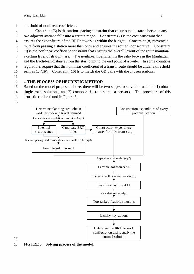
threshold of nonlinear coefficient. 1

Constraint (6) is the station spacing constraint that ensures the distance between any 2

two adjacent stations falls into a certain range. Constraint (7) is the cost constraint that 3

ensures the expenditure of the BRT network is within the budget. Constraint (8) prevents a 4

route from passing a station more than once and ensures the route is consecutive. Constraint 5

(9) is the nonlinear coefficient constraint that ensures the overall layout of the route maintain 6

a certain level of straightness. The nonlinear coefficient is the ratio between the Manhattan 7

and the Euclidean distance from the start point to the end point of a route. In some countries 8

regulations require that the nonlinear coefficient of a transit route should be under a threshold 9

such as 1.4(18). Constraint (10) is to match the OD pairs with the chosen stations. 10

11

4. THE PROCESS OF HEURISTIC METHOD 12

Based on the model proposed above, there will be two stages to solve the problem: 1) obtain 13

single route solutions, and 2) compose the routes into a network. The procedure of this 14

heuristic can be found in Figure 3. 15

16

Determine planning area, obtain

road network and travel demand

Construction expenditure of every

potential station

Construction expenditure

matrix for links from i to j

Feasible solution set I

Feasible solution set II

Feasible solution set III

Nonlinear coefficient constraint (eq.9)

Top-ranked feasible solutions

Calculate served trips

Identify key stations

Potential

stations sites

Candidate BRT

links

Geometric and regelation constraints (eq.1)

Station spacing and consecution constraints (eq.6&eq.8)

Expenditure constraint (eq.7)

Determine the BRT network

configuration and identify the

optimal solution 17

FIGURE 3 Solving process of the model. 18

Wang, Lan, Lian 9

1

Step 0: As described in section 2.3, the distance matrix and the paths between each 2

pair of potential stations are calculated using the Floyd Algorithm. 3

Step 1: If a path goes from i to j via M links, then the Eij can be calculated according 4

to Eq. (11). The expenditure matrix will then be established. The value of cm, which 5

represents the cost per unit length of right of way construction, can be determined according 6

to lane number, length, width, even breadth of the road. 7

8

1

M

ij m m

m

E d c

(11)

9

Step 2: A new matrix with values in 1 or 0 is introduced, which indicates whether two 10

stations can be selected consecutively on a route. The values of the matrix are determined by 11

whether the distance dij of any two potential stations meets the station spacing constraint Eq 12

(6). 13

Step 3: Starting from each potential station, a feasible solution set I is obtained, which 14

contains the routes whose stations can be derived through the 0-1 matrix established in step 2. 15

If a station has already been selected by a route, it will not be selected or passed through 16

again. This ensures that BRT routes meet the route consecution constraint Eq (8). 17

Step 4: Examine the feasible routes generated from Step 3 with respect to cost 18

constraint Eq (7). The feasible solution set II is then obtained, which contains those routes 19

meet station spacing, consecution, and cost constraints. 20

Step 5: Calculate each route’s length and the Euclidean distance between the start 21

station and the end station, and then calculate each route’s nonlinear coefficient. Eliminate 22

the routes whose nonlinear coefficients exceed the threshold, as shown in Eq (9), and obtain 23

the feasible solution set III meeting all constraints. 24

Step 6: Calculate and rank the quantity of direct trips for each feasible route. 25

Step 7: Identify the key stations that frequently appear on the top-ranked feasible 26

routes. 27

Step 8: On the basis of key stations, compose the BRT network configuration by 28

making combinations of the top-ranked routes. Calculate the trips with a transfer, then 29

calculate T(i,j), and finally find the best combination as the optimal solution to the problem. 30

31

5. THE CASE STUDY AND NUMERICAL RESULTS 32

To validate the model and algorithm proposed in this study, Luobei District in the City of 33

Luoyang, China (seeing Figure 4) was chosen for a case study. The road network and travel 34

demand data were obtained from local planning agencies. The data of population, traffic 35

analysis zones and transport network used in this study came from an established travel 36

demand forecast model, which was last updated in 2014. 37

38

Wang, Lan, Lian 10

1

2

FIGURE 4 Case study area of Luoyang, China. 3

4

First, the geometric and regulation constraints are employed to identify the candidate 5

links where BRT right of way can be implemented. Intersections on the candidate links are 6

then numbered as the potential station sites, seeing Figure 5. As shown in the figure, the 7

road network contains 96 links and 65 intersections. 8

9

10

11

FIGURE 5 Candidate links and station sites. 12

13

In the case study, it is assumed lmin =550m, lmax =1,800m, and CN=1.6. Emax are 14

assumed to be a certain budget value according to the number of stations and the total length 15

of a BRT route. The average construction expenditure of a station is assumed to be 1 16

million CNY. 17

Following the steps described in Section 4, more than 100,000 feasible solutions are 18

found till Step 6. In Step 7, station 38, 48, 49 are identified as the key stations because they 19

Wang, Lan, Lian 11

are the most frequently selected ones among the top-ranked feasible solution set. As 1

pointed out by Laporte et al. (9), there are several basic configurations for a transit network 2

including star, cartwheel, triangle, grid and modified configurations. Based on the 3

recommendations and distribution of the key stations, the modified grid configuration is 4

selected for the case study area in order to achieve the best in terms of passenger-network 5

effectiveness. 6

Table 1 and 2 depict the detailed information of the network solution and routes 7

included. Four network options, from a through d, are presented, each having three BRT 8

routes. As shown in Table 1, each route will serve 31,758-35,537 trips directly with length 9

varying from 2,308 to 3,095 meters. The transfer trips are added and shown in Table 2. 10

The expenditure of each route is provided in Table 1 while the total expenditure of each 11

network option is given in Table 2, which indicate the budget constraint Emax is effective. 12

The nonlinear coefficients are under the constraint of 1.6. However, from Figure 6 it can be 13

seen that the alignment of the selected route zigzags in the planning area with the value 14

ranging from 1.49 to 1.58. To improve this, the threshold value of the nonlinear coefficient 15

constraint can be set lower according to the size of the planning area and the number of 16

stations on the BRT route. 17

18

TABLE 1 Summary of the Solutions and Selected Routes 19

20

Option Route

No. Route alignment

Served

OD

Length

(m)

Expenditure

(104 CNY)

Nonlinear

coefficient

a

1 29-27-25-24-23-38-49-48 35,537 3,015 7,888 1.58

2 5-6-15-16-17-50-49-48 33,429 2,308 5,404 1.49

3 42-43-36-22-23-24-49-48 31,758 2,739 6,786 1.55

b

1 18-27-25-23-38-49-48-57 33,660 3,095 8,041 1.54

2 5-6-15-16-17-50-49-48 33,429 2,308 5,404 1.49

3 42-43-36-22-23-24-49-48 31,758 2,739 6,786 1.55

c

1 29-27-25-24-23-38-49-48 35,537 3,015 7,888 1.58

2 60-59-58-48-49-24-23-22 34,703 2,718 6,449 1.55

3 5-6-15-16-17-50-49-48 33,429 2,308 5,404 1.49

d

1 18-27-25-23-38-49-48-57 33,660 3,095 8,041 1.54

2 60-59-58-48-49-24-23-22 34,703 2,718 6,449 1.55

3 5-6-15-16-17-50-49-48 33,429 2,308 5,404 1.49

21

TABLE 2 Summary and Comparison of the Solutions 22

23

Option Directly-served

OD

OD with

Transfer

Objective Function

Value

Total Length

(m)

Expenditure

(104 CNY)

a 100,723 37,462 138,185 8,062 20,078

b 98,847 36,862 134,709 8,143 20,231

c 103,668 47,814 151,482 8,041 19,741

d 101,792 46,702 148,494 8,122 19,894

24

Wang, Lan, Lian 12

1 2

FIGURE 6 Layout of the network solutions. 3

4

From Table 2 it can be seen Option c is better than others in all aspects including the 5

objective function value, the directly-served trips, served trips with transfers, total length and 6

network expenditures. It is then considered the best solution for the case study area with 7

respect to all the constraints. This BRT network option, containing 3 routes, will serve a 8

total of 151,482 direct and one-transfer BRT trips per day in the case study area. It proves 9

that the proposed method is capable of finding the BRT network that will serve the maximum 10

number of OD trips while satisfying the constraints of budget, nonlinear coefficient, 11

minimum and maximum stop distances, and road geometrics. 12

13

6. CONCLUSIONS AND OUTLOOK 14

Considering the factors including distance between stations, expense of construction, road 15

geometrics and so on, the authors proposed a mathematical model for the BRT network 16

planning problem, followed by a heuristic algorithm and a case study in Luoyang, China. 17

The objective function of the model is to maximize the total trips served by a BRT 18

network, subjected to a number of geometric, regulation, station spacing, expenditure, and 19

consecution constraints. Also, nonlinear coefficient is introduced in the mathematical 20

model to measure the straightness of the BRT route alignment. A heuristic method is 21

applied to solve the problem and to generate a BRT network solution. Although the 22

algorithm has relatively low efficiency, it is effective to find the optimal solution of BRT 23

network including routes and stations, and it is easy to understand and implement. 24

This study makes a contribution to improve the scientific and quantitative analysis in 25

BRT planning. Since the planning practice is often influenced by politics and the 26

subjectivity of decision makers, the quantitative results from applying this method can be 27

presented as decision support materials. In the future it is possible to improve the algorithm 28

Wang, Lan, Lian 13

efficiency. The research effort can be further extended to investigate the most efficient 1

network configuration regarding the star, cartwheel, triangle, grid and modified 2

configurations. Also, trips with multiple transfers and the transfer trips between BRT and 3

conventional public transportation system can also be included for calculation to make it 4

close to the real situation. 5

6

REFERENCE 7

1. Levinson, H., Zimmerman, S., Clinger, J., Gast, J., Rutherford, S., & Bruhn, E. 8

Implementation guidelines. Transit Cooperative Research Program - Report 90. In Bus 9

rapid transit, Vol. 2, Transportation Research Board, National Academies, Washington, 10

D.C., 2003. 11

2. Global BRT Data. Produced by Bus Rapid Transit across Latitudes and Cultures and 12

EMBARQ, in partnership with IEA and SIBRT. http://brtdata.org. Accessed June 5, 2016 13

3. Hidalgo, Dario. Bus Rapid Transit, Worldwide History of Development, Key Systems, 14

and Policy Issues. Transportation Technologies for Sustainability. Springer New York, 15

2013, pp. 235-255. 16

4. Lindau, L. A. e D. Hidalgo, et al. Barriers to Planning and Implementing Bus Rapid 17

Transit Systems. Research in Transportation Economics, Vol. 48, 2014, pp.9-15. 18

5. Magnanti, Thomas L., and Richard T. Wong. Network Design and Transportation 19

Planning: Models and Algorithms. Transportation Science. Vol. 18, No. 1, 1984, pp. 20

1-55. 21

6. Guihaire, V. &Hao, J. Transit Network Design and Scheduling: A Global Review. 22

Transportation Research Part A: Policy and Practice, Vol. 42, No. 10, 2008, pp. 23

1251-1273. 24

7. Laporte, G., Mesa, J. A., Ortega, F. A. & Perea, F. Planning Rapid Transit Networks. 25

Socio-Economic Planning Sciences. Vol. 45, No. 3, 2011, pp. 95-104. 26

8. Farahani, R. Z., Miandoabchi, E., Szeto, W. Y. &Rashidi, H. A Review of Urban 27

Transportation Network Design Problems. European Journal of Operational Research. 28

Vol. 229, No. 2, 2013, pp. 281-302. 29

9. Laporte, G., Mesa, J. A. &Ortega, F. A. Optimization Methods for the Planning of Rapid 30

Transit Systems. European Journal of Operational Research, Vol. 122, No. 1, 2000, pp. 31

1-10. 32

10. Gutiérrez-Jarpa, G., Obreque, C., Laporte, G. &Marianov, V. Rapid Transit Network 33

Design for Optimal Cost and Origin–Destination Demand Capture. Computers & 34

Operations Research, Vol. 40, No. 12, 2013, 3000-3009. 35

11. Bruno, G., Gendreau, M. &Laporte, G. A Heuristic for the Location of a Rapid Transit 36

Line. Computers & Operations Research, Vol. 29, No. 1, 2002, pp. 1-12. 37

12. Nikolić, M. &Teodorović, D. Transit Network Design by Bee Colony Optimization. 38

Expert Systems with Applications, Vol. 4, No. 15, 2013, 5945-5955. 39

13. Nayeem, M. A., Rahman, M. K. &Rahman, M. S. Transit network design by genetic 40

algorithm with elitism. Transportation Research Part C: Emerging Technologies 46, 41

2013, pp. 30-45. 42

14. Hosapujari, A. B. &Verma, A. Development of a Hub and Spoke Model for Bus Transit 43

Route Network Design. Procedia - Social and Behavioral Sciences, Vol. 104, No. 1, 44

Wang, Lan, Lian 14

2013, pp. 835-844. 1

15. The setting for bus lanes. Ministry of Public Security, the People's Republic of China, 2

2004. 3

16. Gutiérrez-Jarpa, G. e C. Obreque, et al. Rapid Transit Network Design for Optimal Cost 4

and Origin–Destination Demand Capture. Computers & Operations Research, Vol.40, 5

No.12, 2013, p.3000-3009. 6

17. Tsinghua University Press, Theory and Method in Transportation Planning (Second 7

Editon ). Lu Huapu. Beijing, 2006. 8

18. Code for transport planning on urban road. State bureau of technical supervision, the 9

ministry of construction of the People's Republic of China, 1995. 10