1

2

Two-samples tests, X2

Dr. Mona Hassan AhmedProf. of Biostatistics

HIPH, Alexandria University

3

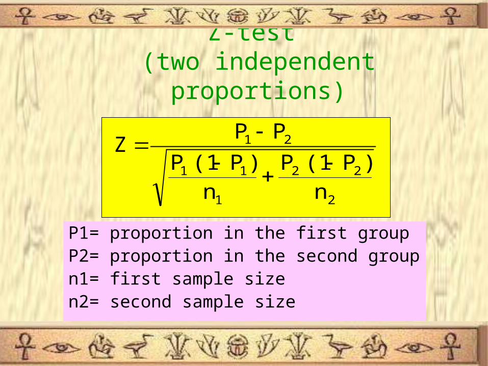
Z-test (two independent proportions)

P1= proportion in the first groupP2= proportion in the second group n1= first sample sizen2= second sample size

2

22

1

11

21

n)P(1 P

n)P(1 P

PPZ

4

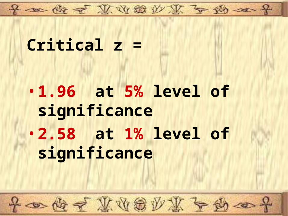
Critical z =

• 1.96 at 5% level of significance

• 2.58 at 1% level of significance

5

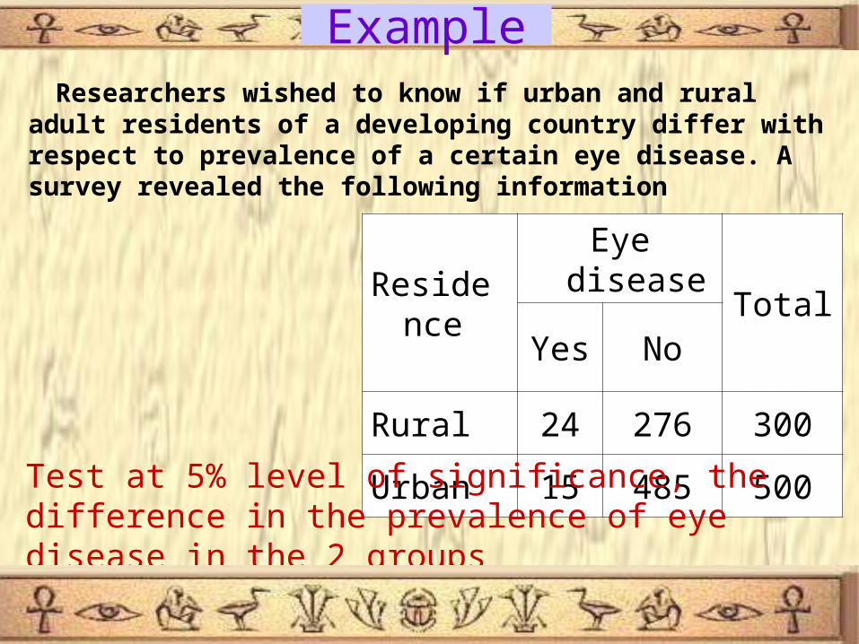
Researchers wished to know if urban and rural adult residents of a developing country differ with respect to prevalence of a certain eye disease. A survey revealed the following information

ResidenceEye disease

TotalYes No

Rural 24 276 300

Urban 15 485 500

Test at 5% level of significance, the difference in the prevalence of eye disease in the 2 groups

Example

6

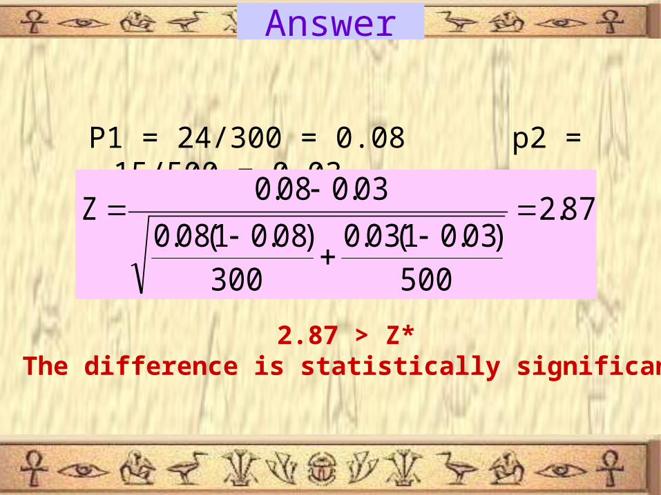
P1 = 24/300 = 0.08 p2 = 15/500 = 0.03

87.2

500)03.01(03.0

300)08.01(08.0

03.008.0Z

2.87 > Z* The difference is statistically significant

Answer

7

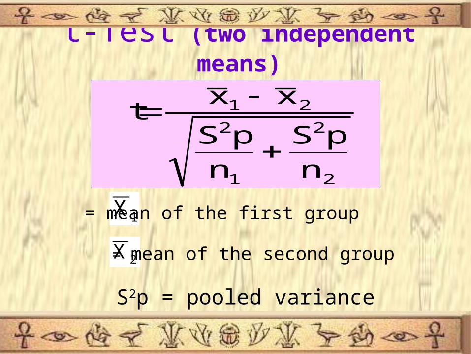
t-Test (two independent means)

2

2

1

2

21

npS

npS

xx t

1X = mean of the first group

2X = mean of the second group

S2p = pooled variance

8

2nn

1)S(n1)S(nPS

21

22

212

12

Critical t from table is detected at degree of freedom = n1+ n2 - 2 level of significance 1% or 5%

9

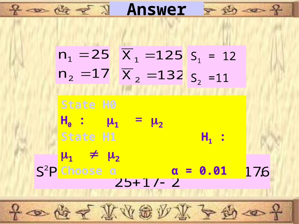
Sample of size 25 was selected from healthy population, their mean SBP =125 mm Hg with SD of 10 mm Hg . Another sample of size 17 was selected from the population of diabetics, their mean SBP was 132 mmHg, with SD of 12 mm Hg .

Test whether there is a significant difference in mean SBP of diabetics and healthy individual at 1% level of significance

Example

10

17n

25n

2

1

132X

125X

2

1

S1 = 12

S2 =11

6.11721725

1)12(171)10(25PS

222

State H0 H0 : 1 = 2

State H1 H1 : 1 2

Choose α α = 0.01

Answer

11

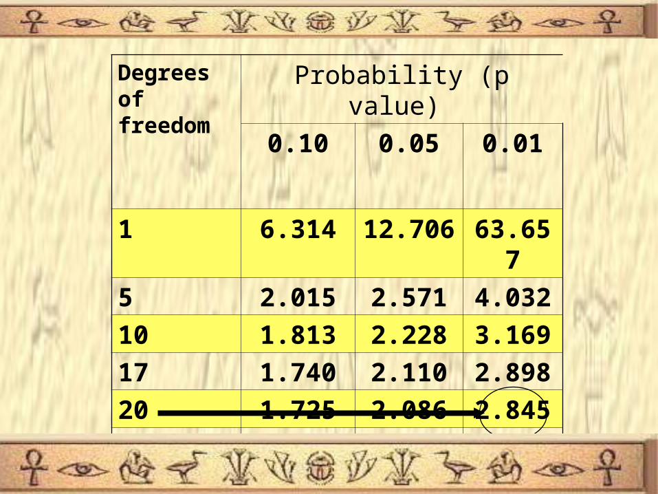
Critical t at df = 40 & 1% level of significance = 2.58

2.503

17117.6

25117.6

132125t

Decision:Since the computed t is smaller than critical t so there is no significant difference between meanSBP of healthy and diabetic samples at 1 %.

Answer

12

Degrees of freedom

Probability (p value)

0.10 0.05 0.01

1 6.314 12.706 63.657

5 2.015 2.571 4.032

10 1.813 2.228 3.169

17 1.740 2.110 2.898

20 1.725 2.086 2.845

24 1.711 2.064 2.79725 1.708 2.060 2.787

1.645 1.960 2.576

13

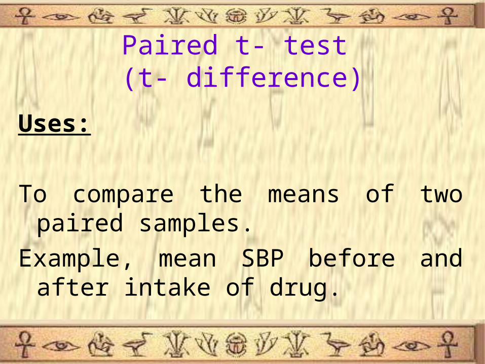
Paired t- test (t- difference)

Uses:

To compare the means of two paired samples.

Example, mean SBP before and after intake of drug.

14

di = difference (after-before)Sd = standard deviation of difference n = sample size Critical t from table at df = n-1

n

Sdd

t

1nn

di)(di

Sd

22

differencemean

n

did

15

The following data represents the

reading of SBP before and after

administration of certain drug. Test

whether the drug has an effect on

SBP at 1% level of significance.

Example

16

Serial No.SBP

(Before)SBP

(After)

1 200 180

2 160 165

3 190 175

4 185 185

5 210 170

6 175 160

17

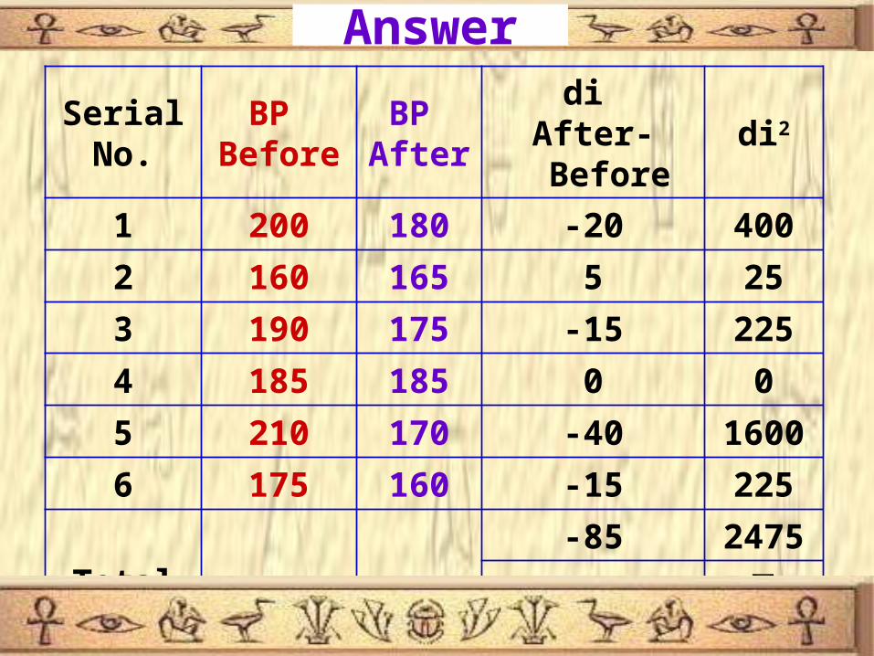
SerialNo.

BP Before

BP After

di After-Before

di2

1 200 180 -20 400

2 160 165 5 25

3 190 175 -15 225

4 185 185 0 0

5 210 170 -40 1600

6 175 160 -15 225

Total-85 2475

∑di ∑ di2

Answer

18

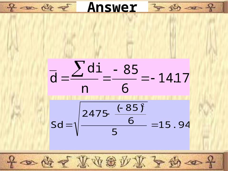
17.146

85

n

did

15.9425

6

85)(2475

Sd

2

Answer

19

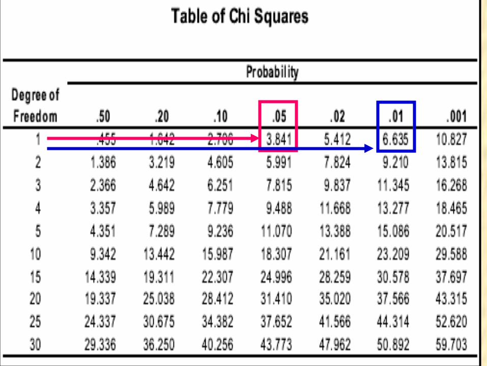
Critical t at df = 6-1 = 5 and 1% level of significance

= 4.032

Decision:

Since t is < critical t so there is no significant difference between mean SBP before and after administration of drug at 1% Level.

2.17

6

15.94214.17

tComputed

Answer

20

Degrees of freedom

Probability (p value)

0.10 0.05 0.01

1 6.314 12.706 63.657

5 2.015 2.571 4.032

10 1.813 2.228 3.169

17 1.740 2.110 2.898

20 1.725 2.086 2.845

24 1.711 2.064 2.79725 1.708 2.060 2.787

1.645 1.960 2.576

21

Chi-Square test

It tests the association between variables... The data is qualitative .

It is performed mainly on frequencies.

It determines whether the observed frequencies differ significantly from expected frequencies.

22

Where E = expected frequency O = observed frequency

i

2

ii2

E

)E(OΧComputed

totalGrand

alColumn tot totalRawE

23

Critical X2 at df = (R-1) ( C -1) Where R = raw C = column

I f 2 x 2 table

X2* = 3.84 at 5 % level of significance

X2* = 6.63 at 1 % level of significance

24

25

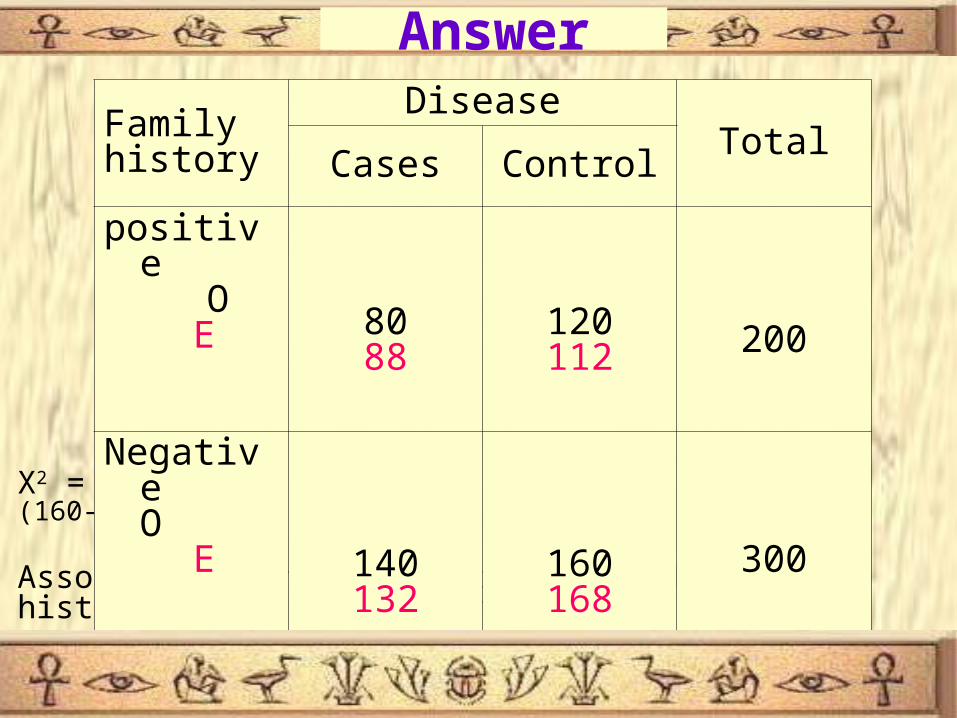
In a study to determine the effect of heredity in a certain disease, a sample of cases and controls was taken:

Family history

DiseaseTotal

Cases Control

Positive 80 120 200

Negative 140 160 300

Total 220 280 500Using 5% level of significance, test whether family history has an effect on disease

Example

26

X2 = (80-88)2/88 + (120-112)2/112 + (140-132)2/132 + (160-168)2/168 = 2.165 < 3.84Association between the disease and family history is not significant

Family history

DiseaseTotal

Cases Control

positive O

E

8088

120112 200

Negative O

E

140132

160168

300

Total 220 280 500

Answer

27

• The odds ratio was developed to quantify exposure – disease relations using case-control data

• Once you have selected cases and controls ascertain exposure

• Then, cross-tabulate data to form a 2-by-2 table of counts

28

2-by-2 Crosstab Notation Disease + Disease - Total

Exposed + A B A+B

Exposed - C D C+D

Total A+C B+D A+B+C+D

• Disease status A+C = no. of cases B+D = no. of non-cases

• Exposure status A+B = no. of exposed individuals C+D = no. of non-exposed individuals

29

Disease + Disease -

Exposed + A B

Exposed - C D

BC

ADOR

C

Ao 1 cases odds, exposure

D

Bo 0 controls odds, exposure

BC

AD

DB

CA

o

oOR

/

/ratio odds

0

1

Cross-product

ratio

30

• Exposure variable = Smoking

• Disease variable = Hypertension

D+ D-

E+ 30 71

E- 1 22

Total 31 93

3.9)1)(71(

)22)(30(

BC

ADOR

Example

31

Interpretation of the Odds Ratio

• Odds ratios are relative risk estimates

• Relative risk are risk multipliers

• The odds ratio of 9.3 implies 9.3× risk with exposure

32

No association

OR < 1

OR = 1

OR > 1Positive association

Higher risk

Negative associationLower risk (Protective)

33

• In the previous example

OR = 9.3

• 95% CI is 1.20 – 72.14

34

Multiple Levels of Exposure

Smoking level Cases Controls

Heavy smokers 213 274

Moderate smokers 61 147

Light smokers 14 82

Non-smokers 8 115

Total 296 618

35

Multiple Levels of Exposure

• k levels of exposure break up data into (k – 1) 22 tables

• Compare each exposure level to non-exposed • e.g., heavy smokers vs. non-smokers

Cases Controls

Heavy smokers 213 274

Non-smokers 8 1152.11

)8)(274(

)115)(213(OR

36

Multiple Levels of Exposure

Smoking level Cases Controls

Heavy smokers 213 274 OR3 =(213)(115)/(274)(8)=11.2

Moderate smokers 61 147 OR2 =(61)(115)/(147)(8) = 6.0

Light smokers 14 82 OR1 =(14)(115)/(82)(8) = 2.5

Non-smokers 8 115

Total 605 115

Notice the trend in OR

(dose-response relationship)

37

Small Sample Size Formula For the Odds Ratio

It is recommend to add ½ to each cell before calculating the odds ratio when some cells are zeros

D+ D-

E+ 31 71

E- 0 22

Total 31 93

OR Small Sample =(A+0.5)(D+0.5)

(B+0.5)(C+0.5)

OR Small Sample =(31+0.5)(22+0.5)

=19.8(71+0.5)(0+0.5)

38