1

2

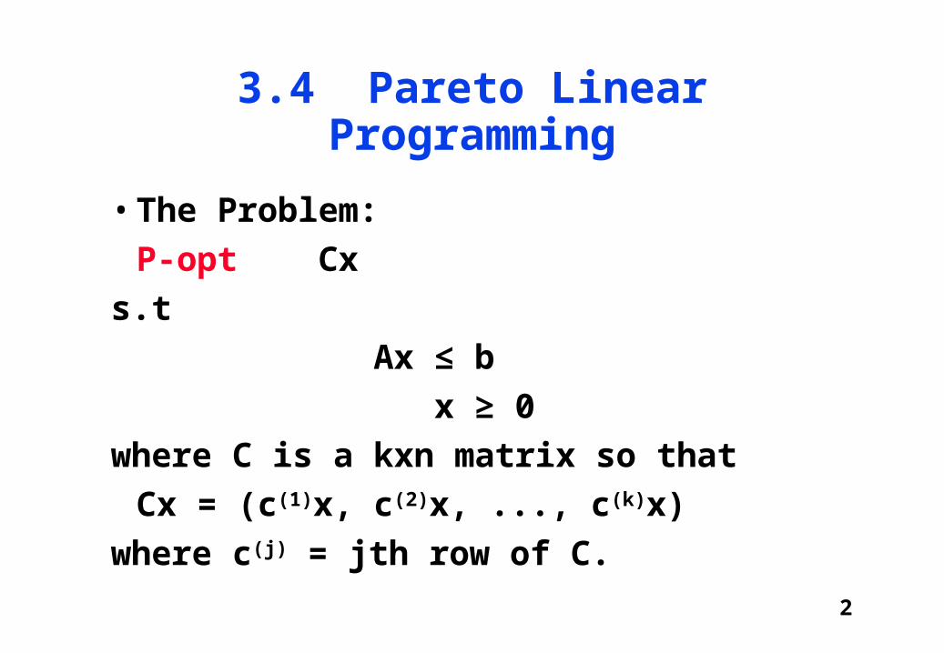
3.4 Pareto Linear Programming

• The Problem:

P-opt Cx

s.t

Ax ≤ b

x ≥ 0

where C is a kxn matrix so that

Cx = (c(1)x, c(2)x, ..., c(k)x)

where c(j) = jth row of C.

3

Example

• P- max {3x1 + 2x2, 2x1 – x2}

• S.t.

• x1 ≤ 2

• 3x1 + x2 ≤ 9

• x1, x2 ≥ 0

Here z = (z1, z2).

z1 z2

4

• We refer to the Pareto solutions also as efficient points, or non-dominated points.

• We shall focus on opt = max.

• For simplicity we shall assume that the set of feasible solution, namely

X := {x in Rn: Ax ≤ b, x ≥ 0}

is bounded.

• Let

Z:= {Cx: x in X}

observing that Z is a subset of Rk, and usually k <<<<<n.

5

6

We can solve for the efficient points graphically if we only have 2 variables and 2 objective functions.This also gives us a good picture of what is going on, and ideas for generalizing.

• P- max {3x1 + 2x2, 2x1 – x2}

• S.t.

• x1 ≤ 2

• 3x1 + x2 ≤ 9

• x1, x2 ≥ 0

7

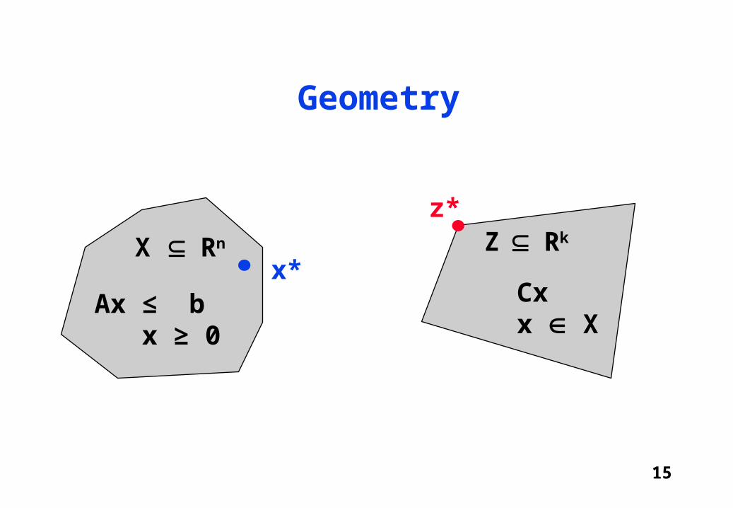
So more generally: Geometry

Ax ≤ b x ≥ 0

X Rn Z Rk

Cxx X

8

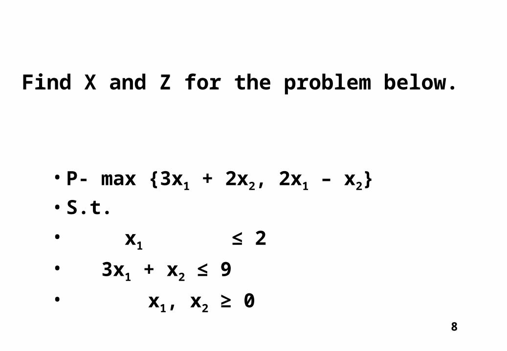
• P- max {3x1 + 2x2, 2x1 – x2}

• S.t.

• x1 ≤ 2

• 3x1 + x2 ≤ 9

• x1, x2 ≥ 0

Find X and Z for the problem below.

9

How do we generate all the Pareto Solutions?

• Idea:

• Generate the non-dominated extreme points of Z

• Use them to generate the other efficient points of Z.

• Rationale:

• Other efficient points of Z are convex combinations of the efficient extreme points of Z

10

k=2 (i.e 2-objectives)

z2

z1

11

k=2

z2

z1

Z

12

k=2

z2

z1

Z

Efficient points(Pareto solutions)

13

k=2

z2

z1

Z

Efficient points

Efficient extremepoints

Every efficient point can be expressed as a convex combination of the efficient extreme points. So we first aim to generate the efficient extreme points.

14

An extremely important theorem

• Idea:

• Theorem 4.6.1

• An extreme point of Z must be produced by an extreme point of X, ie if z* is an extreme point of Z then z*=Cx* where x* is an extreme point of X

• Proof:

• By contradiction. Assume that z* is an extreme point of Z but x* in X for which z*=Cx*, is not an extreme point of X.

15

Geometry

Ax ≤ b x ≥ 0

X Rn Z Rk

Cxx X

x*

z*

16

• Since x* is not an extreme point of X we have

x* = x’ + (1-)x” , 0 < < 1

for some points x’ and x” in X.

Thus,

z* = Cx* = C(x’ + (1-)x”)

= Cx’ + (1-)Cx”

= z’ + (1-)z” ,

(z’=Cx’, z”=Cx”)

This, however, contradicts the assertion that z* is an extreme point of Z.

(This is true only when z’ and z” are different and neither of z’ and z” is an extreme point)

17

Comment

Ax ≤ b x ≥ 0

X Rn Z Rk

Cxx X

x*

z*

If z* extreme then x* extreme.BUT not necessarily vice versa.

18

19

• One way to generate the efficient extreme points of Z is by deploying the following well known results:

• Theorem 4.6.2:

• If z* is an efficient point of Z then there must be a in Rk such that z* is an optimal solution to the problem:

• max { z: z in Z} (****)

i.e. max {z1+ z2+…+ zk : z in Z}

• Furthermore, > 0 (all components are strictly positive)

20

Theorem 4.6.3:

If > 0 then any optimal solution to

max {z1+ z2+…+ zk : z in Z} (****)

is an efficient point of Z.

21

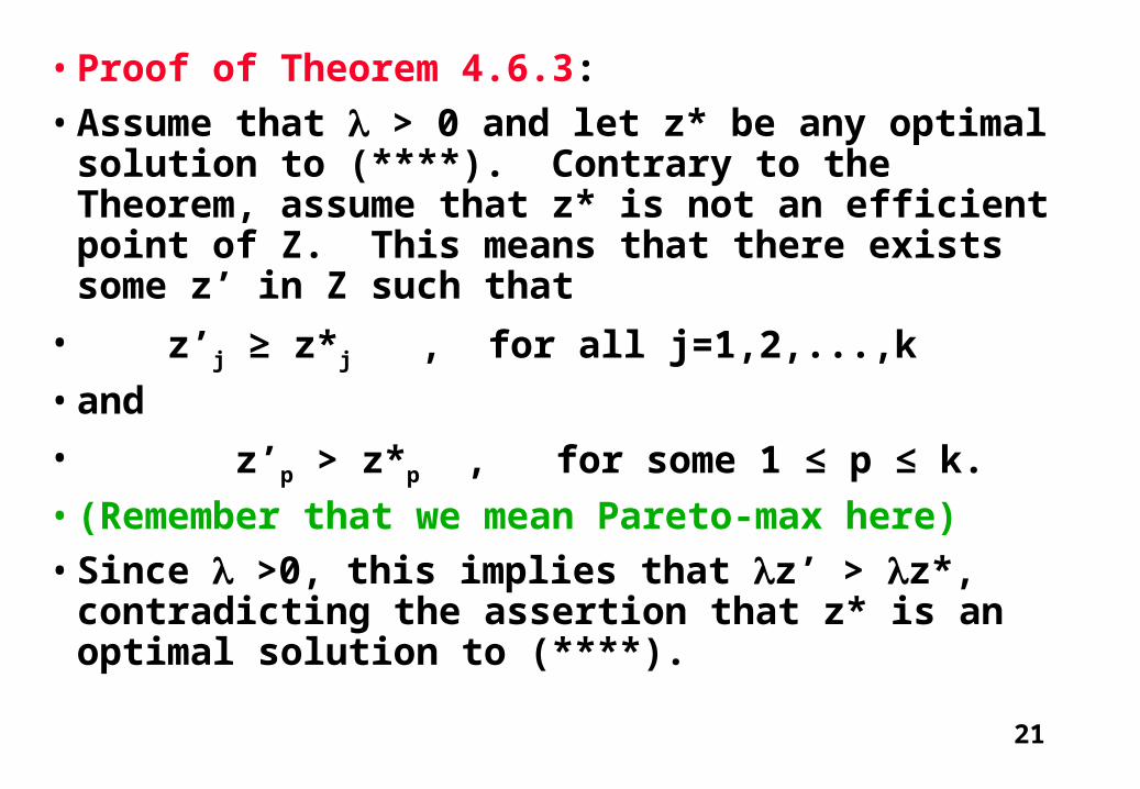
• Proof of Theorem 4.6.3:

• Assume that > 0 and let z* be any optimal solution to (****). Contrary to the Theorem, assume that z* is not an efficient point of Z. This means that there exists some z’ in Z such that

• z’j ≥ z*j , for all j=1,2,...,k

• and

• z’p > z*p , for some 1 ≤ p ≤ k.

• (Remember that we mean Pareto-max here)

• Since >0, this implies that z’ > z*, contradicting the assertion that z* is an optimal solution to (****).

22

• Understanding Theorem 4.6.2 requires some fundamental results!!!

• We will omit slides 17 - 40 (not examinable).

• From slide 41 on is examinable.

23

Review(618-261)

• Convex set:

• If y’ and y” are elements of Y then the entire line segment connecting these points is also in Y.

• Line segment:

• Line segment connecting y’ and y” is the set of all the convex combinations of y’ and y”.

• Convex combinations:

• y =y’ + (1-)y” , 0 ≤ ≤ 1.

24

25

X1X2

X1X2

X1X2

Convex comb. of X1 and X2

Not convex comb. of X1 and X2

Extreme Points

• A point y in Y is an extreme point of Y if it cannot be expressed as a convex combination of two other points in Y.

26

2 extreme points

4 extreme points(the corners)

Entire boundary is extreme

27

Properties of Convex Sets

• If S is a convex set, then for any in R+,

S := {s: s in S}

is a convex set.

• If S and T are convex sets, then so is

S + T : = {s+t: s in S, t in T}

• The intersection of any collection of convex sets is convex.

28

origin

S

S

ST

S+TA

B

29

facts about hyperplanes

• Fact 1:

• Let be a non-zero element of Rn and let b be a real number. Then the set

H := {x in Rn: x = b}

is a hyperplane in Rn.

• Example:

• In R3, the set of all points satisfying

3x1 + 3x2 + x3 =5

is a hyperplane (set b=5 and = (3,3,1) )

30

• Fact 2:

• Let H be a hyperplane in Rn. Then there is a non-zero vector in Rn and a constant b such that

• H = S:= {x in Rn: x=b}.

31

bottom line

• A hyperplane in Rn is the set of solutions to a single linear equation.

32

Half Spaces

• Given a hyperplane, say

H := {x in Rn : x = b}

we shall consider the two closed half spaces it generates:

H+ := {x in Rn: x ≥ b}

H– := {x in Rn: x ≤ b}

33

H+

H–

H := {x in Rn: x=b}

34

Main Results(for our purposes)

• Theorem 4.6.4 Separating Hyperplanes

• Given a convex set S and a point x exterior to its closure*, there is a hyperplane containing x that contains S in one of its half spaces.

• Closure of S: the smallest closed set containing S.

• Closed set: A set with the property that any point that is arbitrarily close to it is a member of the set.

35

S

Hx

36

SH

x

x

S

37

• Theorem 4.6.5 Supporting Hyperplane

• Let S be a convex set and let x be a boundary point of S. Then there is a hyperplane containing x and containing S in one of its closed half spaces.

SSupporting hyperplane at x

x

38

• Theorem 4.6.6

• Let S be a convex set, H a supporting hyperplane of S and I the intersection of H and S.

• Then every extreme point of I is an extreme point of S.

39

One common extreme point

SH

I

S

H

I

two extreme points in common

Face

Facet

40

And so ......• For every extreme point in Z there is a

supporting hyperplane

• Each extreme point of Z is an optimal solution to max {z : z in Z} for some non zero in Rk.

41

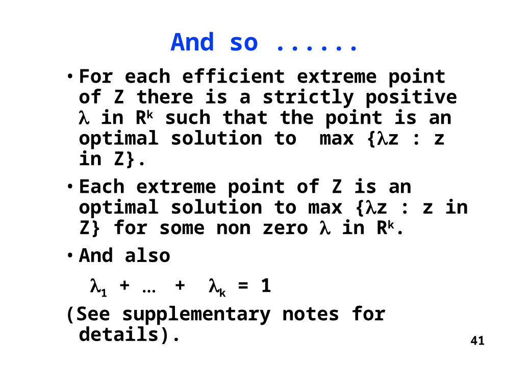
And so ......• For each efficient extreme point of Z

there is a strictly positive in Rk such that the point is an optimal solution to max {z : z in Z}.

• Each extreme point of Z is an optimal solution to max {z : z in Z} for some non zero in Rk.

• And also

1 + + k = 1

(See supplementary notes for details).

42

43

Bottom line• We can generate the efficient extreme

points associated with

P-opt Cx

Ax ≤ b

x ≥ 0

by solving

max Cx

Ax ≤ b

x≥ 0

for all .

44

ExampleP−max{ 3x + x + 4x3 , x + 4x +3x3}

s.t.x + 3x + 5x3 ≤9

8x + 5x + x3 ≤79x + x + 4x3 ≤6

x + 5x + 3x3 ≤8x,x ,x3 ≥

45

• k=2

• Thus we need two multipliers 1 and 2.

• The objective function of the parametric linear programming problem will therefore be of the form:

z() := 1c(1)x + 2c(2)x

• But since the parameters are positive, we can divide say by 1, so obtain an equivalent objective function of the form

z() := c(1)x + c(2)x , =2 / 1

The parametric problem is thus:

C =3 44 3

⎡⎣⎢

⎤⎦⎥

46

• Note that varies from 0 to infinity but cannot equal 0.

max{3x1 + x + 4x3 +(x + 4x + 3x3)}s.t.

x + 3x + 5x3 ≤9

8x + 5x + x3 ≤79x + x + 4x3 ≤6

x + 5x + 3x3 ≤8x,x ,x3 ≥

47

z2

z1

Z

Efficient points

Efficient extremepoints

48

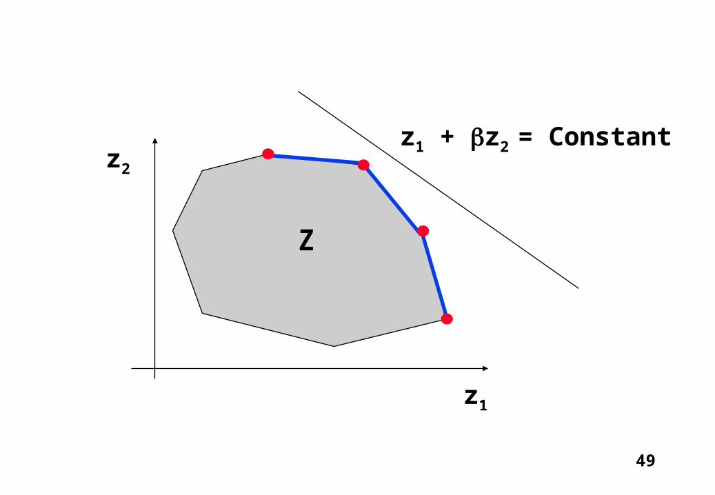
z2

z1

Z

49

z2

z1

Z

z1 + z2 = Constant

50

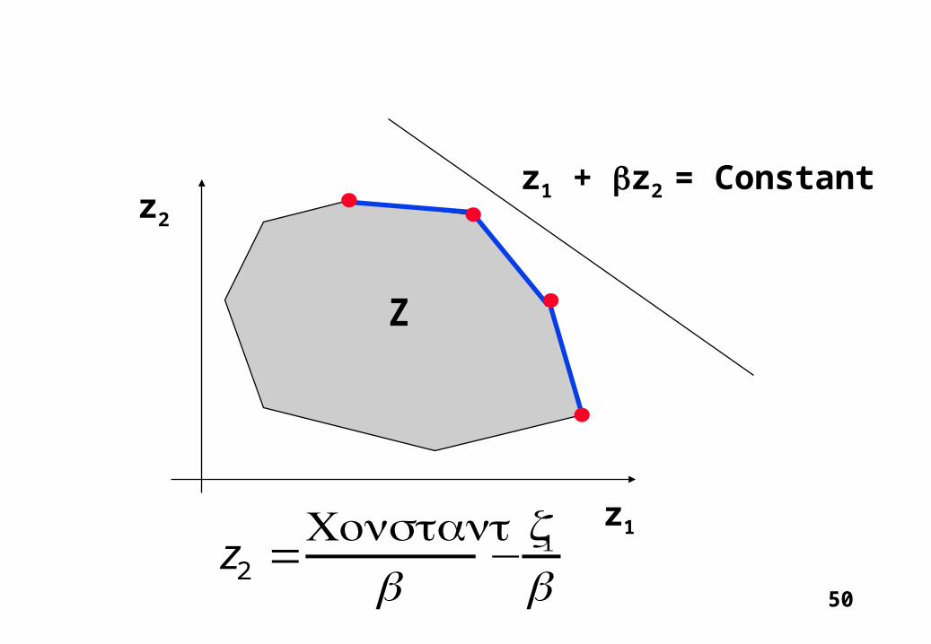
z2

z1

Z

z1 + z2 = Constant

z2 =Constant

−z

51

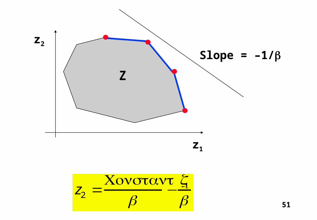
z2

z1

Z

Slope = –1/

z2 =Constant

−z

52

z2

z1

Z

Slope = 0

53

z2

z1

Z

54

z2

z1

Z

55

z2

z1

Z

56

z2

z1

Z

57

z2

z1

Z

58

z2

z1

Z

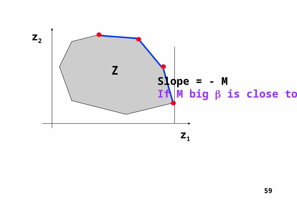
59

z2

z1

ZSlope = - MIf M big is close to 0.

60

Comments

• Read 618-261 Lecture Notes (Chapter 8) regarding changes in the objective function.

• In particular, changes to the cost coefficient of a basic variable (Why?)

• Check your result: We know something about the optimal values of the objective function as changes.

61

Parametric Linear Programming(Objective function)

• Set up:

• z*() := opt z():=c()x , 0 < < s.t.

Ax ≤ b

x ≥ 0

We want to generate the optimal solution x* as a function of the parameter . Symbolically we write it x*().

62

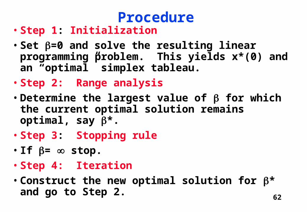
Procedure• Step 1: Initialization

• Set =0 and solve the resulting linear programming problem. This yields x*(0) and an “optimal” simplex tableau.

• Step 2: Range analysis

• Determine the largest value of for which the current optimal solution remains optimal, say *.

• Step 3: Stopping rule

• If = stop.

• Step 4: Iteration

• Construct the new optimal solution for * and go to Step 2.

63

Details

• Step 2: Range analysis

• This is done in the usual manner (618-261 chapter 8) using the optimality test for the reduced costs.

• Step 4: Iteration

• This involves the usual pivot operation which produces an adjacent extreme point (exchange of one basic and one non-basic variable).

64

Example

• Find all the Pareto extreme points of the following problem:

P− {max3x + 5x,x −x}s.t.x ≤4

x ≤3x + x ≤8

x,x ≥

65

To do this we solve

z* ( ):max{(3 2 )x1 (5 )x2

s.t.

x1 4

2x2 12

3x1 2x218

x1, x

2 0

}, for all >0.

z* () := {max3x + 5x +(x −x )}i.e.

(Hillier and Lieberman p. 308)

66

Step 1: initialization

• For =0 the objective function is z(0)=3x1+5x2.

• We solve the problem for this objective function in the usual (simplex) manner.

67

Final Tableau=0

x1 x2 x3 x4 x5 RHS x3 0 0 1 1/3 -1/3 2x2 0 1 0 0.5 0 6x1 1 0 0 -1/3 1/3 2Z 0 0 0 1.5 1 36

X1 = 2, X2 = 6x*(0) = (2,6)z*(0) = 36

68

Step 2: Range analysis

• We now increase from zero until a new (adjacent) optimal solution is generated.

• We determine the critical value of , call it * by introducing in the z-row of the final tableau.

• This typically involves solving a system of simple (range) inequalities (requiring the reduced costs to be non-negative).

69

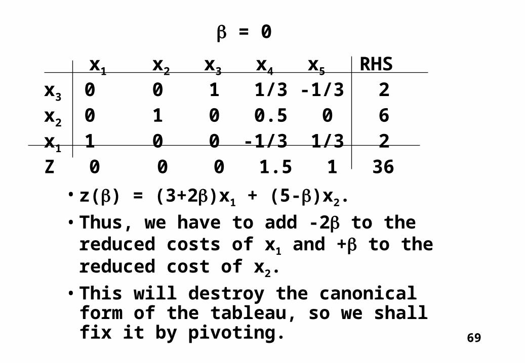
• z() = (3+2)x1 + (5-)x2.

• Thus, we have to add -2 to the reduced costs of x1 and + to the reduced cost of x2.

• This will destroy the canonical form of the tableau, so we shall fix it by pivoting.

x1 x2 x3 x4 x5 RHS x3 0 0 1 1/3 -1/3 2x2 0 1 0 0.5 0 6x1 1 0 0 -1/3 1/3 2Z 0 0 0 1.5 1 36

= 0

70

• To restore the canonical form we have to fix the z-row (2 pivot operations)

x1 x2 x3 x4 x5 RHS x3 0 0 1 1/3 -1/3 2x2 0 1 0 0.5 0 6x1 1 0 0 -1/3 1/3 2Z -2 0 1.5 1 36

71

• This tableau is optimal if

1.5 - 7/6 ≥ 0 (and 1+ 2/3≥0)I.e if 0 ≤ ≤ 9/7• yielding *=9/7.

• X*((2,6), z*(36-20 ≤ ≤ 9/7.

x1 x2 x3 x4 x5 RHS x3 0 0 1 1/3 -1/3 2x2 0 1 0 0.5 0 6x1 1 0 0 -1/3 1/3 2Z 0 0 (1.5-7/6) (1+ 2/3) 36-2

72

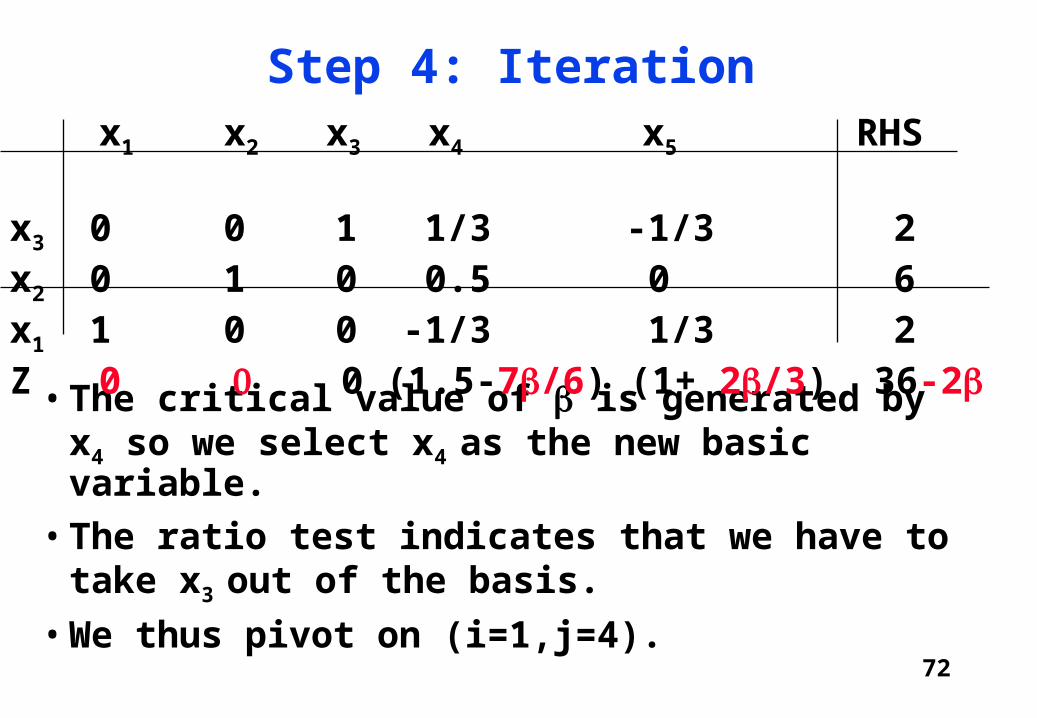
Step 4: Iteration

• The critical value of is generated by x4 so we select x4 as the new basic variable.

• The ratio test indicates that we have to take x3

out of the basis.

• We thus pivot on (i=1,j=4).

x1 x2 x3 x4 x5 RHS x3 0 0 1 1/3 -1/3 2x2 0 1 0 0.5 0 6x1 1 0 0 -1/3 1/3 2Z 0 0 (1.5-7/6) (1+ 2/3) 36-2

73

• So now we repeat the iteration in the context of the new basic solution.

x1 x2 x3 x4 x5 RHS x4 0 0 3 1 -1 6x2 0 1 -3/2 0 0.5 3x1 1 0 0 0 0 4Z 0 0 (-9/2+7/2) 0 (2.5-/2) (27+5

This is optimal if -9/2+7/2 ≥ 0 and 2.5-/2≥ 0i.e. 9/7≤ ≤5, x*( = (4,3), z* *( = (27 + 5 * = 5.

74

Step 4: Iteration

• the variable yielding the critical value of is x5 thus we enter x5 into the basis.

• the ratio test indicates that we take x2 out of the basis.

• Thus, we pivot on (i=2,j=5).

x1 x2 x3 x4 x5 RHS x4 0 0 3 1 -1 6x2 0 1 -3/2 0 0.5 3x1 1 0 0 0 0 4Z 0 0 (-9/2+7/2) 0 (2.5-/2) (27+5

75

• This is optimal if ≥ 5.

• X* ( =(4,0), z* ( =12 +8*= • Stop.

• The extreme points are x = (2,6), (4,3), (4,0) and corresponding efficient extreme points are (36, -2), (27, 5), (12, 8) .

x1 x2 x3 x4 x5 RHS x4 0 2 0 1 0 2x5 0 2 -3 0 1 6x1 1 0 1 0 0 4Z 0 -5+ 3+2 0 0 12+8

76

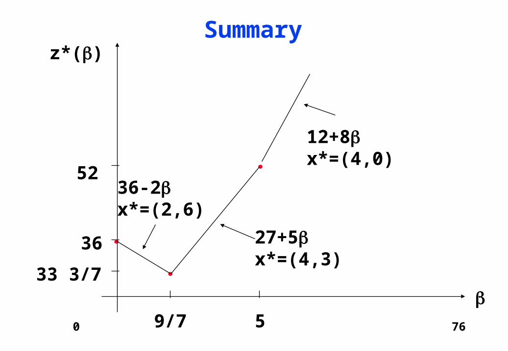
Summary

0

z*()

36

9/7

33 3/7

5

5236-2x*=(2,6)

27+5x*=(4,3)

12+8x*=(4,0)

77

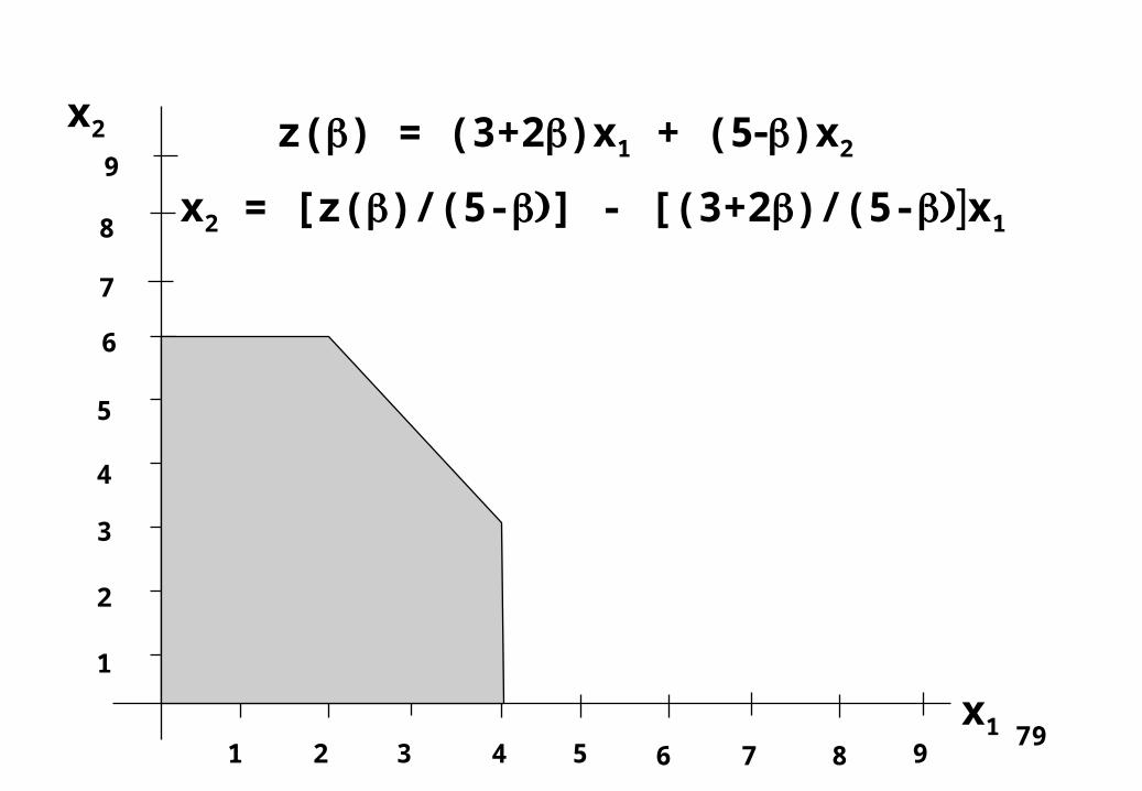
Geometry

z* ():=max(3 + )x + (5−)xs.t.

x ≤4x ≤

3x + x ≤8x,x ≥

78

x2

x1

1

2

3

4

5

1 2 3 4 5 6 7 8 9

6

7

8

9

Feasible set

79

x2

x1

1

2

3

4

5

1 2 3 4 5 6 7 8 9

6

7

8

9z() = (3+2)x1 + (5)x2

x2 = [z()/(5-] - [(3+2)/(5-x1

80

x2

x1

1

2

3

4

5

1 2 3 4 5 6 7 8 9

6

7

8

9z() = (3+2)x1 + (5)x2

x2 = [z()/(5-] - [(3+2)/(5-x1

81

x2

x1

1

2

3

4

5

1 2 3 4 5 6 7 8 9

6

7

8

9z() = 3x1 + 5x2

x2 = (z()/5) - (3/5)x1

82

x2

x1

1

2

3

4

5

1 2 3 4 5 6 7 8 9

6

7

8

9z() = 7x1 + 3x2

x2 = [z()/3] - (7/3)x1

83

x2

x1

1

2

3

4

5

1 2 3 4 5 6 7 8 9

6

7

8

9z(5) = 13x1

84

Some Results

• Consider the parametric problem:

L() := max {f(x) + g(x): x in X}, in R

• Theorem:

The set of ’s for which the same x in X is optimal is convex.

Theorem:

Then, L() is convex with . Furthermore, if there are finitely many optimal solutions, then, L() is piecewise linear.

85

for in R, X is discrete

L() := max {f(x) + g(x): x in X}, in R

L()

The same x is optimalfor all in this range