Problem: An object is shot upwards with an initial velocity of v0 m/s. Its height h

(in m) after t seconds is given by

where r is a drag coefficient and g is 9.81 m/s2.

If r = 0.35 s-1 and v0 = 78 m/s

(i) When will be object be 80m above the ground?

(ii) When will the object hit the ground?

(iii) What maximum height will be attained?

( )r

gte

r

gv

rh rt −−

+= −11

0

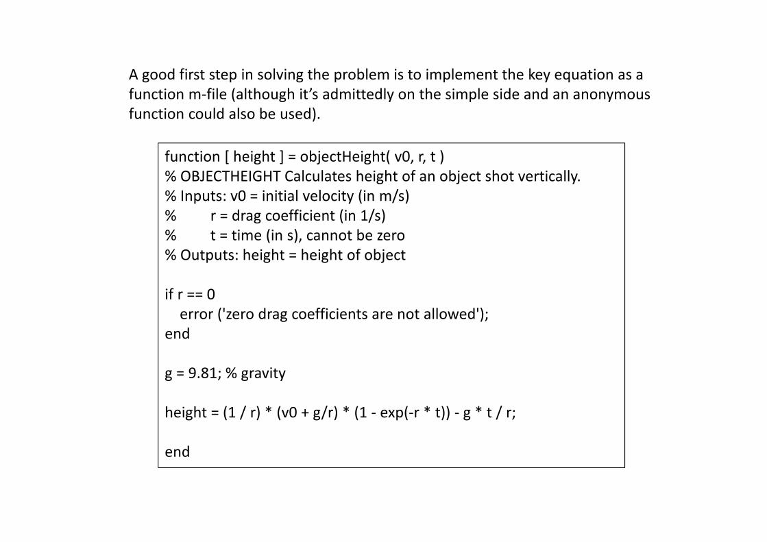
function [ height ] = objectHeight( v0, r, t )

% OBJECTHEIGHT Calculates height of an object shot vertically.

% Inputs: v0 = initial velocity (in m/s)

% r = drag coefficient (in 1/s)

% t = time (in s), cannot be zero

% Outputs: height = height of object

if r == 0

error ('zero drag coefficients are not allowed');

end

g = 9.81; % gravity

height = (1 / r) * (v0 + g/r) * (1 - exp(-r * t)) - g * t / r;

end

A good first step in solving the problem is to implement the key equation as a

function m-file (although it’s admittedly on the simple side and an anonymous

function could also be used).

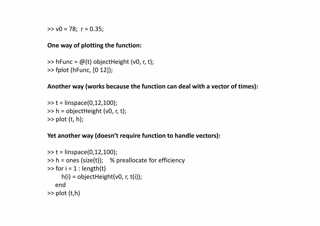
>> v0 = 78; r = 0.35;

One way of plotting the function:

>> hFunc = @(t) objectHeight (v0, r, t);

>> fplot (hFunc, [0 12]);

Another way (works because the function can deal with a vector of times):

>> t = linspace(0,12,100);

>> h = objectHeight (v0, r, t);

>> plot (t, h);

Yet another way (doesn’t require function to handle vectors):

>> t = linspace(0,12,100);

>> h = ones (size(t)); % preallocate for efficiency

>> for i = 1 : length(t)

h(i) = objectHeight(v0, r, t(i));

end

>> plot (t,h)

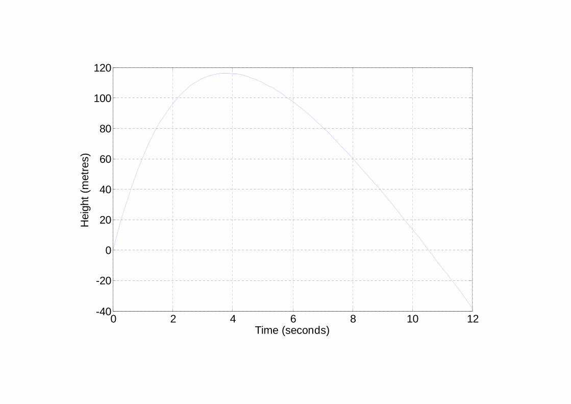
0 2 4 6 8 10 12-40

-20

0

20

40

60

80

100

120

Time (seconds)

Hei

ght

(met

res)

Part (i) solution:

>> f = @(t) objectHeight(v0, r, t) - 80;

>> time1 = fzero (f, [0 2])

time1 =

1.4520

>> time2 = fzero (f, [6, 8])

time2 =

7.0315

Part (ii) solution:

>> f = @(t) objectHeight(v0, r, t);

>> time3 = fzero (f, [10, 12])

time3 =

10.5378

Part (iii) requires new techniques.

One possibility is to differentiate the height equation and set the result equal to

zero.

This reduces the problem to a root finding exercise:

>> g = 9.81; % previously only defined in function

>> der = @(t) (1 / r) * (v0 + g/r) * (r * exp(-r * t)) - g / r;

>> tmax = fzero (der, [3 5])

t max=

3.8014

>> maxHeight = objectHeight (v0, r, tmax)

maxHeight =

116.3098

Note: In general a point at which the derivative is zero can be either a minimum, a

maximum, or an inflection point. In this case our plot makes the situation clear.

( )r

gre

r

gv

rdt

dh rt −

+= −0

1

Another possibility is to use function fminbnd as shown below:

>> f = @(t) -objectHeight (v0, r, t); % note negative sign

>> tmax = fminbnd (f, 3, 5)

tmax =

3.8014

>> maxHeight = objectHeight (v0, r, tmax)

maxHeight =

116.3098

Function fminbnd:

minX = fminbnd (f, lowX, highX);

f = a function of one variable

lowX = lower limit of region containing minimum

highX = upper limit or region containing minimum

minX = location of minimum

Note: Maximums can be found by negating the function of interest (as in this

example).

If the cable is very short (L not much bigger than D) it will also be very tight.

If the cable is very long it will also be very heavy and this weight must be supported.

The length that we want will be somewhere between these extremes.

Problem: A cable weighing m kg/m is to be hung between two points D metres

apart. What cable length L will give the least maximum tension ?

D

L

T0

max tension

=

2sinh

2

0

0 D

T

mg

mg

TL

=

00MAX 2

cosh T

mgDTT

where L is the length of the cable (in metres)

T0 is the tension at the lowest point in the cable (in Newtons)

TMAX is the maximum tension in the cable (in Newtons)

m is the mass per unit length of the cable (in kg/m)

g is the acceleration due to gravity (9.81 m/sec2)

D is the distance between the two points (in metres)

If L, m, and D are known the only unknown in the first equation is T0 .

Once T0 has been found the second equation can be used to find TMAX.

Some useful equations:

D

L

T0

max tension

The first step in solving the problem is to write a function that that given If L, m,

and D computes and returns TMAX.

Once this function exists the effects of varying L can be investigated and the value

of L that minimizes the maximum tension can be found.

The function must do two things:

1/. Use the first equation and root finding to determine T0

2/. Use T0 and the second equation to determine TMAX

As F(T0) is undefined at T0 = 0 and T0 is infinite when L = D there are no clear

bounds for root finding (i.e. zero to some arbitrary value isn’t a good idea for two

reasons).

02

sinh2

)(0

00 =−

= L

D

T

mg

mg

TTF

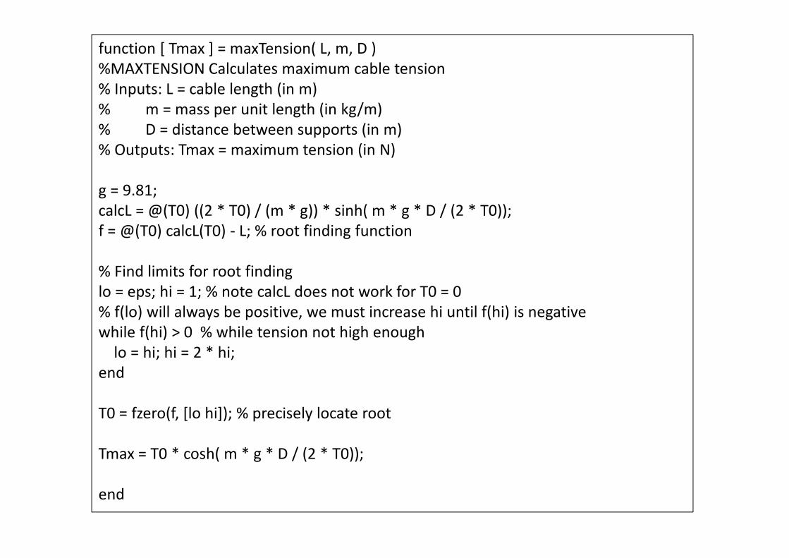
function [ Tmax ] = maxTension( L, m, D )

%MAXTENSION Calculates maximum cable tension

% Inputs: L = cable length (in m)

% m = mass per unit length (in kg/m)

% D = distance between supports (in m)

% Outputs: Tmax = maximum tension (in N)

g = 9.81;

calcL = @(T0) ((2 * T0) / (m * g)) * sinh( m * g * D / (2 * T0));

f = @(T0) calcL(T0) - L; % root finding function

% Find limits for root finding

lo = eps; hi = 1; % note calcL does not work for T0 = 0

% f(lo) will always be positive, we must increase hi until f(hi) is negative

while f(hi) > 0 % while tension not high enough

lo = hi; hi = 2 * hi;

end

T0 = fzero(f, [lo hi]); % precisely locate root

Tmax = T0 * cosh( m * g * D / (2 * T0));

end

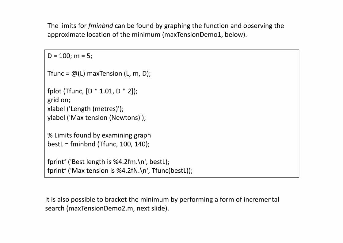
D = 100; m = 5;

Tfunc = @(L) maxTension (L, m, D);

fplot (Tfunc, [D * 1.01, D * 2]);

grid on;

xlabel ('Length (metres)');

ylabel ('Max tension (Newtons)');

% Limits found by examining graph

bestL = fminbnd (Tfunc, 100, 140);

fprintf ('Best length is %4.2fm.\n', bestL);

fprintf ('Max tension is %4.2fN.\n', Tfunc(bestL));

The limits for fminbnd can be found by graphing the function and observing the

approximate location of the minimum (maxTensionDemo1, below).

It is also possible to bracket the minimum by performing a form of incremental

search (maxTensionDemo2.m, next slide).

D = input ('Enter D: '); m = input ('Enter m: ');

Tfunc = @(L) maxTension (L, m, D);

fplot (Tfunc, [D * 1.01, D * 2]);

grid on;

xlabel ('Length (metres)');

ylabel ('Max tension (Newtons)');

% bracket the minimum

L1 = D * 1.001; L2 = D * 1.002; T2 = Tfunc(L2); % assume tension falling

while 1

L3 = L2 + 1; T3 = Tfunc(L3);

if T3 > T2 % tension has started going up

break;

end;

L1 = L2; L2 = L3; T2 = T3;

end

bestL = fminbnd (Tfunc, L1, L3);

fprintf ('Best length is %4.2fm.\n', bestL);

fprintf ('Max tension is %4.2fN.\n', Tfunc(bestL));

Key points to note:

The “function” in a root finding or optimization problem need not correspond to a

simple mathematical expression.

Instead it can be any process which converts an input value into an output value.

A function can involve hundreds of lines of code and complex procedures.

Function evaluation can take a significant amount of time (hours, in extreme

cases).

It is desirable to keep the number of function evaluations required by a procedure

to a minimum.

Save function results that will be required later instead of re-evaluating the

function. Example: Compare the bisection search in these notes (bisect.m, one

function evaluation per iteration) with the one on page 127 of Chapra 2nd ed or

p139 of Chapra 3rd ed (which evaluates the function twice per iteration).

When function evaluations take a lot of time faster search methods become

relatively more attractive.