08-01 estimating dea confidence intervals for canadian ... 2001, and since then at least 15 more...
TRANSCRIPT

Estimating DEA Confidence Intervals for Canadian Urban Paratransit Agencies Using Panel Data Analysis Darold T. Barnum*, University of Illinois at Chicago John M. Gleason, Creighton University Brendon Hemily, Brendon Hemily and Associates * Darold T. Barnum is the corresponding author Great Cities Institute College of Urban Planning and Public Affairs University of Illinois at Chicago Great Cities Institute Publication Number: GCP-08-01 A Great Cities Institute Working Paper January 2008

The Great Cities Institute The Great Cities Institute is an interdisciplinary, applied urban research unit within the College of Urban Planning and Public Affairs at the University of Illinois at Chicago (UIC). Its mission is to create, disseminate, and apply interdisciplinary knowledge on urban areas. Faculty from UIC and elsewhere work collaboratively on urban issues through interdisciplinary research, outreach and education projects.
About the Author Darold T. Barnum, University of Illinois at Chicago ([email protected]) is Professor of
Management and Professor of Information & Decision Sciences at the University of Illinois at Chicago. He formerly was an Associate Director at the Indiana University Institute for Urban Transportation, where he participated in the training of transit managers from across the nation. His research focuses on performance measurement.
John M. Gleason, Creighton University ([email protected]) is a Professor in the
Department of Information Systems and Technology within in the College of Business Administration at Creighton University in Omaha.
Brendon Hemily, Brendon Hemily and Associates ([email protected]) is a Principal for Brendon Hemily and Associates located in Toronto, Canada. Great Cities Institute Publication Number: GCP-08-01
The views expressed in this report represent those of the author(s) and not necessarily those of the Great Cities Institute or the University of Illinois at Chicago. GCI working papers may represent research in progress. Inclusion here does not preclude final preparation for publication elsewhere. Great Cities Institute (MC 107) College of Urban Planning and Public Affairs University of Illinois at Chicago 412 S. Peoria Street, Suite 400 Chicago IL 60607-7067 Phone: 312-996-8700 Fax: 312-996-8933 http://www.uic.edu/cuppa/gci
UIC Great Cities Institute

UIC Great Cities Institute
Estimating DEA Confidence Intervals for Canadian Urban Paratransit Agencies Using Panel Data Analysis Abstract This paper illustrates three concepts new to the Data Envelopment Analysis (DEA) literature, and applies them to data from Canadian urban paratransit agencies. First, it predicts valid confidence intervals and trends for each agency’s true efficiency. Second, it uses Panel Data Analysis methodology, a set of statistical procedures that are more likely to produce valid estimates than those commonly used in DEA studies. Third, it uses a new method of identifying and adjusting for environmental effects that has more power than conventional procedures.
UIC Great Cities Institute
INTRODUCTION
Data Envelopment Analysis (DEA) has been increasingly utilized to compare urban transit
agency performance. De Borger, Kerstens and Alvaro (2002) identify 15 articles published
before 2001, and since then at least 15 more have been published or are in press (Boilé 2001,
Nolan et al. 2001, Novaes 2001, Odeck and Alkadi 2001, Pina and Torres 2001, De Borger et
al. 2002, Nolan et al. 2002, Karlaftis 2003, Boame 2004, Karlaftis 2004, Brons et al. 2005,
Odeck 2006, Sheth et al. 2006, Graham 2006, Barnum et al. 2006).
The reason for DEA’s popularity is easy to understand. In one of the earlier DEA studies of
urban transit, Chu, Fielding and Lamar (1992, p. 224) argue that “performance analysis needs
to progress from multiple measures and partial comparison to more robust indicators of
performance . . . so that the achievements of one agency can be examined in reference to peer
group agencies.” More recently, Brons et al (2005, pp. 1-2) add “it is of great interest to
investigate whether urban transit operators work in a technically efficient way (i.e. reach
economic targets such as cost minimization or output maximization conditional on output or
input constraints). Solid technical efficiency (TE) measurement can provide a significant
contribution.” DEA provides a single comparative measure of technical efficiency in analyses
involving multiple inputs and multiple outputs, so it is uniquely equipped to fulfill the needed role.
One of DEA’s major shortcomings is that it reports only a point estimate of the technical
efficiency of a Decision Making Unit (DMU), with no indication of the interval within which the
DMU’s true technical efficiency is likely to occur (Boame 2004). A DEA score is composed of
both true efficiency and statistical noise, but the entire score is treated as true efficiency.
Without an estimate of the size and characteristics of the disturbance term, it is impossible to
determine with statistical significance whether a given DMU is efficient (Grosskopf 1996).
Bootstrapping of cross-sectional data has been used to estimate the confidence interval
within which a true production frontier occurs, with the results used to estimate the range within
1
UIC Great Cities Institute
which the DEA score of a fixed input-output set occurs (Xue and Harker 1999, Simar and
Wilson 2004, Boame 2004). However, the reported confidence interval for the target DMU’s
efficiency is solely the result of variation of the production frontier, because the statistical noise
in the target DMU’s data is not taken into consideration. Boame (2004, p. 404) states it more
elegantly: “the bootstrap efficiency estimate for the ith firm is evaluated as the efficiency of the
original input xi relative to the bootstrapped isoquant of the input set.” Thus, these
bootstrapping procedures account for stochastic variations in the production frontier (the
isoquant), but do not address stochastic variations in the inputs and outputs of the target DMU.
So, they alone cannot estimate the range within which a target DMU’s true efficiency occurs.
In order to estimate the interval within which a given DMU’s true DEA efficiency occurs, it is
necessary to utilize multiple observations of each DMU’s efficiency scores, which, of course, is
true for any stochastic variable. Cross sectional data have only one observation for each DMU,
so they cannot be used to estimate these confidence intervals. If panel (longitudinal) data are
available, but they are analyzed by cross-sectional methods or by pooling, then they also do not
provide the multiple observations needed. To date, all urban transit DEA studies that have
panel data have used cross-sectional methods or pooling (Chang and Kao 1992, Nolan 1996,
Button and Costa 1999, Nolan et al. 2001, Nolan et al. 2002, Karlaftis 2003, Karlaftis 2004), and
we are aware of only one DEA study with panel data that does not do so (Steinmann and
Zweifel 2003).
In this paper, therefore, we use Panel Data Analysis (PDA), a unique set of statistical
methods that are much more informative than the statistical techniques used in current DEA
research (Wooldridge 2002, Hsiao 2003, Frees 2004, Baltagi 2005, Baum 2006). By
simultaneously estimating the cross-sectional and longitudinal aspects of panel data, PDA
2

UIC Great Cities Institute
makes it possible to develop valid confidence intervals for individual DMUs, and also it improves
the power, precision and validity of other statistical estimates.
Another important issue for DEA is the need to identify exogenous influences in order to
explain variations in DEA scores caused by factors external to the DMUs, both for policy
purposes and in order to correctly evaluate the endogenous efficiency of individual DMUs.
Two-stage methods are the most popular procedures for identifying environmental influences.
With the conventional two-stage method, a DEA is first conducted using only traditional
(endogenous) inputs and outputs. Then, the first-stage DEA scores are regressed on the
environmental/contextual (exogenous) variables of interest. The regression outcomes are
used to identify exogenous inputs that influence the first-stage DEA scores to a statistically
significant degree, and to adjust DEA scores to account for these influences. Statistical
significance tests usually are based on asymptotic theory, although some prefer
bootstrapping (Kerstens 1996, Pina and Torres 2001, Ray 2004, Cooper et al. 2004, Boame
2004, Coelli et al. 2005, Simar and Wilson 2007).
While it has been long suspected (Grosskopf 1996, Coelli et al. 2005), it recently has been
demonstrated that the conventional two-stage method exhibits substantial bias, low precision,
and low power (Barnum and Gleason 2007). These results were based on asymptotic
methods. However, bootstrapping also has been shown to have low power in detecting true
relationships (Zelenyuk 2005).
A reverse two-stage procedure, that yields estimates without the bias, precision and power
problems that compromise the validity of the conventional method’s estimates, has been
demonstrated with simulated data (Barnum and Gleason 2007). In essence, this procedure
reverses the conventional method’s steps. In the first stage, the endogenous (traditional)
inputs of interest are regressed on the exogenous (environmental) factors expected to
influence them. The resulting estimates are used to adjust the endogenous inputs to remove
3
UIC Great Cities Institute
the marginal influence of exogenous factors. In the second stage, the outputs and adjusted
inputs are analyzed by DEA, with the resulting scores being independent of exogenous
effects. (The same procedure could be applied to outputs, if they were influenced by
exogenous factors.) Herein, we apply the reverse two stage method to real-world empirical
data, using PDA instead of the conventional statistical methods.
With this paper, therefore, we illustrate three new techniques for DEA research. First, we
provide a valid method for estimating confidence intervals for individual DMUs. Second, we
apply Panel Data Analysis to all statistical procedures. Third, we illustrate an improved two-
stage method for adjusting for environmental influences.
We apply these techniques to DEA efficiency measurement of urban paratransit
operations, in itself an important topic that has not been much addressed previously. In the
only paper of which we are aware, Viton (1997) included both conventional bus and demand-
responsive urban transit in his DEA, but did not analyze them separately. As noted in a
current Transit Cooperative Research Program project (2006), “Demand-response
transportation (DRT) systems are under increasing pressure to improve performance because
of increased demand for service and financial constraints. . . To identify opportunities for
improvement, DRT systems need better . . . methods to measure and assess performance.”
For this study, we use Canadian urban paratransit data because it is more detailed than U.S.
data, and also because it will be only the second DEA study using Canadian transit data
(Boame 2004).
THE DATA SET, OUR ASSUMPTIONS, AND PREVIEW OF THE PAPER
Data are from 28 Canadian urban paratransit agencies for 1996-2004. They include all
agencies that reported the data needed for this analysis (Canadian Urban Transit
Association, 1996-2004).
4

UIC Great Cities Institute
As is typical with traditional DEA, we do not suggest that these 28 DMUs are a random
sample that is representative of all possible paratransit agencies at all possible times. The 28
DMUs represent the population and time period of interest, and those that are reported to be
efficient define the true production frontier. That is, we adopt the concept that a DMU’s
relative efficiency is determined solely by comparisons with the other DMUs in the analysis
(Charnes et al. 1978, Cooper et al. 2004). In contrast to traditional DEA, we address the fact
that any DEA score is composed of both the true level of technical efficiency and a random
error component.
Below, the inputs and outputs are identified and justified. The first stage Panel Data
Analysis is used to adjust the endogenous inputs to remove the effects of exogenous
(environmental) influences. The second stage DEA model is presented, followed by the
statistical model used in the second stage Panel Data Analysis. The results of diagnostic
tests on the second-stage statistical error terms are presented. Finally, for each DMU, the
predicted values, confidence intervals and trends that resulted from the procedure are
examined, followed by the results of the conventional two-stage method and our conclusions.
DEA INPUTS AND OUTPUTS
Canadian urban paratransit agencies are the DMUs, with each using two inputs to produce
four outputs. Inputs are (1) annual operating expenses of paratransit service dedicated to
disabled individuals, and (2) annual operating expenses attributable to disabled riders of non-
dedicated paratransit service. Outputs are (1) annual number of disabled passenger trips on
paratransit service dedicated to disabled individuals, (2) annual number of disabled
passenger trips on non-dedicated paratransit service, (3) annual operating revenue from
dedicated paratransit service, and (4) annual operating revenue attributable to disabled riders
of non-dedicated paratransit service. This particular set of inputs and outputs, and
organizational subunits, is based on those considered key by the industry and reflected in the
5

UIC Great Cities Institute
set of published performance indicators that are used to compare agencies (Canadian Urban
Transit Association, 1996-2004).
Two key outputs of Canadian urban paratransit agencies are disabled passenger trips and
operating revenue (mostly fares). Fare levels vary significantly among systems and years;
consequently, passenger trip and revenue values measure two unique outputs. Agencies
have different mixes of these two outputs, because increases in one lead to decreases in the
other when fares are changed, holding inputs constant (Litman 2004). In setting fare levels, it
would never be a behavioral objective of these agencies to minimize costs or to maximize
either revenues or profits. Generally, fares are set at levels that local decision makers
consider “fair,” and may be based on factors such as local farebox recovery ratio objectives
and local mass transit fares. This will result in a variety of revenue-rider ratios, none being
universally superior because of the absence of a common behavioral objective.
Both outputs are produced by two distinct organizational subunits: a subunit serving only
disabled users (dedicated service), and a subunit serving both disabled and non-disabled
users (non-dedicated service). Dedicated service is provided by vehicles exclusively
dedicated to the transport of persons with disabilities, which may be operated by the agency
itself or subcontracted. Non-dedicated service is provided by vehicles that serve both
disabled and non-disabled customers, often taxicabs subcontracted by the paratransit agency
to transport its disabled clients.
Operating expenses are used as a proxy for physical inputs. It is more typical in transit
DEA studies to use physical inputs, most often labor, fuel and vehicles (De Borger et al.
2002). We have not done so for the following reasons. DEA assumes that there is
substitutability among inputs, with diminishing marginal rates of substitution (Petersen 1990).
For paratransit, this would mean that, to produce a fixed level of output, a DMU could
6
UIC Great Cities Institute
substitute labor for vehicles, or substitute vehicles for fuel. In truth, there is very little
substitutability in this industry; inputs have to be used in a virtually fixed ratio, with any excess
being wasted. Disaggregating non-substitutable inputs would usually result in some truly
inefficient units being reported as efficient. As is well known, increasing the number of inputs
and outputs results in higher efficiency scores, whether or not they are justified. Also, the
number of DMUs reporting slacks normally will increase, making the radial technical efficiency
scores less meaningful. Finally, because of the random error component in all variables, the
larger the number of inputs and outputs, the more likely that a DMU’s efficiency score will be
increased by random chance. Therefore, more valid technical efficiency scores will be
reported if we aggregate the types of input resources that are not substitutes, weighting them
by their prices, which is a conventional economic solution (Färe et al. 1994).
For this analysis, all inputs and outputs are limited to those related to disabled passengers.
However, because there are two quite unique methods of providing transportation (dedicated
or non-dedicated service), and two different organizational subunits with independent
production processes, inputs and outputs from each are entered as separate variables. This
disaggregation is necessary to avoid bias in the reported DEA scores. Recent research
demonstrates that, for inputs and outputs that are allocable and substitutable for each other,
as ours are, disaggregated data must be used to avoid bias in efficiency scores (Tauer 2001,
Färe and Zelenyuk 2002, Färe et al. 2004, Färe and Grosskopf 2004, Barnum and Gleason
2005a, Barnum and Gleason 2005b, Barnum and Gleason 2006a, Barnum and Gleason
2006b).
THE FIRST STAGE STATISTICAL MODEL: ADJUSTING FOR EXOGENOUS FACTORS
In this study, the exogenous variables of interest are those that influence the level of input
resources needed to produce a given amount of output. In paratransit, production and
consumption are identical because trips are demand-based (unlike conventional transit where
7

UIC Great Cities Institute
more output is produced than consumed). Therefore, when analyzing paratransit efficiency in
converting inputs into outputs, we do not have to deal with produced vs. consumed outputs,
and the potential for erroneous performance indicators (Gleason and Barnum 1978, Gleason
and Barnum 1982).
Exogenous Influences on Urban Paratransit Efficiency
A number of exogenous variables that might influence Canadian urban paratransit input
levels were considered. These included (1) annual snowfall, (2) whether the dedicated
service was operated by the agency itself, contracted to a non-profit agency, or contracted to
a for-profit management services company, (3) input resource price differences, and (4)
average length of a passenger trip.
We expected areas with higher annual snowfalls to have higher expenses per trip,
because most expenses are time-based and such areas could be expected to have slower
travel speeds. Furthermore, there might be increased time involved in getting disabled
passengers into and out of vehicles. Annual snowfall data for each of the nine years were
collected for each of the 28 communities involved.
Dedicated service is provided by one of three options: the paratransit agency itself,
another non-profit agency under contract with the paratransit agency, or a for-profit
management services company under contract with the paratransit agency. We did not make
predictions on the direction of influence.
A very high percentage of paratransit operating expenses is for employee compensation.
Although Canadian data are not available, for U.S. paratransit in 2004, 82 percent of
operating expenses was for employee compensation, followed by 6 percent for fuel, 6 percent
for insurance, 5 percent for materials and supplies, and 1 percent for utilities (Danchenko
2006). And, average compensation varies substantially among the 28 Canadian agencies,
8
UIC Great Cities Institute
with the 2004 operator top base wage rate ranging from $14.82 to $24.32 per hour. Typically,
most other wage rates in the dedicated service subunit are indexed on the operator top base
wage rate, which also can serve as a proxy for wage rate variation in the non-dedicated
subunit because it reflects local labor market conditions. It is likely that other operating
expenses also will show somewhat similar variation due to local cost differences. Because
employee compensation is mainly a reflection of the local labor market, and therefore largely
beyond the control of the local management, its level is one of the exogenous variables for
which we must adjust. We expect higher base rates to result in higher expenses per trip.
Because of exogenous factors such as geography and population density, trips will be
longer in some areas than in others, and average speed will differ. The net effect of these
local environmental factors can be summarized by the average number of vehicle hours per
passenger. We would expect DMUs providing longer trips to have higher expenses per trip.
Statistical Models and Outcomes
Variables that have no statistically significant influence are annual snowfall, and whether
the dedicated service was provided by the paratransit agency, another non-profit agency, or a
for-profit management services company. We don’t present that model herein. The variables
that do have a statistically significant influence are operator top base wage rate and vehicle
hours per passenger:
1 2 3log( ) log( ) log( ) log( )jt j jt jt jt jtDOE DedPass Wage VHPP uα β β β= + + + + (1)
1 2 3log( ) log( ) log( ) log( )jt j jt jt jt jtNOE NDedPass Wage VHPP uα β β β= + + + + (2)
The subscript j = 1,…,28 represents the DMU involved and the subscript t = 1,…,9
represents the year. DOE is operating expenses for dedicated service, and NOE is operating
expenses for non-dedicated service. DedPass is the number of passengers carried by the
9

UIC Great Cities Institute
dedicated subunit and NDedPass is the number of disabled passengers carried by the non-
dedicated subunit. Wage is the operator top base rate in the dedicated subunit, and VHPP is
the number of vehicle hours per passenger in the dedicated subunit. Because we have Wage
and VHPP data only for the dedicated subunit, in the non-dedicated subunit they serve as
proxies for the relative price of resources and the relative length of time traveled for the
community involved. Finally, jα is the time-constant effect that reflects the unique
characteristics of DMU j, and is the error term for DMU j in year t. jtu
In order to correctly specify the models, it is necessary to include the number of
passengers carried as an independent variable. Clearly, the main driver of operating
expenses is passenger trips. If they were not included, some of their effect might be
attributed to either wages or vehicle hours per passenger, and a host of other problems might
result from an incorrectly specified model.
To estimate the parameters of these models we use PDA, treating the individual effect
( jα ) as a fixed effect, with robust variance-covariance estimation in order to adjust for
arbitrary serial correlation and heteroskedasticity. We used a fixed effect model in order to
allow arbitrary correlation between the three observed explanatory variables and the
individual effect jα . The residuals of the two equations were not correlated with each other
[ 2R = 0.007, F(1, 175) = 0.13, P(F(1,175) > 0.13 = 0.7208] , so we did not estimate the two
equations as a set using Zellner’s Seemingly Unrelated Regressions (SUR) model
(Wooldridge 2002). All statistical analysis was conducted with Stata 9.2 (StataCorp 2007).
The results are presented in Tables 1 and 2.
10

UIC Great Cities Institute
We use the expected values of the regression coefficients for wages and vehicle hours per
passenger to remove the effects of these variables from the value of operating expenses for
both subunits, namely
(3) Adjusted log( ) log( ) 1.4991log( ) 0.3050log( ). jt jt jt jtDOE DOE Wage VHPP= − −
(4) Adjusted log( ) log( ) 1.2656log( ) 0.5081log( ). jt jt jt jtNOE NOE Wage VHPP= − −
Note that these adjusted values retain any inefficiency contained in each DMU’s individual
intercept ( jtujα ), as well as retaining its residual error ( ). Only the expected effects of the
exogenous variables are removed. The two adjusted input values and four original outputs
are used in DEA.
THE SECOND STAGE DEA MODEL
For each of the nine years of data, DEA scores are computed using linear program (5) that
is output oriented and reflects the constant returns to scale of this industry. The DEAs were
conducted with Scheel’s EMS software (2000). For each of the j DMUs (j = 1,…,28), there
are data on the n = 2 inputs x 11( ,..., )jnx x , and on the m = 4 outputs y . The DEA
score θ identifies the technical super-efficiency of the target DMU k (Andersen and Petersen
1993).
11( ,..., )jmy y
maxθλ
28
1jm j km
jy yλ θ
=≥∑subject
to 1,2,3,4m =
28
1jn j kn
jx xλ
=≤∑ 1,2n =
0kλ =
11

UIC Great Cities Institute
0jλ ≥ 1,2,..., 28;j j k= ≠ (5)
The technical efficiency rather than the technical super-efficiency indicator would have
been appropriate if our interest had focused on identifying the production frontier, those
DMUs defining it, and the distance of inefficient DMUs from it. In that model, inefficient DMUs
are compared to their efficient peers, but efficient DMUs are compared only to themselves.
We are interested in always comparing the performance of each DMU to its efficient peers,
whether or not it contributes to defining the production frontier. Super-efficiency scores
provide the necessary comparison, because they always compare each DMU to its efficient
peers regardless of its own efficiency level.
A second reason for using super-efficiency scores is to avoid a censored dependent
variable in second-stage regressions (Coelli et al. 2005). Conventional technical efficiency
scores yield a censored variable, because an efficient DMU’s score of 1 will remain
unchanged even if it were to become more productive by increasing outputs or decreasing
inputs. Super-efficiency scores are an observable proxy for latent variable values underlying
conventional efficiency scores, and they remove the need to estimate latent values using
Tobit, sample-selected, or truncated regression (Breen 1996).
THE SECOND STAGE STATISTICAL MODEL
We use Panel Data Analysis with the fixed effects model because we wish to estimate the
efficiencies of the specific 28 DMUs in the study, and the inferences are restricted to
developing confidence intervals for the efficiency of each of these specific DMUs when
compared to the remaining DMUs in the set (Baltagi 2005). The statistical model is
( 1)j jt j j jtw t uθ α β= + − + (6) 1,...,28; 1,...,9j t= =
12

UIC Great Cities Institute
jtθ is the super-efficiency score of DMU j in year t, jα jβ is the individual effect of DMU j,
is the annual change in the individual effect jα of DMU j, and is the random error in the
super-efficiency score (
jtu
jtθ ) of DMU j in year t. Many DMUs showed linear trends in
efficiency over the nine year period, so equation 6 includes a factor (t-1) that adjusts
efficiency for the year involved, which permits a heterogeneous trend in each DMU’s
efficiency over the nine-year period. No exogenous variables are included in the model
because their effects already have been removed via the first stage statistical model.
Not surprisingly, the unweighted scores resulted in heteroskedastic error terms among the
DMUs. Because we develop confidence intervals for each DMU’s true efficiency, we want the
estimates to be statistically efficient as well as consistent. Therefore, each DMU’s scores
were weighted by , an index based on the standard deviation of its errors when the
unweighted scores were used.
jw
After weighting the dependent variable, the error terms were homoskedastic; the Breusch-
Pagan/Cook-Weisberg test for heteroskedasticity found no statistically significant differences
at the
2χ 2χ 2χ0.05 level among the DMUs [ (27) = 0.03, P( > 0.03) = 1.0000], over time [ (1) =
0.01, P( 2χ 2χ > 0.01) = 0.9383], or by expected value of the response variable [ (1) = 0.02,
P( 2χ > 0.02) = 0.8965].
ERROR TERM DIAGNOSTICS
For confidence intervals from a correctly specified regression model, residuals usually are
assumed to be independent and identically distributed (i.i.d.), and Normally distributed. When
the response variable is a DEA score, these characteristics cannot be taken for granted. The
main reason for this is because each DMU’s score is influenced by the performance of other
13
UIC Great Cities Institute
DMUs. If the same DMUs consistently influence each other, it may cause correlations among
their error terms. Such contemporaneous correlation would invalidate the requirement for
independent residuals (Xue and Harker 1999, Simar and Wilson 2007).
Although contemporaneous correlation does not bias the expected value of estimated
efficiency levels, variance estimates can be more precise if the correlation is taken into
account. That is, if the residuals are contemporaneously correlated to a statistically
significant degree, one could use the estimates in a Generalized Least Squares model to
decrease standard errors.
Tests for contemporaneous correlation cannot be conducted if the data are cross-
sectional, or if cross-sectional methods are used on panel data. Using PDA, however, such
tests are available. If the number of DMUs exceeds the number of time periods, as is true for
our data, then tests for cross-sectional independence of residuals include Freedman’s AVER
and Frees’ 2AVER evaluated with his Q-distribution (Frees 1995, Frees 2004), Pesaran’s
cross-sectional dependence test (Baum 2006, p. 222), and the pairwise correlation of
residuals.
CD
AVER AVER = 8.438, P(The results are CD = 0.073, P( CD > |0.073| ) = 0.9422; and > 8.438)
=0.9998. None of the pair-wise correlations were statistically significant at the 0.05 level,
using either Bonferroni-adjusted significance tests or Sidak-adjusted significance tests.
However, 2AVER = 1.392, which is statistically significant at the 0.05 level.
Because only three of the four tests reported no statistically significant contemporaneous
correlation, the evidence was not unanimous. The conservative decision would be to assume
that there is no cross-correlation. This decision permits the use of more robust statistical
14
UIC Great Cities Institute
models, which report the same mean values but wider variances. Therefore we do not
correct for possible cross-correlation.
There are other conditions violating i.i.d and Normal distribution assumptions that cannot
be identified with conventional methods, but can be tested for (and corrected) with PDA.
These include heteroskedasticity across DMUs, the Normal distribution of residuals, and
serial correlation.
As discussed earlier, the Breusch-Pagan/Cook-Weisberg test for heteroskedasticity found
no statistically significant differences among the DMUs. The Shapiro-Wilk W test did not
reject the hypothesis of Normality [z =0.599, P(z > 0.599) = 0.275]. To test for first-order
serial correlation, we regressed each residual on the prior year’s residual using all 80 of the
available observations. Because the fixed effect model demeans the data, if the true error
terms are uncorrelated then the estimated errors will have a correlation coefficient of -1/(T-1),
with T equal to the number of observations for each DMU (Wooldridge 2002). Because T = 5,
ˆ 0.3349ρ = −0.25ρ = − if there is no serial correlation. Here, , with a standard error of 0.1070,
which is not different from -0.25 to a statistically significant degree.
In sum, the null hypotheses that the residuals are i.i.d. and Normally distributed cannot be
rejected. This demonstrates that violations of the standard parametric assumptions by DEA
residuals are not inevitable. It may be worthwhile to recall that any disturbance term
encapsulates complicated, unidentified interactions with the variables in question, so it is
never truly random. But, a residual can be treated as random if it meets appropriate statistical
tests for randomness (Frees 2004). So, we make the standard asymptotic assumptions in
developing confidence intervals from equation 6.
RESULTS FOR THE REVERSE TWO-STAGE PROCEDURE
The regression based on equation 6 had an R-square of 0.9837 [F(55, 196) = 215.10,
P(F(55,196) >215.10) < 0.00005]. Because the equation permits heterogeneous trends in 15

UIC Great Cities Institute
each DMU’s efficiency, we tested to assure that trends indeed were present. Using the Chow
test to compare the full model with a reduced model in which the trend variables are removed,
the difference was statistically significant at the 0.05 level [F(28, 196) = 5.90, P(F(28, 196) >
5.90) < 0.00005]. Therefore, for at least some of the DMUs, there are statistically significant
trends in their efficiency levels over the nine year period.
The DEA model is output oriented, so higher scores mean lower efficiency. The
confidence intervals are based on the standard error of prediction of the true mean value, at
the 0.90 level of confidence. These scores have been “unweighted” in Table 3, so they are
normal super-efficiency measures.
As shown in Table 3, the 2004 point estimates of the mean efficiency for 16 DMUs showed
them to be inefficient, but 6 of these were not inefficient to a statistically significant degree. Of
the 12 DMUs with efficient mean point estimates, 8 were not efficient to a statistically
significant degree. Thus, whether 14 of the 28 systems were or were not efficient in 2004
cannot be determined with statistical confidence.
Therefore, the point estimates of the expected efficiency for a given year should not be
used to positively identify their levels of efficiency, because the range within which their true
efficiency could occur is often going to overlap the inefficient and efficient ranges. Indeed,
because the actual DEA scores for 2004 have a much wider variation than the estimated
mean scores, attempting to determine a DMU’s true efficiency from those single data points
would be even more unwise.
ˆ 0jβ <Whether each DMU’s trend in efficiency is statistically significant also is of interest.
indicates efficiency is increasing, and indicates efficiency is decreasing. For the
DMUs, 18 report increasing efficiency over the nine years involved, of which 12 show
ˆ 0jβ >
16

UIC Great Cities Institute
statistically significant improvements. On the other hand, 10 report decreasing efficiency over
the nine year period, of which 5 are worse to a statistically significant degree.
RESULTS FOR THE CONVENTIONAL TWO-STAGE PROCEDURE
It is of interest to compare the results of our reverse two-stage procedure used above with
the results of the conventional two-stage procedure. Under the conventional two-stage
procedure, first DEA scores are calculated from the unadjusted, endogenous inputs and
outputs, and second the unadjusted scores are regressed on the exogenous variables. We
did so, using linear program 5 for the DEA and statistical model 7 for the regression. Model 7
is identical to model 6, except that the two exogenous factors are included as independent
variables. Those applying the conventional procedure make the standard i.i.d. and Normality
assumptions, but cannot verify them because of their use of cross-sectional methods, so we
don’t verify those assumptions here.
1 2( ) ( ) ( 1)jt jtjt j jVHPP Wage t u jtλ λ α β= + + + − + 1,..., 28; 1,...9j tθ = = (7)
The data cannot validly be pooled, because the nine error terms of each DMU (one for
each of the nine years) are not independent when the data are pooled; indeed, when the
residuals from the pooled data are regressed on their own residuals lagged by one year, the
regression coefficient is 0.82, t = 22.4 (P>|t| < 0.00005), and R2 = 0.69. Further, comparing
the full model in equation 7 with a reduced model that includes only the VHPP and Wage
variables, the full model explains 90 percent of the variance in efficiency scores, as compared
to only 26 percent for the reduced model; these values differ to a statistically significant
degree [F (57,201) = 50.11, P (F(57,201) >50.11 <0.00005)], so the reduced model is miss-
specified. Any pooling of this data, or the use of any one-year cross section, would yield
invalid estimates and confidence intervals.
17

UIC Great Cities Institute
For the regression using equation 7, the regression coefficient of VHPP is -0.236, which is
in the right direction, but its t-ratio is only 0.91, not significant at the 0.37 level. The
regression coefficient for Wage is -0.236, which is in the right direction, but it has a t-ratio of
only -0.68 so it is not significant at the 0.50 level. In short, neither exogenous variable is
reported to affect the DEA score to a statistically significant degree. This is not surprising
because both are significantly correlated with endogenous inputs, as shown in Tables 1 and
2; Barnum and Gleason (2007) have shown that the power of the conventional two-stage
procedure to detect the effects of exogenous factors rapidly decreases as correlation
between the exogenous variables and endogenous inputs increases.
CONCLUSIONS
As exhibited in this paper, Panel Data Analysis provides a methodology for estimating valid
confidence intervals for the DEA efficiency of individual DMUs. It addresses noise in the data
of the target DMU and the production frontier, and it makes it possible to test residuals before
accepting (or rejecting) the standard asymptotic assumptions. By exploiting the advantages
of simultaneous estimation of the cross-sectional and longitudinal aspects of panel data, it
increases the validity of all parameter estimations, and permits identification of statistically
significant trends.
Further, the paper demonstrates a new method of identifying and adjusting for the effects
of environmental variables on efficiency, herein called the reverse two-stage method. The
reverse two-stage method is shown to have more power to detect environmental effects than
the conventional two-stage procedure, at least in situations where the endogenous inputs and
exogenous influences are correlated, and it avoids some of the other well-known statistical
shortcomings of the conventional method.
18
UIC Great Cities Institute
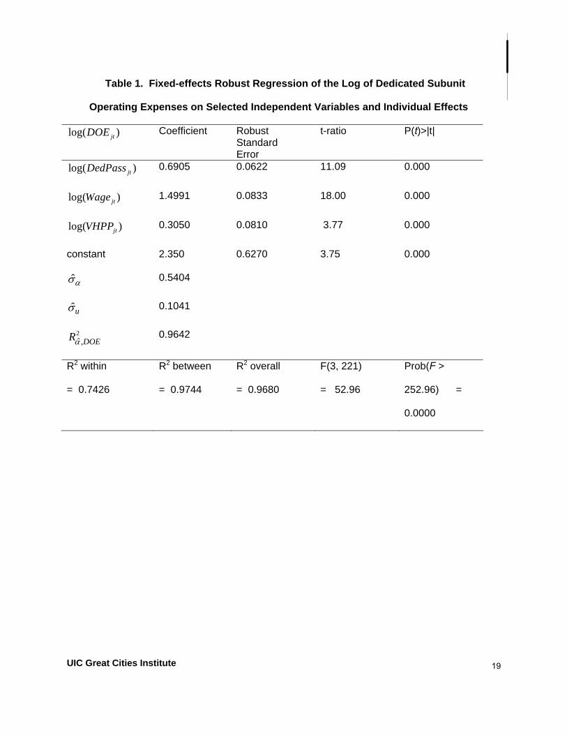
Table 1. Fixed-effects Robust Regression of the Log of Dedicated Subunit
Operating Expenses on Selected Independent Variables and Individual Effects
Coefficient Robust Standard Error
t-ratio P(t)>|t| log( )jtDOE
0.6905 0.0622 11.09 0.000 log( )jtDedPass
1.4991 0.0833 18.00 0.000 log( )jtWage
0.3050 0.0810 3.77 0.000 log( )jtVHPP
constant 2.350 0.6270 3.75 0.000
0.5404 ˆασ
0.1041 ˆuσ
0.9642 2ˆ ,DOERα
R2 within
= 0.7426
R2 between R2 overall F(3, 221) Prob(F >
252.96) =
0.0000
= 0.9744 = 0.9680 = 52.96
19

UIC Great Cities Institute
Table 2. Fixed-effects Robust Regression of the Log of Non-Dedicated Subunit
Operating Expenses on Selected Independent Variables and Individual Effects
Coefficient Robust Standard Error
t-ratio P(t)>|t| log( )jtNOE
0.9220 0.0598 15.41 0.000 log( )jtNDedPass
1.2656 0.2457 5.15 0.000 log( )jtWage
0.5081 0.1668 3.05 0.003 log( )jtVHPP
constant 0.0016 0.6929 0.00 0.998
0.3286 ˆασ
0.2414 ˆuσ
0.6496 2ˆ ,NOERα
R2 within
= 0.7657
R2 between R2 overall F(3,153) Prob(F >
146.89) =
0.0000
= 0.9711 = 0.9615 = 146.89
20

UIC Great Cities Institute
Table 3. 2004 Super-efficiency Scores, 28 Canadian Urban Paratransit Properties
2004 Super-efficiency Score, Output Oriented (0.90 Confidence Interval)
Mean Annual Change
Lower limit jDMU
9( )jE θ Upper limit Conclusion ˆ( )jβ
1 1.003 0.818 1.188 Inefficient 0.017 2 0.925 0.760 1.090 Efficient -0.008 3 1.291 1.186 1.396 Inefficient* -0.036* 4 0.735 0.610 0.861 Efficient* 0.062* 5 1.036 0.951 1.121 Inefficient -0.007 6 0.955 0.742 1.167 Efficient -0.06* 7 0.992 0.753 1.232 Efficient -0.083* 8 0.867 0.727 1.007 Efficient -0.034* 9 1.282 1.189 1.374 Inefficient* 0.001
10 1.182 1.010 1.355 Inefficient* -0.035 11 1.043 0.838 1.249 Inefficient -0.05* 12 0.750 0.503 0.998 Efficient* -0.048 13 1.530 1.435 1.624 Inefficient* -0.012 14 1.282 1.212 1.352 Inefficient* 0.029* 15 0.868 0.772 0.965 Efficient* 0.002 16 0.853 0.810 0.895 Efficient* -0.009 17 1.089 0.954 1.223 Inefficient -0.066* 18 1.108 0.972 1.245 Inefficient 0.019 19 0.968 0.907 1.029 Efficient 0.002 20 0.989 0.867 1.111 Efficient -0.064* 21 2.090 1.949 2.232 Inefficient* 0.041* 22 0.874 0.702 1.047 Efficient -0.104* 23 1.235 1.145 1.324 Inefficient* -0.03* 24 1.448 1.406 1.490 Inefficient* -0.019* 25 1.086 1.018 1.154 Inefficient* -0.017* 26 0.852 0.666 1.038 Efficient 0.044* 27 1.030 0.940 1.120 Inefficient -0.042* 28 1.288 1.134 1.442 Inefficient* 0.036*
* Statistically significant at the 0.10 two-tailed level.
ˆ 0jβ <9( )jE 9( )jE1θ ≤ 1θ >Note: is efficient, is inefficient, indicates the DMU is
becoming more efficient, and indicates the DMU is becoming less efficient. ˆ 0jβ >
21
UIC Great Cities Institute
References
Andersen, P. and Petersen, N. C. (1993). "A procedure for ranking efficient units in data
envelopment analysis." Management Science, 39(10), 1261-1265.
Baltagi, B. H. (2005). Econometric analysis of panel data, John Wiley & Sons, Ltd, West
Sussex, England.
Barnum, D. T. and Gleason, J. M. (2005a). "Technical efficiency bias caused by intra-input
aggregation in data envelopment analysis." Applied Economics Letters, 12(13), 785-788.
Barnum, D. T. and Gleason, J. M. (2005b) Technical efficiency bias in data envelopment
analysis caused by intra-output aggregation. Forthcoming in Applied Economics Letters.
Barnum, D. T. and Gleason, J. M. (2006a). "Biases in technical efficiency scores caused by
intra-input aggregation: Mathematical analysis and a DEA application using simulated
data." Applied Economics, 38 1593-1603.
Barnum, D. T. and Gleason, J. M. (2006b). "Measuring efficiency in allocating inputs among
outputs with DEA." Applied Economics Letters, 13(6), 333-336.
Barnum, D. T. and Gleason, J. M. (2007) Bias and precision in the DEA two-stage method.
Forthcoming in Applied Economics.
Barnum, D. T., McNeil, S., and Hart, J. (2006). "Comparing the efficiency of public
transportation subunits using data envelopment analysis. Forthcoming in the Journal of
Public Transportation.
Baum, C. F. (2006). An introduction to modern econometrics using Stata, Stata Press,
College Station, Texas.
Boame, A. K. (2004). "The technical efficiency of Canadian urban transit systems."
Transportation Research Part E-Logistics and Transportation Review, 40(5), 401-416.
22
UIC Great Cities Institute
Boilé, M. P. (2001). "Estimating technical and scale inefficiencies of public transit systems."
Journal of Transportation Engineering, 127(3), 187-194.
Breen, R. (1996). Regression models: Censored, sample-selected, or truncated data, Sage
Publications, Thousand Oaks, Ca.
Brons, M., Nijkamp, P., Pels, E. and Rietveld, P. (2005). "Efficiency of urban public transit: A
meta analysis." Transportation, 32(1), 1-21.
Button, K. and Costa, A. (1999). "Economic efficiency gains from urban public transport
regulatory reform: Two case studies of changes in Europe." The Annals of Regional
Science, 33(4), 425-438.
Canadian Urban Transit Association (1996-2004 ) Specialized transit services fact books:
1996-2004 operating data. Toronto, Canada, Canadian Urban Transit Association.
Chang, K. P. and Kao, P. H. (1992). "The relative efficiency of public versus private municipal
bus firms: An application of data envelopment analysis." Journal of Productivity Analysis,
3 67-84.
Charnes, A., Cooper, W. W. and Rhodes, E. (1978). "Measuring the efficiency of decision
making units." European Journal of Operational Research, 2(6), 429-444.
Chu, X., Fielding, G. J. and Lamar, B. W. (1992). "Measuring transit performance using data
envelopment analysis." Transportation Research Part A: Policy and Practice, 26(3), 223-
230.
Coelli, T. J., Rao, D. S. P., O'Donnell, C. J. and Battese, G. E. (2005). An introduction to
efficiency and productivity analysis, Springer, New York, NY.
Cooper, W. W., Seiford, L. M. and Zhu, J. (2004) Data envelopment analysis: History, models
and interpretations. Handbook on Data Envelopment Analysis eds W. W. Cooper, L. M.
Seiford and J. Zhu, pp. 1-40. Kluwer Academic Publishers, Boston.
23

UIC Great Cities Institute
Danchenko, D. (2006). "Public Transportation Fact Book,"
<http://www.apta.com/research/stats/factbook/documents/2006factbook.pdf> (May 24,
2006).
De Borger, B., Kerstens, K. and Costa, A. (2002). "Public transit performance: What does
one learn from frontier studies?" Transport Reviews, 22(1), 1-38.
Färe, R., Grosskopf, S. and Zelenyuk, V. (2004). "Aggregation bias and its bounds in
measuring technical efficiency." Applied Economics Letters, 11(10), 657-660.
Färe, R. and Grosskopf, S. (2004). New directions: Efficiency and productivity, Kluwer
Academic Publishers, Boston.
Färe, R., Grosskopf, S. and Lovell, C. A. K. (1994). Production frontiers, Cambridge Univ.
Press, Cambridge, Eng.
Färe, R. and Zelenyuk, V. (2002). "Input aggregation and technical efficiency." Applied
Economics Letters, 9(10), 635-636.
Frees, E. W. (1995). "Assessing cross-sectional correlation in panel data." Journal of
Econometrics, 69(2), 393-414.
Frees, E. W. (2004). Longitudinal and panel data: Analysis and applications in the social
sciences, Cambridge University Press, Cambridge, U.K.
Gleason, J. M. and Barnum, D. T. (1978). "Caveats Concerning Efficiency/Effectiveness
Measures of Mass Transit Performance." Management Science, 24(16), 1777-1778.
Gleason, J. M. and Barnum, D. T. (1982). "Toward valid measures of public sector
productivity: Performance indicators in urban transit." Management Science, 28(4), 379-
386.
24

UIC Great Cities Institute
Graham, D. J. (2006). "Productivity and efficiency in urban railways: Parametric and non-
parametric estimates." Transportation Research Part E: Logistics and Transportation
Review, In Press, Corrected Proof
Grosskopf, S. (1996). "Statistical inference and nonparametric efficiency: A selective survey."
Journal of Productivity Analysis, 7(2-3), 161-176.
Hsiao, C. (2003). Analysis of panel data, Cambridge University Press, Cambridge.
Karlaftis, M. G. (2003). "Investigating transit production and performance: A programming
approach." Transportation Research Part A-Policy and Practice, 37(3), 225-240.
Karlaftis, M. G. (2004). "A DEA approach for evaluating the efficiency and effectiveness of
urban transit systems." European Journal of Operational Research, 152(2), 354-364.
Kerstens, K. (1996). "Technical efficiency measurement and explanation of French urban
transit companies." Transportation Research Part A: Policy and Practice, 30(6), 431-452.
Litman, T. (2004). "Transit price elasticities and cross-elasticities." Journal of Public
Transportation, 7(2), 37-58.
Nolan, J. F., Ritchie, P. C. and Rowcroft, J. E. (2002). "Identifying and measuring public
policy goals: ISTEA and the US bus transit industry." Journal of Economic Behavior &
Organization, 48(3), 291-304.
Nolan, J. F., Ritchie, P. C. and Rowcroft, J. R. (2001). "Measuring efficiency in the public
sector using nonparametric frontier estimators: A study of transit agencies in the USA."
Applied Economics, 33(7), 913-922.
Nolan, J. F. (1996). "Determinants of productive efficiency in urban transit." Logistics and
Transportation Review, 32(3), 319-342.
Novaes, A. G. N. (2001). "Rapid transit efficiency analysis with the assurance-region DEA
method." Pesquisa Operacional, 21(2), 179-197.
25

UIC Great Cities Institute
Odeck, J. and Alkadi, A. (2001). "Evaluating efficiency in the Norwegian bus industry using
data envelopment analysis." Transportation, 28(3), 211-232.
Odeck, J. (2006). "Congestion, ownership, region of operation, and scale: Their impact on
bus operator performance in Norway." Socio-Economic Planning Sciences, 40(1), 52-69.
Petersen, N. C. (1990). "Data envelopment analysis on a relaxed set of assumptions."
Management Science, 36(3), 305-314.
Pina, V. and Torres, L. (2001). "Analysis of the efficiency of local government services
delivery: An application to urban public transport." Transportation Research Part A-Policy
and Practice, 35(10), 929-944.
Ray, S. C. (2004). Data envelopment analysis: Theory and techniques for economics and
operations research, Cambridge University Press, Cambridge, UK.
Scheel, H. (2000). "EMS: Efficiency Measurement System," <http://www.wiso.uni-
dortmund.de/lsfg/or/scheel/ems/ > (Dec. 17, 2000).
Sheth, C., Triantis, K. and Teodorovic, D. (2006). "Performance evaluation of bus routes: A
provider and passenger perspective." Transportation Research Part E: Logistics and
Transportation Review, In Press, Corrected Proof
Simar, L. and Wilson, P. W. (2004) Performance of the bootstrap for DEA estimators and
iterating the principle. Handbook on Data Envelopment Analysis eds W. W. Cooper, L. M.
Seiford and J. Zhu, pp. 265-298. Kluwer, Boston.
Simar, L. and Wilson, P. W. (2007). "Estimation and inference in two-stage, semi-parametric
models of production processes." Journal of Econometrics, 136(1), 31-64.
StataCorp, Stata Statistical Software. Release 9.2, 2007.
Steinmann, L. and Zweifel, P. (2003). "On the (in)efficiency of Swiss hospitals." Applied
Economics, 35(3), 361-370.
26

UIC Great Cities Institute
Tauer, L. W. (2001). "Input aggregation and computed technical efficiency." Applied
Economics Letters, 8(5), 295-297.
Transit Cooperative Research Program. (2006). "Guidebook for Measuring, Assessing, and
Improving Performance of Demand-Response Transportation," <
http://www4.trb.org/trb/crp.nsf/All+Projects/TCRP+B-31>
Viton, P. A. (1997). "Technical efficiency in multi-mode bus transit: A production frontier
analysis." Transportation Research Part B: Methodological, 31(1), 23-39.
Wooldridge, J. M. (2002). Econometric analysis of cross section and panel data, MIT Press,
Cambridge, MA.
Xue, M. and Harker, P. T. (1999). "Overcoming the inherent dependency of DEA efficiency
scores: A bootstrap approach, 99-17, Financial Institutions Center, Wharton School, Univ.
of Pennsylvania, Philadelphia, PA," <http://fic.wharton.upenn.edu/fic/papers/99/9917.pdf>
Zelenyuk, V. (2005). "Power of significance test of dummies in Simar-Wilson two-stage
efficiency analysis model, DP0522, Institut de Statistique, Université Catholique de
Louvain, Belgium," <http://www.stat.ucl.ac.be/ISpub/ISdp.html#2005>
27