06887356

632 IEEE TRANSACTIONS ON AUTOMATIC CONTROL, VOL. 60, NO. 3, MARCH 2015

Discrete-Time Solutions to the Continuous-TimeDifferential Lyapunov Equation With

Applications to Kalman FilteringPatrik Axelsson and Fredrik Gustafsson, Fellow, IEEE

Abstract—Prediction and filtering of continuous-time stochasticprocesses often require a solver of a continuous-time differentialLyapunov equation (CDLE), for example the time update in theKalman filter. Even though this can be recast into an ordinarydifferential equation (ODE), where standard solvers can be ap-plied, the dominating approach in Kalman filter applications is todiscretize the system and then apply the discrete-time differenceLyapunov equation (DDLE). To avoid problems with stabilityand poor accuracy, oversampling is often used. This contribu-tion analyzes over-sampling strategies, and proposes a novel low-complexity analytical solution that does not involve oversampling.The results are illustrated on Kalman filtering problems in bothlinear and nonlinear systems.

Index Terms—Continuous time systems, discrete time systems,Kalman filters, sampling methods.

I. INTRODUCTION

NUMERICAL solvers for ordinary differential equations(ODE) is a well studied area [1]. The related area of

Kalman filtering (state prediction and state estimation) incontinuous-time models was also well studied during the firsttwo decades of the Kalman filter, see for instance [2], whilethe more recent literature such as the standard reference [3]focuses on discrete time filtering only. A specific example, withmany applications in practice, is Kalman filtering based ona continuous-time state space model with discrete-time mea-surements, known as continuous-discrete filtering. The Kalmanfilter (KF) here involves a time update that integrates the first-and second-order moments from one sample time to the nextone. The second-order moment is a covariance matrix, andit governs a continuous-time differential Lyapunov equation(CDLE). The problem can easily be recast into a vectorizedODE problem and standard solvers can be applied. For linearODE’s, the time update of the linear KF can thus be solvedanalytically, and for nonlinear ODE’s, the time update of theextended KF has a natural approximation in continuous-time.One problem is the large dimension of the resulting ODE. An-other possible explanation why the continuous-time update isnot used is the common use of discrete-time models in Kalmanfilter applications, so practitioners often tend to discretize the

Manuscript received December 17, 2012; revised February 10, 2014;accepted August 4, 2014. Date of publication August 28, 2014; date of currentversion February 19, 2015. This work was supported by the Vinnova ExcellenceCenter LINK-SIC. Recommended by Associate Editor Z. Wang.

The authors are with the Division of Automatic Control, Department ofElectrical Engineering, Linköping University, SE-581 83 Linköping, Sweden(e-mail: [email protected]; e-mail: [email protected]).

Color versions of one or more of the figures in this paper are available onlineat http://ieeexplore.ieee.org.

Digital Object Identifier 10.1109/TAC.2014.2353112

state space model first to fit the discrete-time Kalman filtertime update. Despite a closed form solution exists, this involvesapproximations that lead to well known problems with accuracyand stability. The ad-hoc remedy is to oversample the system,so a large number of small time updates are taken between thesampling times of the observations.

In literature, different methods are proposed to solve thecontinuous-discrete nonlinear filtering problem using extendedKalman filters (EKF). A common way is to use a first orsecond-order Taylor approximation as well as a Runge–Kuttamethod in order to integrate the first-order moments, see, e.g.,[4]–[6]. They all have in common that the CDLE is replacedby the discrete-time difference Lyapunov equation (DDLE),used in discrete-time Kalman filters. A more realistic way isto solve the CDLE as is presented in [7], [8], where the first-and second-order moments are integrated numerically. A com-parison between different solutions is presented in [9], wherethe method proposed by the authors discretizes the stochasticdifferential equation (SDE) using a Runge–Kutta solver. Theother methods in [9] have been proposed in the literature before,e.g., [4] and [8]. Related work using different approximationsto continuous integration problems in nonlinear filtering alsoappears in [10] and [11] for unscented Kalman filters and [12]for cubature Kalman filters.

This contribution takes a new look at this fundamentalproblem. First, we review different approaches for solving theCDLE in a coherent mathematical framework. Second, weanalyze in detail the stability conditions for oversampling, andbased on this we can explain why even simple linear modelsneed a large rate of oversampling. Third, we make a newstraightforward derivation of a low-complexity algorithm tocompute the solution with arbitrary accuracy. Numerical stabil-ity and computational complexity is analyzed for the differentapproaches. It turns out that the low-complexity algorithm hasbetter numerical properties compared to the other methods, andat the same time a computational complexity in the same order.Fourth, the methods are extended to nonlinear system where theextended Kalman filter (EKF) is used. We illustrate the resultson both a simple second-order linear spring-damper system,and a nonlinear spring-damper system relevant for mechanicalsystems, in particular robotics.

II. MATHEMATICAL FRAMEWORK AND BACKGROUND

A. Linear Stochastic Differential Equations

Consider the linear stochastic differential equation (SDE)

dx(t) = Ax(t)dt+Gdβ(t) (1)

0018-9286 © 2014 IEEE. Personal use is permitted, but republication/redistribution requires IEEE permission.See http://www.ieee.org/publications_standards/publications/rights/index.html for more information.

AXELSSON AND GUSTAFSSON: DISCRETE-TIME SOLUTIONS TO THE CDLE 633

for t ≥ 0, where x(t) ∈ Rnx is the state vector and β(t) ∈ R

nβ

is a vector of Wiener processes with E[dβ(t)dβ(t)T] = Qdt.The matrices A ∈ R

nx×nx and G ∈ Rnx×nβ are here assumed

to be constants, but they can also be time varying. It is alsopossible to include a control signal u(t) in (1) giving a bit morecomplicated expression for the first-order moment.

Given an initial state x(0) with covariance P (0), we want tosolve the SDE to get x(t) and P (t) at an arbitrary time instance.By multiplying both sides with the integrating factor e−As andintegrating over the time interval gives

x(t) = eAtx(0) +

t∫0

eA(t−s)Gdβ(s)

︸︷︷︸vd(t)

. (2)

The goal is to get a discrete-time update of the mean and covari-ance, from x(kh) and P (kh) to x((k + 1)h) and P ((k + 1)h),respectively. The time interval h may correspond to one sampleinterval, or be a fraction of it in the case of oversampling. Thelatter case will be discussed in detail later on. For simplicity,the time interval [kh, (k + 1)h] will be denoted as [0, t] below.

The discrete-time equivalent noise vd(t) has covariancegiven by

Qd(t)=

t∫0

eA(t−s)GQGTeAT(t−s)ds=

t∫0

eAτGQGTeATτdτ.

(3)

We immediately get an expression for the first- and second-order moments of the SDE solution over one time interval as

x(t) = eAtx(0) (4a)

P (t) = eAtP (0)eATt +Qd(t). (4b)

From (2) and (3), we can also recover the continuous-timeupdate formulas

˙x(t) =Ax(t) (5a)

P (t) =AP (t) + P (t)AT +GQGT (5b)

by, a bit informally, taking the expectation of (2) and thendividing both sides with t and letting t → 0. A formal proofof (5) can be based on Itô’s lemma, see [2]. Equation (5a) isan ordinary ODE and (5b) is the continuous-time differentialLyapunov equation (CDLE).

Thus, there are two conceptually different alternatives.Either, solve the integral (3) defining Qd(t) and use (4), or solvethe ODE and CDLE in (5). These two well-known alternativesare outlined below.

B. Matrix Fraction Decomposition

There are two ways to compute the integral (3) described inliterature. Both are based on computing the matrix exponentialof the matrix

H =

(A GQGT

0 −AT

). (6)

The result is a block matrix in the form

eHt =

(M1(t) M2(t)

0 M3(t)

)(7)

where the structure implies that M1(t) = eAt and M3(t) =

e−ATt. As shown in [13], the solution to (3) can be computed as

Qd(t) = M2(t)M1(t)T. (8)

This is immediately verified by taking the time derivative of thedefinition (3) and the matrix exponential (7), and verifying thatthe involved Taylor expansions are equal.

Another alternative known as matrix fraction decomposition,which solves a matrix valued ODE, given in [14] and [15], is tocompute P (t) directly. Using the initial conditions (P (0) I)T

for the ODE gives

P (t) = (M1(t)P (0) +M2(t))︸︷︷︸Δ=C(t)

M3(t)−1. (9)

The two alternatives in (8) and (9) are apparently algebraicallythe same.

There are also other alternatives described in literature. First,the integral in (3) can of course be solved with numerical meth-ods such as the trapezoidal method or the rectangle method.In [16] the integral is solved analytically in the case that Ais diagonalizable. However, not all matrices are diagonaliz-able, and even in such cases, this method is not numericallystable [17].

C. Vectorization Method

The ODEs for the first- and second-order moments in (5)can be solved using a method based on vectorization. Thevectorization approach for matrix equations is well known andespecially for the CDLE, see, e.g., [18] and [19]. The methoduses the fact that (5) can be converted to one single ODE byintroducing an extended state vector

z(t) =

(zx(t)zP (t)

)=

(x(t)

vechP (t)

)(10)

z(t) =

(A 00 AP

)z(t) +

(0

vechGQGT

)= Azz(t) +Bz

(11)

where AP = D†(I ⊗A+A⊗ I)D. Here, vech denotes thehalf-vectorization operator, ⊗ is the Kronecker product and Dis a duplication matrix, see Appendix A for details.

The solution of the ODE (11) is given by [20]

z(t) = eAztz(0) +

t∫0

eAz(t−τ)dτBz. (12)

One potentially prohibitive drawback with the solution in (12)is its computational complexity, in particular for the matrix ex-ponential. The dimension of the extended state z is nz = nx +nx(nx + 1)/2, giving a computational complexity of O(n6

x).Section IV presents a way to rewrite (12) to give a complexityof O(n3

x) instead of O(n6x).


D. Discrete-Time Recursion of the CDLE

The solution in (4b) using (8), the matrix fraction decompo-sition in (9), and the ODE (12) evaluated at the discrete-timeinstances t = kh and t = (k + 1)h give the following recursiveupdate formulas:

P ((k + 1)h) = eAhP (kh)eATh +M2(h)M1(h)

T (13)P ((k + 1)h) = (M1(h)P (kh) +M2(h))M3(h)

−1 (14)

z ((k + 1)h) = eAzhz(kh) +

h∫0

eAzτdτBz (15)

which can be used in the Kalman filter time update.

E. Matrix Exponential

Section II-A–C show that the matrix exponential function is aworking horse to solve the linear SDE. At this stage, numericalroutines for the matrix exponential are important to understand.One key approach is based on the following identity and Taylorexpansion, [21]

eAh =(e

Ahm

)m≈(I +

(Ah

m

)+ · · ·+ 1

p!

(Ah

m

)p)mΔ= ep,m(Ah).

(16)

In fact, the Taylor expansion is a special case of a more generalPadé approximation of eAh/m [21], but this does not affect thediscussion here.

The eigenvalues of Ah/m are the eigenvalues of A scaledwith h/m, and thus they can be arbitrarily small if m is chosenlarge enough for any given h. Further, the pth-order Taylorexpansion converges faster for smaller eigenvalues of Ah/m.Finally, the power function Mm is efficiently implemented bysquaring the matrix M in total log2(m) times, assuming that mis chosen to be a power of 2. We will denote this approximationwith ep,m(Ah).

A good approximation ep,m(Ah) is characterized by thefollowing properties:

• Stability. If A has all its eigenvalues in the left half plane,then ep,m(Ah) should have all its eigenvalues inside theunit circle.

• Accuracy. If p and m are chosen large enough, the error‖eAh − ep,m(Ah)‖ should be small.

Since the Taylor expansion converges, we have trivially that

limp→∞

ep,m(Ah) =(e

Ahm

)m= eAh. (17a)

From the property limx→∞(1 + a/x)x = ea, we also have

limm→∞

ep,m(Ah) = eAh. (17b)

Finally, from [17] we have that

∥∥eAh − ep,m(Ah)∥∥ ≤ ‖A‖p+1hp+1

mp(p+ 1)!e‖A‖h. (17c)

However, for any finite p and m > 1, then all terms in thebinomial expansion of ep,m(Ah) are different from the Taylor

expansion of eAh, except for the first two terms which arealways I +Ah.

The complexity of the approximation ep,m(Ah), where A ∈R

nx×nx , is in the order of (log2(m) + p)n3x, where pn3

x multi-plications are required to compute Ap and log2(m)n3

x multipli-cations are needed for squaring the Taylor expansion log2(m)times.

Standard numerical integration routines can be recast intothis framework as well. For instance, a standard tuning of thefourth-order Runge–Kutta method for a linear ODE results ine4,1(Ah).

F. Solution Using Approximate Discretization

We have now outlined three methods to compute the exacttime update in the discrete-time Kalman filter. These should beequivalent up to numerical issues, and will be treated as oneapproach in the sequel.

Another common approach in practice, in particular inKalman filter applications, is to assume that the noise is piece-wise constant giving the discrete-time system

x(k + 1) =Fhx(k) +Ghvh(k) (18a)cov (vh(k)) =Qh (18b)

where Fh = ep,m(Ah), Gh =∫ h

0 eAtdtG, and Qh = hQ. Thediscrete-time Kalman filter update equations

x(k + 1) =Fhx(k) (19a)P (k + 1) =FhP (k)FT

h +GhQhGTh (19b)

are then used, where (19a) is a difference equation and (19b) isthe discrete-time difference Lyapunov equation (DDLE). Theupdate (19) are exact for the discrete-time model (18). However,there are several approximations involved in the discretizationstep:

• First, Fh = ep,m(Ah) is an approximation of the exactsolution given by Fh = eAh. It is quite common in prac-tice to use Euler sampling defined by Fh = I +Ah =e1,1(Ah).

• Even without process noise, the update formula for P in(19b) is not equivalent to (5b).

• The discrete-time noise vh(t) is an aggregation of thetotal effect of the Wiener process dβ(t) during the interval[t, t+ h], as given in (3). The conceptual drawback is thatthe Wiener process dβ(t) is not aware of the sampling timechosen by the user.

One common remedy is to introduce oversampling. This meansthat (19) is iterated m times using the sampling time h/m.When oversampling is used, the covariance matrix for thediscrete-time noise vh(k) should be scaled as Qh = hQ/m. Inthis way, the problems listed above will asymptotically vanishas m increases. However, as we will demonstrate, quite large anm can be needed even for some quite simple systems.

G. Summary of Contributions

• Section III gives explicit conditions for an upper boundof the sample time h such that a stable continuous-timemodel remains stable after discretization. The analysistreats stability of both x and P , for the case of Euler


TABLE ISUMMARY OF APPROXIMATIONS ep,m(Ah) OF eAh. THE STABILITY

REGION (h < hmax) IS PARAMETRIZED IN λi WHICH ARE THE

EIGENVALUES TO A. IN THE CASE OF RUNGE–KUTTA,ONLY REAL EIGENVALUES ARE CONSIDERED

sampling e1,m(A), for the solution of the SDE given bythe ODE (11). Results for p > 1 are also briefly discussed.See Table I for a summary when the vectorized solutionis used.

• Section IV presents a reformulation of the solution to theODE (11), where the computational complexity has beendecreased from (log2(m) + p)(n2

x/2)3 to (log2(m) +

p+ 43)n3x.

• Section V shows how the computational complexity andthe numerical properties differs between the differentmethods.

• Section VI presents a second-order spring-damper exam-ple to demonstrate the advantages using a continuous-timeupdate.

• Section VII discusses implications for nonlinear systems,and investigates a nonlinear system inspired by applica-tions in robotics.

III. STABILITY ANALYSIS

It is known that the CDLE in (5b) has a unique positive solu-tion P (t) if A is Hurwitz,1 GQGT 0, the pair (A,

√GQGT)

is controllable, and P (0) � 0 [19]. We want to show that astable continuous-time system results in a stable discrete-timerecursion. We therefore assume that the continuous-time ODEdescribing the state vector x(t) is stable; hence, the eigenvaluesλi, i = 1, . . . , n to A are assumed to be in the left half plane,i.e., �e{λi} < 0, i = 1, . . . , nx. It will also be assumed that theremaining requirements are fulfilled.

For the methods described in Section II-B we have that Hin (6) has the eigenvalues ±λi, i = 1, . . . , nx, where λi are theeigenvalues of A. This follows from the structure of H . Hence,the matrix exponential eHt will have terms that tend to infinityand zero with the same exponential rate when t increases.However, the case t = h is of most interest, where h is finite.Note that a small/large sample time depends strongly on thesystem dynamics. Even if the matrix eHt is ill-conditioned,the product (8) and the ratio (9) can be limited under theassumptions above, for not too large values of t. Note that thesolution in (9) is, as a matter of fact, based on the solution ofan unstable ODE, see [14], [15], but the ratio C(t)M3(t)

−1

can still be bounded. Both of these methods can have numericalproblems which will be discussed in Section V-B.

1All eigenvalues are in the left half plane.

A. Stability for the Vectorization Method Using Euler Sampling

The stability analysis in this section is standard and a similaranalysis has been performed in [22]. The difference is thatthe analysis in [22] investigates which discretization methodsthat are stable for sufficiently small sample times. The analysishere is about to find an upper bound of the sample timesuch that a stable continuous-time model remains stable afterdiscretization.

The recursive solution (15) is stable for all h according toLemma 9 in Appendix B, if the matrix exponential can becalculated exactly. Stability issues arise when eAzh has to beapproximated by ep,m(Azh). In this section, we derive an upperbound on h that gives a stable solution for e1,m(Azh), i.e.,Euler sampling. The Taylor expansion and in particular Eulersampling is chosen due to its simplicity, the same approach isapplicable to the Padé approximation as well. Higher ordersof approximations using the Taylor expansion will be treatedbriefly at the end of this section.

From Section II-C we have that the matrix Az is diagonal,which means that calculation of the matrix exponential eAzh

can be separated into eAh and eAPh. From [23] it is knownthat the eigenvalues of AP are given by λi + λj , 1 ≤ i ≤ j ≤nx; hence, the ODE describing the CDLE is stable if A isHurwitz. In order to keep the discrete-time system stable, theeigenvalues of both e1,m(Ah) and e1,m(APh) need to be insidethe unit circle. In Theorem 1, an explicit upper bound on thesample time h is given that makes the recursive solution to thecontinuous-time SDE stable.

Theorem 1: The recursive solution to the SDE (1), in theform of (15), where the matrix exponential eAzh is approxi-mated by e1,m(Azh), is stable if

h < min

{−2mRe{λi + λj}

|λi + λj |2, 1 ≤ i ≤ j ≤ nx

}(20)

where λi, i = 1, . . . , n, are the eigenvalues to A.Corollary 2: The bound in Theorem1 becomes

h < −2m

λi, λi ∈ R (21)

for real eigenvalues.Proof: Start with the ODE describing the state vector

x(t). The eigenvalues to e1,m(Ah) = (I +Ah/m)m are, ac-cording to Lemma 8 in Appendix B, given by (1 + λih/m)m.The eigenvalues are inside the unit circle if |(1 + λih/m)m| <1, where∣∣∣∣(1 +

λih

m

)m∣∣∣∣ =(

1

m

√m2 + 2aihm+ (a2i + b2i )h

2

)m

.

(22)

In (22), the parametrization λi = ai + ibi has been used. Solv-ing |(1 + λih/m)m| < 1 for h and using the fact |λi|2 = a2i +b2i give

h < −2mai|λi|2

. (23)

Similar calculations for the ODE describing vechP (t) give

h < −2m(ai + aj)

|λi + λj |2, 1 ≤ i ≤ j ≤ nx. (24)


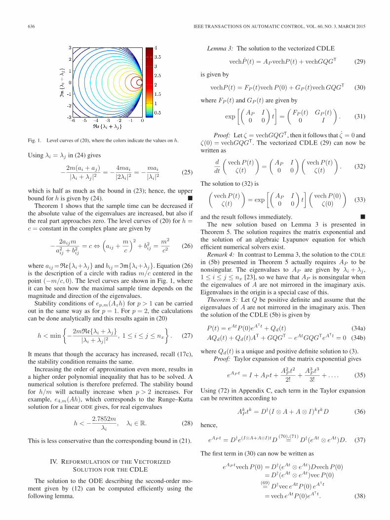
Fig. 1. Level curves of (20), where the colors indicate the values on h.

Using λi = λj in (24) gives

−2m(ai + aj)

|λi + λj |2= − 4mai

|2λi|2= −mai

|λi|2(25)

which is half as much as the bound in (23); hence, the upperbound for h is given by (24). �

Theorem 1 shows that the sample time can be decreased ifthe absolute value of the eigenvalues are increased, but also ifthe real part approaches zero. The level curves of (20) for h =c = constant in the complex plane are given by

− 2aijm

a2ij + b2ij= c ⇔

(aij +

m

c

)2+ b2ij =

m2

c2(26)

where aij=Re{λi+λj} and bij=Im{λi+λj}. Equation (26)is the description of a circle with radius m/c centered in thepoint (−m/c, 0). The level curves are shown in Fig. 1, whereit can be seen how the maximal sample time depends on themagnitude and direction of the eigenvalues.

Stability conditions of ep,m(Azh) for p > 1 can be carriedout in the same way as for p = 1. For p = 2, the calculationscan be done analytically and this results again in (20)

h < min

{−2mRe{λi + λj}

|λi + λj |2, 1 ≤ i ≤ j ≤ nx

}. (27)

It means that though the accuracy has increased, recall (17c),the stability condition remains the same.

Increasing the order of approximation even more, results ina higher order polynomial inequality that has to be solved. Anumerical solution is therefore preferred. The stability boundfor h/m will actually increase when p > 2 increases. Forexample, e4,m(Ah), which corresponds to the Runge–Kuttasolution for a linear ODE gives, for real eigenvalues

h < −2.7852m

λi, λi ∈ R. (28)

This is less conservative than the corresponding bound in (21).

IV. REFORMULATION OF THE VECTORIZED

SOLUTION FOR THE CDLE

The solution to the ODE describing the second-order mo-ment given by (12) can be computed efficiently using thefollowing lemma.

Lemma 3: The solution to the vectorized CDLE

vechP (t) = APvechP (t) + vechGQGT (29)

is given by

vechP (t) = FP (t)vechP (0) +GP (t)vechGQGT (30)

where FP (t) and GP (t) are given by

exp

[(AP I0 0

)t

]=

(FP (t) GP (t)0 I

). (31)

Proof: Let ζ = vechGQGT, then it follows that ζ = 0 andζ(0) = vechGQGT. The vectorized CDLE (29) can now bewritten as

d

dt

(vechP (t)

ζ(t)

)=

(AP I0 0

)(vechP (t)

ζ(t)

). (32)

The solution to (32) is(vechP (t)

ζ(t)

)= exp

[(AP I0 0

)t

](vechP (0)

ζ(0)

)(33)

and the result follows immediately. �The new solution based on Lemma 3 is presented in

Theorem 5. The solution requires the matrix exponential andthe solution of an algebraic Lyapunov equation for whichefficient numerical solvers exist.

Remark 4: In contrast to Lemma 3, the solution to the CDLE

in (5b) presented in Theorem 5 actually requires AP to benonsingular. The eigenvalues to AP are given by λi + λj ,1 ≤ i ≤ j ≤ nx [23], so we have that AP is nonsingular whenthe eigenvalues of A are not mirrored in the imaginary axis.Eigenvalues in the origin is a special case of this.

Theorem 5: Let Q be positive definite and assume that theeigenvalues of A are not mirrored in the imaginary axis. Thenthe solution of the CDLE (5b) is given by

P (t) = eAtP (0)eATt +Qd(t) (34a)

AQd(t) +Qd(t)AT +GQGT − eAtGQGTeA

Tt = 0 (34b)

where Qd(t) is a unique and positive definite solution to (3).Proof: Taylor expansion of the matrix exponential gives

eAP t = I +AP t+A2

P t2

2!+

A3P t

3

3!+ . . . . (35)

Using (72) in Appendix C, each term in the Taylor expansioncan be rewritten according to

AkP t

k = D†(I ⊗A+A⊗ I)ktkD (36)

hence,

eAP t = D†e(I⊗A+A⊗I)tD(70),(71)

= D†(eAt ⊗ eAt)D. (37)

The first term in (30) can now be written as

eAP tvechP (0) =D†(eAt ⊗ eAt)DvechP (0)

=D†(eAt ⊗ eAt)vecP (0)(69)= D†vec eAtP (0) eA

Tt

=vech eAtP (0)eATt. (38)


Similar calculations give

eAP tvechGQGT = D†veceAtGQGTeATt Δ

= vechQ(t). (39)

It is easily verified using the Taylor expansion of (31) thatGP (t) = A−1

P (eAP t − I). The last term in (30) can thereforebe rewritten according to

A−1P

(eAP t − I

)vechGQGT =A−1

P vech(Q(t)−GQGT

)Δ=vechQd(t) (40)

where it is assumed that AP is invertible. Equation (40) canbe seen as the solution of the linear system of equationsAPvechQd(t) = vech(Q(t)−GQGT). Using the derivationin (64) in Appendix A backwards gives that Qd(t) is thesolution to the algebraic Lyapunov equation

AQd(t) +Qd(t)AT +GQGT − Q(t) = 0. (41)

Combining (38) and (40) gives that (30) can be written as

P (t) = eAtP (0)eATt +Qd(t) (42)

where Qd(t) is the solution to (41).It is easily verified that Qd(t) in (3) satisfies (41) and it is

well known that the Lyapunov equation has a unique solutioniff the eigenvalues of A are not mirrored in the imaginary axis[19]. Moreover, the assumption that Q is positive definite givesfrom (3) that Qd(t) is positive definite; hence, the solution to(41) is unique and guaranteed to be positive definite under theassumptions on A. �

If Lemma 3 is used directly, a matrix exponential of a matrixof dimension nx(nx + 1)× nx(nx + 1) is required. Now, onlythe Lyapunov equation (34b) has to be solved, where thedimensions of the matrices are nx × nx. The computationalcomplexity for solving the Lyapunov equation is 35n3

x [17].The total computational complexity for computing the solutionof (5b) using Theorem 5 is (log2(m) + p+ 43)n3

x, where(log2(m) + p)n3

x comes from the matrix exponential, and 43n3x

comes from solving the Lyapunov equation (35n3x) and taking

four matrix products giving 2n3x each time.

The algebraic Lyapunov function (34b) has a unique solutiononly if the eigenvalues of A are not mirrored in the imaginaryaxis [19], as a result of the assumption that AP is nonsingular,and this is the main drawback with using Theorem 5 rather thanusing Lemma 3. In the case of integrators, the method presentedin [24] can be used. To be able to calculate Qd(t), the methodtransforms the system such that the Lyapunov equation (34b) isused for the subspace without the integrators, and the integralin (3) is used for the subspace containing the integrators.

Discrete-time Recursion: The recursive solution to the dif-ferential equations in (5) describing the first and second-ordermoments of the SDE (1) can now be written as

x ((k + 1)h) = eAhx(kh) (43a)

P ((k + 1)h) = eAhP (kh)eATh +Qd(h) (43b)

AQd(h) +Qd(h)AT +GQGT − eAhGQGTeA

Th = 0. (43c)

Equations (43b) and (43c) are derived using t = kh and t =(k + 1)h in (34).

TABLE IISIX VARIANTS TO CALCULATE P (t). THE LAST COLUMN SHOWS

THE COMPUTATIONAL COMPLEXITY p IN O(npx) WHICH

IS DESCRIBED IN DETAIL IN SECTION V-A

The method presented in Theorem 5 is derived straightfor-wardly from Lemma 3. A similar solution that also solves analgebraic Lyapunov function is presented in [18]. The main dif-ference is that Theorem 5 gives a value of the covariance matrixQd(t) for the discrete-time noise explicitly, as opposed to thesolution in [18]. Moreover, the algebraic Lyapunov function in[18] is independent of time, which is not the case here sinceeAtGQGTeA

Tt changes with time. This is not an issue for therecursive time update due to the fact that eAhGQGTeA

Th isonly dependent on h; hence, the algebraic Lyapunov equation(43c) has to be solved only once.

V. COMPARISON OF SOLUTIONS FOR THE CDLE

This section will provide rough estimates of the computa-tional complexity of the different approaches to compute theCDLE, by counting the number of flops. Numerical propertiesare also discussed. Table II summarizes six variants of themethods presented in Section II of how to calculate P (t).

A. Computational Complexity

Rough estimates of the computational complexity can begiven by counting the number of operations that are required.From Section IV it is given that the computational com-plexity for METHOD I is O(n6

x) and for METHOD II it is(log2(m) + p+ 43)n3

x. The total computational complexityfor METHOD III is roughly (8(log2(m) + p) + 6)n3

x, where(log2(m) + p)(2nx)

3 comes from eHt and 6n3x from the re-

maining three matrix products. Using an eigenvalue decom-position to calculate the integral, i.e., METHOD IV, gives acomputational complexity of O(n3

x). For numerical integration,i.e., METHOD V, the computational complexity will be O(n3

x)due to the matrix exponential and the matrix products. Theconstant in front of n3

x will be larger than for METHOD IIIand METHOD IV. That is because of element-wise integrationof the nx × nx symmetric matrix integrand, which requiresnx(nx + 1)/2 number of integrations. For METHOD VI, thesame matrix exponential as in METHOD III is calculated whichgives (log2(m) + p)8n3

x operations. In addition, 2n3x opera-

tions for the matrix inverse and 4n3x operations for the two

remaining matrix products are required. In total, the com-putational complexity is (8(log2(m) + p) + 6)n3

x. The prod-uct C(t)M3(t)

−1 can of course be calculated without first


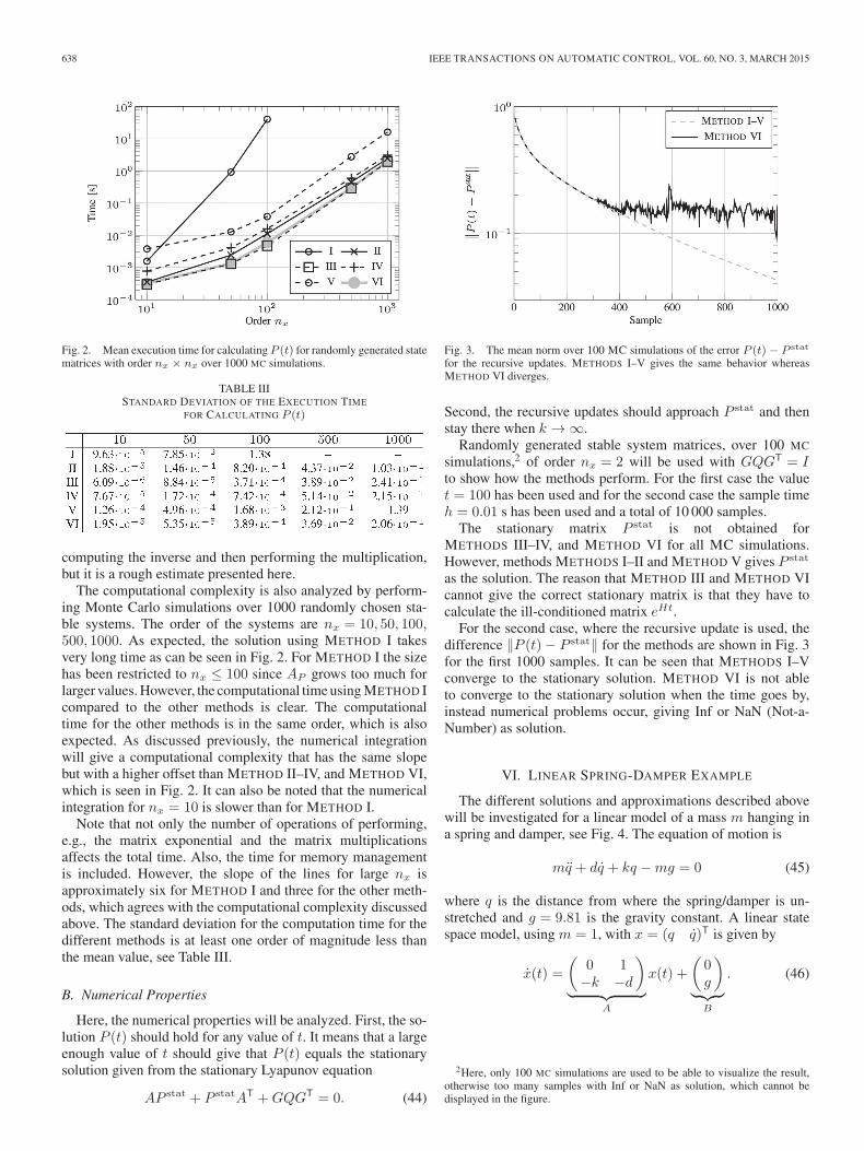
Fig. 2. Mean execution time for calculating P (t) for randomly generated statematrices with order nx × nx over 1000 MC simulations.

TABLE IIISTANDARD DEVIATION OF THE EXECUTION TIME

FOR CALCULATING P (t)

computing the inverse and then performing the multiplication,but it is a rough estimate presented here.

The computational complexity is also analyzed by perform-ing Monte Carlo simulations over 1000 randomly chosen sta-ble systems. The order of the systems are nx = 10, 50, 100,500, 1000. As expected, the solution using METHOD I takesvery long time as can be seen in Fig. 2. For METHOD I the sizehas been restricted to nx ≤ 100 since AP grows too much forlarger values. However, the computational time using METHOD Icompared to the other methods is clear. The computationaltime for the other methods is in the same order, which is alsoexpected. As discussed previously, the numerical integrationwill give a computational complexity that has the same slopebut with a higher offset than METHOD II–IV, and METHOD VI,which is seen in Fig. 2. It can also be noted that the numericalintegration for nx = 10 is slower than for METHOD I.

Note that not only the number of operations of performing,e.g., the matrix exponential and the matrix multiplicationsaffects the total time. Also, the time for memory managementis included. However, the slope of the lines for large nx isapproximately six for METHOD I and three for the other meth-ods, which agrees with the computational complexity discussedabove. The standard deviation for the computation time for thedifferent methods is at least one order of magnitude less thanthe mean value, see Table III.

B. Numerical Properties

Here, the numerical properties will be analyzed. First, the so-lution P (t) should hold for any value of t. It means that a largeenough value of t should give that P (t) equals the stationarysolution given from the stationary Lyapunov equation

AP stat + P statAT +GQGT = 0. (44)

Fig. 3. The mean norm over 100 MC simulations of the error P (t)− P stat

for the recursive updates. METHODS I–V gives the same behavior whereasMETHOD VI diverges.

Second, the recursive updates should approach P stat and thenstay there when k → ∞.

Randomly generated stable system matrices, over 100 MC

simulations,2 of order nx = 2 will be used with GQGT = Ito show how the methods perform. For the first case the valuet = 100 has been used and for the second case the sample timeh = 0.01 s has been used and a total of 10 000 samples.

The stationary matrix P stat is not obtained forMETHODS III–IV, and METHOD VI for all MC simulations.However, methods METHODS I–II and METHOD V gives P stat

as the solution. The reason that METHOD III and METHOD VIcannot give the correct stationary matrix is that they have tocalculate the ill-conditioned matrix eHt.

For the second case, where the recursive update is used, thedifference ‖P (t)− P stat‖ for the methods are shown in Fig. 3for the first 1000 samples. It can be seen that METHODS I–Vconverge to the stationary solution. METHOD VI is not ableto converge to the stationary solution when the time goes by,instead numerical problems occur, giving Inf or NaN (Not-a-Number) as solution.

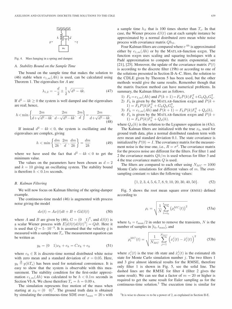
VI. LINEAR SPRING-DAMPER EXAMPLE

The different solutions and approximations described abovewill be investigated for a linear model of a mass m hanging ina spring and damper, see Fig. 4. The equation of motion is

mq + dq + kq −mg = 0 (45)

where q is the distance from where the spring/damper is un-stretched and g = 9.81 is the gravity constant. A linear statespace model, using m = 1, with x = (q q)T is given by

x(t) =

(0 1−k −d

)︸︷︷︸

A

x(t) +

(0g

)︸︷︷︸

B

. (46)

2Here, only 100 MC simulations are used to be able to visualize the result,otherwise too many samples with Inf or NaN as solution, which cannot bedisplayed in the figure.


Fig. 4. Mass hanging in a spring and damper.

A. Stability Bound on the Sample Time

The bound on the sample time that makes the solution to(46) stable when e1,m(Ah) is used, can be calculated usingTheorem 1. The eigenvalues for A are

λ1,2 = −d

2± 1

2

√d2 − 4k. (47)

If d2 − 4k ≥ 0 the system is well damped and the eigenvaluesare real; hence,

h<min

{2m

d+√d2−4k

,2m

d−√d2−4k

,2m

d

}=

2m

d+√d2−4k

.

(48)

If instead d2 − 4k < 0, the system is oscillating and theeigenvalues are complex, giving

h < min

{dm

2k,2m

d,dm

2k

}=

dm

2k(49)

where we have used the fact that d2 − 4k < 0 to get theminimum value.

The values on the parameters have been chosen as d = 2and k = 10 giving an oscillating system. The stability boundis therefore h < 0.1m seconds.

B. Kalman Filtering

We will now focus on Kalman filtering of the spring-damperexample.

The continuous-time model (46) is augmented with processnoise giving the model

dx(t) = Ax(t)dt+B +Gdβ(t) (50)

where A and B are given by (46), G = (0 1)T, and dβ(t) isa scalar Wiener process with E[dβ(t)dβ(t)T] = Qdt. Here itis used that Q = 5 · 10−3. It is assumed that the velocity q ismeasured with a sample rate Ts. The measurement equation canbe written as

yk = (0 1)xk + ek = Cxk + ek (51)

where ek ∈ R is discrete-time normal distributed white noisewith zero mean and a standard deviation of σ = 0.05. Here,yk

Δ= y(kTs) has been used for notational convenience. It is

easy to show that the system is observable with this mea-surement. The stability condition for the first-order approxi-mation e1,m(Ah) was calculated to be h < 0.1m seconds inSection VI-A. We chose therefore Ts = h = 0.09 s.

The simulation represents free motion of the mass whenstarting at x0 = (0 0)T. The ground truth data is obtainedby simulating the continuous-time SDE over tmax = 20 s with

a sample time hS that is 100 times shorter than Ts. In thatcase, the Wiener process dβ(t) can at each sample instance beapproximated by a normal distributed zero mean white noiseprocess with covariance matrix QhS .

Four Kalman filters are compared where eAh is approximatedeither by e1,m(Ah) or by the MATLAB-function expm. Thefunction expm uses scaling and squaring techniques with aPadé approximation to compute the matrix exponential, see[21], [25]. Moreover, the update of the covariance matrix P (t)is according to the discrete filter (19b) or according to one ofthe solutions presented in Section II-A–C. Here, the solution tothe CDLE given by Theorem 5 has been used, but the othermethods would give the same results. Remember though thatthe matrix fraction method can have numerical problems. Insummary, the Kalman filters are as follows.

1) Fh=e1,m(Ah) and P (k + 1)=FhP (k)FTh +GhQhG

Th.

2) Fh is given by the MATLAB-function expm and P (k +1) = FhP (k)FT

h +GhQhGTh,

3) Fh = e1,m(Ah) and P (k + 1) = FhP (k)FTh +Qd(h).

4) Fh is given by the MATLAB-function expm and P (k +1) = FhP (k)FT

h +Qd(h).where Qd(h) is the solution to the Lyapunov equation in (43c).

The Kalman filters are initialized with the true x0, used forground truth data, plus a normal distributed random term withzero mean and standard deviation 0.1. The state covariance isinitialized by P (0) = I . The covariance matrix for the measure-ment noise is the true one, i.e., R = σ2. The covariance matrixfor the process noise are different for the filters. For filter 1 and2 the covariance matrix Qh/m is used whereas for filter 3 and4 the true covariance matrix Q is used.

The filters are compared to each other using NMC = 1000Monte Carlo simulations for different values of m. The over-sampling constant m takes the following values:

{1, 2, 3, 4, 5, 6, 7, 8, 9, 10, 20, 30, 40, 50}. (52)

Fig. 5 shows the root mean square error (RMSE) definedaccording to

ρi =

√√√√ 1

N

tmax∑t=t0

(ρMCi (t)

)2(53a)

where t0 = tmax/2 in order to remove the transients, N is thenumber of samples in [t0, tmax], and

ρMCi (t) =

√√√√ 1

NMC

NMC∑j=1

(xji (t)− xj

i (t))2

(53b)

where xji (t) is the true ith state and xj

i (t) is the estimated ithstate for Monte Carlo simulation number j. The two filters 1and 3 give almost identical results for the RMSE, thereforeonly filter 1 is shown in Fig. 5, see the solid line. Thedashed lines are the RMSE for filter 4 (filter 2 gives thesame result). We can see that a factor of m = 20 or higher isrequired to get the same result for Euler sampling as for thecontinuous-time solution.3 The execution time is similar for

3It is wise to choose m to be a power of 2, as explained in Section II-E.


Fig. 5. RMSE according to (53) as a function of the degree of oversampling,where the solid line is filter 1 (filter 3 gives the same) and the dashed line isfilter 4 (filter 2 gives the same).

Fig. 6. Norm of the stationary covariance matrix for the estimation error forthe four filters, as a function of the degree of oversampling.

all four filters and increases with the same amount when mincreases, hence a large enough oversampling can be difficultto achieve for systems with hard real-time requirements. In thatcase, the continuous-time solution is to prefer.

Remark 6: The maximum sample time, derived according toTheorem 1, is restricted by the CDLE as is described in theproof. It means that we can use a larger sample time for theODE describing the states, in this particular case a twice aslarge sample time. Based on this, we already have oversamplingby a factor of at least two, for the ODE describing the states,when the sample time is chosen according to Theorem 1.

In Fig. 6 we can see how the norm of the stationary covari-ance matrix4 for the estimation error changes when oversam-pling is used. The four filters converge to the same value whenm increases. For the discrete-time update in (19b), i.e., filter 1and 2, the stationary value is too large for small values of m. Forthe continuous-time update in Theorem 5, it can be seen thata first-order Taylor approximation of the exponential function,i.e., filter 3, gives a too small covariance matrix which increaseswhen m increases.

A too small or too large covariance matrix for the estima-tion error can be crucial for different applications, such astarget tracking, where the covariance matrix is used for dataassociation.

4The covariance matrix at time tmax is used as the stationary covariancematrix, i.e., P (tmax).

VII. EXTENSIONS TO NONLINEAR SYSTEMS

We will in this section adapt the results for linear systems tononlinear systems. Inevitably, some approximations have to bedone, and the most fundamental one is to assume that the state isconstant during the small time steps h/m. This approximationbecomes better the larger oversampling factor m is chosen.

A. EKF Time Update

Let the dynamics be given by the nonlinear SDE

dx(t) = f (x(t)) dt+G (x(t)) dβ(t) (54)

for t ≥ 0, where x(t) ∈ Rnx , f(x(t)) : Rnx → R

nx , G(x(t)) :R

nx → Rnx×nβ , and dβ(t) ∈ R

nβ is a vector of Wiener pro-cesses with E[dβ(t)dβ(t)T] = Qdt. For simplicity, it is as-

sumed that G(x(t))Δ= G. The propagation of the first and

second-order moments for the extended Kalman filter (EKF)can, as in the linear case, be written as [2]

˙x(t) = f (x(t)) (55a)

P (t) =F (x(t))P (t) + P (t)F (x(t))T +GQGT (55b)

where F (x(t)) is the Jacobian of f(x(t)) evaluated at x(t). Themain differences to (5) are that a linear approximation of f(x)is used in the CDLE as well as the CDLE is dependent on thestate vector x. Without any assumptions, the two equations in(55) have to be solved simultaneously. The easiest way is tovectorize (55b) similar to what is described in Appendix A andthen solve the nonlinear ODE

d

dt

(x(t)

vechP (t)

)=

(f (x(t)) ,

AP (x(t)) vechP + vechGQGT

)(56)

where AP (x(t)) = D†(I ⊗ F (x(t)) + F (x(t))⊗ I)D. Thenonlinear ODE can be solved using a numerical solver such asRunge–Kutta methods [1]. If it is assumed that x(t) is constantover an interval of length h/m, then the two ODEs describingx(t) and vechP (t) can be solved separately. The ODE for x(t)is solved using a numerical solver and the ODE for vechP (t)becomes a linear ODE which can be solved using Theorem 5,

where AΔ= F (x(t)).

Remark 7: When m increases, the length of the interval,where x(t) has to be constant, decreases. In that case, theassumption of constant x(t) is more valid; hence, the two ODEscan be solved separately without introducing too much errors.

Similar extensions for the method using matrix fraction isstraightforward to derive. The advantage with the vectorisedsolution is that it is easy to solve the combined ODE forx(t) and vechP (t) using a Runge–Kutta solver. This can becompared to the method using matrix fraction, which becomesa coupled differential equation with both vector and matrixvariables.

B. Simulations of a Flexible Joint

A nonlinear model for a single flexible joint is investigatedin this section, see Fig. 7. The equations of motion are given by

Jaqa +G(qa) +D(qa, qm) + T (qa, qm) = 0 (57a)Jmqm + F (qm)−D(qa, qm)− T (qa, qm) =u (57b)


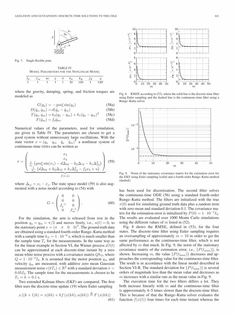
Fig. 7. Single flexible joint.

TABLE IVMODEL PARAMETERS FOR THE NONLINEAR MODEL

where the gravity, damping, spring, and friction torques aremodeled as

G(qa) = −gmξ sin(qa) (58a)D(qa, qm) = d(qa − qm) (58b)T (qa, qm) = k2(qa − qm) + k1(qa − qm)3 (58c)

F (qm) = fdqm. (58d)

Numerical values of the parameters, used for simulation,are given in Table IV. The parameters are chosen to get agood system without unnecessary large oscillations. With thestate vector x = (qa qm qa qm)T a nonlinear system ofcontinuous-time ODEs can be written as

x =

⎛⎜⎜⎝

x3

x41Ja

(gmξ sin(x1)− dΔ34 − k2Δ12 − k1Δ

312

)1

Jm

(dΔ34 + k2Δ12 + k1Δ

312 − fdx4 + u

)⎞⎟⎟⎠

︸︷︷︸f(x,u)

(59)

where Δij = xi − xj . The state space model (59) is also aug-mented with a noise model according to (54) with

G =

⎛⎜⎝

0 00 0

J−1a 00 J−1

m

⎞⎟⎠ . (60)

For the simulation, the arm is released from rest in theposition qa = qm = π/2 and moves freely, i.e., u(t) = 0, tothe stationary point x = (π π 0 0)T. The ground truth dataare obtained using a standard fourth-order Runge–Kutta methodwith a sample time hS = 1 · 10−6 s, which is much smaller thanthe sample time Ts for the measurements. In the same way asfor the linear example in Section VI, the Wiener process dβ(t)can be approximated at each discrete-time instant by a zeromean white noise process with a covariance matrix QhS , whereQ = 1 · 10−3I2. It is assumed that the motor position qm andvelocity qm are measured, with additive zero mean Gaussianmeasurement noise e(kTs) ∈ R

2 with a standard deviation σ =0.05I2. The sample time for the measurements is chosen to beTs = h = 0.1 s.

Two extended Kalman filters (EKF) are compared. The firstfilter uses the discrete-time update (19) where Euler sampling

x ((k + 1)h) = x(kh) + hf (x(kh), u(kh))Δ= F (x(kh))

(61)

Fig. 8. RMSE according to (53), where the solid line is the discrete-time filterusing Euler sampling and the dashed line is the continuous-time filter using aRunge–Kutta solver.

Fig. 9. Norm of the stationary covariance matrix for the estimation error forthe EKF using Euler sampling (solid) and a fourth-order Runge–Kutta method(dashed).

has been used for discretization. The second filter solvesthe continuous-time ODE (56) using a standard fourth-orderRunge–Kutta method. The filters are initialized with the truex(0) used for simulating ground truth data plus a random termwith zero mean and standard deviation 0.1. The covariance ma-trix for the estimation error is initialized by P (0) = 1 · 10−4I4.The results are evaluated over 1000 Monte Carlo simulationsusing the different values of m listed in (52).

Fig. 8 shows the RMSE, defined in (53), for the fourstates. The discrete-time filter using Euler sampling requiresan oversampling of approximately m = 10 in order to get thesame performance as the continuous-time filter, which is notaffected by m that much. In Fig. 9, the norm of the stationarycovariance matrix of the estimation error, i.e., ‖P (tmax)‖, isshown. Increasing m, the value ‖P (tmax)‖ decreases and ap-proaches the corresponding value for the continuous-time filter.The result is in accordance with the linear model described inSection VI-B. The standard deviation for ‖P (tmax)‖ is severalorders of magnitude less than the mean value and decreases asm increases with a similar rate as the mean value in Fig. 9.

The execution time for the two filters differs a lot. Theyboth increase linearly with m and the continuous-time filteris approximately 4–5 times slower than the discrete-time filter.This is because of that the Runge–Kutta solver evaluates thefunction f(x(t)) four times for each time instant whereas the


discrete-time filter evaluates the function F (x(kh)) only once.However, the time it takes for the discrete-time filter usingm = 10 is approximately 1.6 times slower than using m = 1for the continuous-time filter.

VIII. CONCLUSION

This paper investigates the continuous-discrete filtering prob-lem for Kalman filters and extended Kalman filters. The criticaltime update consists of solving one ODE and one continuous-time differential Lyapunov equation (CDLE). The problem canbe rewritten as one ODE by vectorization of the CDLE. Themain contributions of the paper are as follows:

1) A survey of different ways to calculate the covarianceof a linear SDE is presented. The different methods,presented in Table II, are compared to each other withrespect to stability, computational complexity and numer-ical properties.

2) Stability condition for Euler sampling of the linear ODEwhich describes the first- and second-order moments ofthe SDE. An explicit upper bound on the sample timeis derived such that a stable continuous-time systemremains stable after discretization. The stability condi-tion for higher order of approximations, such as theRunge–Kutta method, is also briefly investigated.

3) A numerical stable and time efficient solution to theCDLE that does not require any vectorization. The com-putational complexity for the straightforward solution,using vectorization, of the CDLE is O(n6

x), whereasthe proposed solution, and the methods proposed in theliterature, have a complexity of only O(n3

x).The continuous-discrete filtering problem, using the proposedmethods, is evaluated on a linear model describing a masshanging in a spring-damper pair. It is shown that the standarduse of the discrete-time Kalman filter requires a much highersample rate in order to achieve the same performance as theproposed solution.

The continuous-discrete filtering problem is also extendedto nonlinear systems and evaluated on a nonlinear model de-scribing a single flexible joint of an industrial manipulator. Theproposed solution requires the solution from a Runge–Kuttamethod and without any assumptions, vectorization has to beused for the CDLE. Simulations of the nonlinear joint modelshow also that a much higher sample time is required for thestandard discrete-time Kalman filter to be comparable to theproposed solution.

APPENDIX AVECTORIZATION OF THE CDLE

The matrix valued CDLE

P (t) = AP (t) + P (t)AT +GQGT (62)

can be converted to a vector valued ODE using vectorizationof the matrix P (t). P (t) ∈ R

nx×nx is symmetric so the half-vectorization is used. The relationship between vectorization,denoted by vec, and half-vectorization, denoted by vech, is

vecP (t) = DvechP (t) (63)

where D is a n2x × nx(nx + 1)/2 duplication matrix. Let nP =

nx(nx + 1)/2 and Q = GQGT. Vectorization of (62) gives

vechP (t) = vech(AP (t) + P (t)AT + Q

)=vechAP (t) + vechP (t)AT + vech Q

=D† (vecAP (t) + vecP (t)AT)+ vech Q

(68)= D† [(I ⊗A) + (A⊗ I)]DvechP (t) + vech Q

=APvechP (t) + vech Q (64)

where ⊗ is the Kronecker product and D† = (DTD)−1DT isthe pseudo inverse of D. Note that D†D = I and DD† �= I .The solution of the ODE (64) is given by [20]

vechP (t) = eAP tvechP (0) +

t∫0

eAP (t−s) ds vech Q. (65)

Assume that AP is invertible, then the integral can be com-puted as

t∫0

eAP (t−s) ds = eAP t

t∫0

e−AP s ds

=

/d

ds

(−A−1

P e−AP s)= e−AP s

/= eAP tA−1

P (I − e−AP t) = A−1P (eAP t − I).

(66)

APPENDIX BEIGENVALUES OF THE APPROXIMATED

EXPONENTIAL FUNCTION

The eigenvalues of ep,m(Ah) as a function of the eigenvaluesof A is given in Lemma 8 and Lemma 9 presents the result whenp → ∞ if A is Hurwitz.

Lemma 8: Let λi and vi be the eigenvalues and eigenvectors,respectively, of A ∈ R

n×n. Then the pth-order Taylor expan-sion ep,m(Ah) of eAh is given by

ep,m(Ah) =

(I +

Ah

m+ · · ·+ 1

p!

(Ah

m

)p)m

which has the eigenvectors vi and the eigenvalues(1 +

hλi

m+

h2λ2i

2!m2+

h3λ3i

3!m3+ · · ·+ hpλp

i

p!mp

)m

(67)

for i = 1, . . . , n.Proof: The result follows from an eigenvalue decomposi-

tion of the matrix A. �Lemma 9: In the limit p → ∞, the eigenvalues of ep,m(Ah)

converge to ehλi , i = 1, . . . , n. If A is Hurwitz (Re{λi} < 0),then the eigenvalues are inside the unit circle.

Proof: When p → ∞ the sum in (67) converges to the ex-ponential function ehλi , i = 1, . . . , n. The exponential functioncan be written as

eλih = e�e{λi}h (cos Im{λi}+ i sin Im{λi})

which for Re{λi} < 0 has an absolute value less than 1; hence,eλih is inside the unit circle. �


APPENDIX CRULES FOR VECTORIZATION AND

THE KRONECKER PRODUCT

The rules for vectorization and the Kronecker product arefrom [17] and [23]:

vecAB =(I ⊗A)vecB=(BT ⊗ I)vec (68)

(CT ⊗A)vecB =vecABC (69)I ⊗A+B ⊗ I =A⊕B (70)

eA⊕B = eA ⊗ eB (71)DD†(I ⊗A+A⊗ I)D =(I ⊗A+A⊗ I)D. (72)

ACKNOWLEDGMENT

The authors would like to thank Dr. D. Petersson, LinköpingUniversity, Sweden, for valuable comments regarding matrixalgebra. The authors would also like to thank the reviewers formany constructive comments, in particular one reviewer pro-vided extraordinary contributions to improve the manuscript.

REFERENCES

[1] E. Hairer, S. P. Nørsett, and G. Wanner, Solving Ordinary DifferentialEquations I—Nonstiff Problems. Berlin/Heidelberg, Germany: Springer-Verlag, 1987, ser. Springer Series in Computational Mathematics.

[2] A. H. Jazwinski, Stochastic Processes and Filtering Theory, vol. 64.New York, NY, USA: Academic, 1970.

[3] T. Kailath, A. H. Sayed, and B. Hassibi, Linear Estimation.Upper Saddle River, NJ, USA: Prentice-Hall, 2000, ser. Information andSystem Sciences Series.

[4] J. LaViola, “A comparison of unscented and extended Kalman filteringfor estimating quaternion motion,” in Proc. Amer. Control Conf., Denver,CO, USA, Jun. 2003, pp. 2435–2440.

[5] B. Rao, S. Xiao, X. Wang, and Y. Li, “Nonlinear Kalman filtering withnumerical integration,” Chinese J. Electron., vol. 20, no. 3, pp. 452–456,Jul. 2011.

[6] M. Mallick, M. Morelande, and L. Mihaylova, “Continuous-discrete fil-tering using EKF, UKF, and PF,” in Proc. 15th Int. Conf. Inf. Fusion,Singapore, Jul. 2012, pp. 1087–1094.

[7] J. Bagterp Jörgensen, P. Grove Thomsen, H. Madsen, and M. RodeKristensen, “A computational efficient and robust implementation ofthe continuous-discrete extended Kalman filter,” in Proc. Amer. ControlConf., New York, NY, USA, Jul. 2007, pp. 3706–3712.

[8] T. Mazzoni, “Computational aspects of continuous-discrete extendedKalman-filtering,” Comput. Statist., vol. 23, no. 4, pp. 519–539, 2008.

[9] P. Frogerais, J.-J. Bellanger, and L. Senhadji, “Various ways to computethe continuous-discrete extended Kalman filter,” IEEE Trans. Autom.Control, vol. 57, no. 4, pp. 1000–1004, Apr. 2012.

[10] S. Särkkä, “On unscented Kalman filtering for state estimation ofcontinuous-time nonlinear systems,” IEEE Trans. Autom. Control, vol. 52,no. 9, pp. 1631–1641, Sep. 2007.

[11] ONP. Zhang, J. Gu, E. Milios, and P. Huynh, “Navigation with IMU/GPS/digital compass with unscented Kalman filter,” in Proc. IEEEInt. Conf. Mechatron. Autom., Niagara Falls, Canada, Jul./Aug. 2005,pp. 1497–1502.

[12] I. Arasaratnam and S. Haykin, “Cubature Kalman filtering: A powerfultool for aerospace applications,” in Proc. Int. Radar Conf., Bordeaux,France, Oct. 2009.

[13] C. F. Van Loan, “Computing integrals involving the matrix exponential,”IEEE Trans. Autom. Control, vol. AC-23, no. 3, pp. 395–404, Jun. 1978.

[14] M. S. Grewal and A. P. Andrews, Kalman Filtering. Theory and PracticeUsing Matlab, 3rd ed. Hoboken, NJ, USA: Wiley, 2008.

[15] S. Särkkä, “Recursive Bayesian inference on stochastic differential equa-tions,” Ph.D. dissertation, Helsinki Univ. of Technol., Helsinki, Finland,Apr., 2006, ISBN: 9-512-28127-9.

[16] H. J. Rome, “A direct solution to the linear variance equation of a time-invariant linear system,” IEEE Trans. Autom. Control, vol. AC-14, no. 5,pp. 592–593, Oct. 1969.

[17] N. J. Higham, Functions of Matrices—Theory and Computation.Philadelphia, PA, USA: SIAM, 2008.

[18] E. J. Davison, “The numerical solution of X = A1X +XA2 +D,X(0) = C,” IEEE Trans. Autom. Control, vol. AC-20, no. 4, pp. 566–567, Aug. 1975.

[19] Z. Gajicc and M. T. J. Qureshi, Lyapunov Matrix Equation in SystemStability and Control, vol. 195. San Diego, CA, USA: Academic, 1995,ser. Mathematics in Science and Engineering.

[20] W. J. Rugh, Linear System Theory, 2nd ed. Upper Saddle River, NJ,USA: Prentice-Hall, 1996, ser. Information and System Sciences Series.

[21] C. Moler and C. Van Loan, “Nineteen dubious ways to compute theexponential of a matrix, twenty-five years later,” SIAM Rev., vol. 45, no. 1,pp. 1–46, Feb. 2003.

[22] D. Hinrichsen and A. J. Pritchard, Mathematical Systems Theory I—Modelling, State Space Analysis, Stability and Robustness. Berlin/Heidelberg, Germany: Springer-Verlag, 2005, ser. Texts in AppliedMathematics.

[23] H. Lütkepohl, Handbook of Matrices. Chichester, U.K.: Wiley, 1996.[24] N. Wahlström, P. Axelsson, and F. Gustafsson, “Discretizing stochastic

dynamical systems using Lyapunov equations,” in Proc. 19th IFAC WorldCongr., Cape Town, South Africa, Aug. 2014.

[25] N. J. Higham, “The scaling and squaring method for the matrix exponen-tial revisited,” SIAM J. Matrix Anal. Applicat., vol. 26, no. 4, pp. 1179–1193, Jun. 2005.

Patrik Axelsson received the M.Sc. degree in ap-plied physics and electrical engineering and thePh.D. degree in automatic control from LinköpingUniversity, Linköping, Sweden, in January 2009 andMay 2014, respectively.

His research interests include sensor fusion andcontrol applied to industrial manipulators, with afocus on nonlinear flexible joint models.

Fredrik Gustafsson (F’12) received the M.Sc. de-gree in electrical engineering and the Ph.D. de-gree in automatic control from Linköping University,Linköping, Sweden, in 1988 and 1992, respectively.

He has been a Professor in sensor informatics inthe Department of Electrical Engineering, LinköpingUniversity, since 2005. From 1992 to 1999, he heldvarious positions in automatic control, and from1999 to 2005 he had a professorship in communi-cation systems. His research interests are in stochas-tic signal processing, adaptive filtering, and change

detection, with applications to communication, vehicular, airborne, and audiosystems. He is a cofounder of the companies NIRA Dynamics (automotivesafety systems), Softube (audio effects), and SenionLab (indoor positioningsystems).

He was an associate editor for the IEEE TRANSACTIONS OF SIGNAL

PROCESSING (2000–2006), IEEE TRANSACTIONS ON AEROSPACE AND

ELECTRONIC SYSTEMS (2010–2012), and EURASIP Journal on Applied Sig-nal Processing (2007–2012). He was awarded the Arnberg prize by the RoyalSwedish Academy of Science (KVA) in 2004, elected member of the RoyalAcademy of Engineering Sciences (IVA) in 2007, elevated to IEEE Fellowin 2011 and awarded the Harry Rowe Mimno Award in 2011 for the tutorial“Particle Filter Theory and Practice with Positioning Applications,” which waspublished in the AESS Magazine in July 2010.

06887356

Documents