06125556
TRANSCRIPT

7/14/2019 06125556
http://slidepdf.com/reader/full/06125556 1/6
Switching transients in long AC cable connections to
offshore wind farmsF. Moore
Cardiff [email protected]
A. HaddadCardiff [email protected]
H. GriffithsCardiff University
M. Osborne National Grid UK
Abstract- Overvoltages arising from energising a 45km132kV submarine cable connection to an offshore wind farmwere calculated using EMTP. Energisation of the submarinecable and remote 132/33kV transformer connected as atransformer-feeder was first simulated. The resultingovervoltages were compared with overvoltages caused byenergising the cable and transformer separately.
Index Terms-- ATP, ATPDraw, Cables, EMTP, Offshore,Overvoltage, Switching, Transients, Wind
I. I NTRODUCTION
In the UK, there are currently over 30GW of offshore
wind generation projects at various stages of development[1]. These result from government targets and incentives for
renewable energy [3][4]. The location of these large wind
farms means that long lengths of submarine cable are
required to connect the wind farms to the onshore
transmission network. It is important to investigate how these
long lengths of cable will influence the transient overvoltages
seen on the onshore transmission network.
Figure 1 shows a 33kV wind farm array connected to the
400kV onshore transmission system using 132kV submarine
cables.
Offshore
Substation
132/33kV
Onshore
Interface
Substation
(400/132kV)
Submarine
Cables (132kV)
Onshore Transmission Network (400kV)
To Wind Farm (33kV)
Offshore
Substation
132/33kV
Onshore
Interface
Substation
(400/132kV)
Submarine
Cables (132kV)
Onshore Transmission Network (400kV)
To Wind Farm (33kV)
Figure 1 Typical Offshore Network Configuration (Compensation plant
and harmonic filters at 400/132kV interface substation are omitted for
clarity)
The design of this offshore network requires a trade off
between cost and operability. Reducing plant on the offshore
platform substation has significant cost benefits. The
132/33kV offshore transformers could potentially be
connected directly to the 132kV submarine cables as
transformer-feeders, removing the need for 132kV circuit
breakers in the offshore substation.
This paper describes the development of a computer model
for the AC connection to an offshore wind farm. This paper
focuses on the overvoltages arising from energisation of wind
farm connection. Energisation of the submarine cable and
offshore 132/33kV transformer together as a transformer-
feeder is compared with energising the two items separately.
II. OFFSHORE CONNECTION MODEL
Figure 2 shows a model in ATPDraw, for the interface
between offshore and onshore transmission networks.
Network
Source
400/132/13kV
Transformer
400kV OHL
(Double Circuit)
400kV OHL
(Double Circuit)
Network
Source
Harmonic
Filter
13kV Shunt Reactor
Network Interface
Onshore 132kV Circuit Breaker
132kV Submarine Cable (45km)
Offshore 132kV Circuit Breaker
132/33kV
Transformer
Zy Earthing
Transformer
V V
V
V
V
V
V
V
Network
Source
400/132/13kV
Transformer
400kV OHL
(Double Circuit)
400kV OHL
(Double Circuit)
Network
Source
Harmonic
Filter
13kV Shunt Reactor
Network Interface
Onshore 132kV Circuit Breaker
132kV Submarine Cable (45km)
Offshore 132kV Circuit Breaker
132/33kV
Transformer
Zy Earthing
Transformer
V V
V
V
V
V
V
V
Figure 2 Offshore Connection Model in ATPDraw with a 400kV
Onshore Network. (Lettered circles mark where voltage measurements
were taken during simulations.)
A single 132kV submarine circuit, similar to those shown
in Figure 1, is modelled to allow energisation studies to be
carried out. The different aspects of the model are detailed in
the following section. No overvoltage protection was
included in the model.
UPEC 2011 ∙ 46th International Universities' Power Engineering Conference ∙ 5-8th September 2011 ∙ Soest ∙ Germany
ISBN 978-3-8007-3402-3 © VDE VERLAG GMBH ∙ Berlin ∙ Offenbach
7/14/2019 06125556
http://slidepdf.com/reader/full/06125556 2/6
A. 400kV Onshore Network
The onshore transmission system is represented using two
network equivalents connected by a 400kV double circuit
overhead line. The offshore wind farm is connected by
turning in one of the 400kV overhead circuits.
Each network equivalent is a voltage source behind an
impedance comprising; an inductance, representing the
network fault level in parallel with a resistance representingthe network surge impedance. It was assumed that the fault
level contribution is shared equally between the two
equivalent sources. The network fault level is assumed to be
17.5GVA, or just over 25kA which is typical for the UK
Transmission system [4].
B. Transformers and Earthing
There are two power transformers represented in the
model; the 400/132/13kV (Yyd) autotransformer at the
onshore substation and the 132/33kV (Yd) transformer at the
offshore substation. Both are modelled using the BCTRAN
component. Saturation is represented using nonlinear
inductors connected to the lowest voltage winding in eachtransformer. Core losses are modelled as resistances within
each BCTRAN component. Winding capacitances are
connected externally.
Earthing transformers are installed on the 33kV side of the
132/33kV transformer to provide an earth to the delta
connected 33kV network. These are Zy transformers, which
are also used to supply power to the platform substation. The
earthing method used in this model is similar to that in
Lillegrund Wind Farm [5]; a 130kVA Zy transformer with
zero sequence impedance of 30ȍ is connected with a 67 ȍ
resistance between the neutral point and earth.
The 33/0.415kV Zy transformer is represented using the
Saturable Transformer component, with winding impedances
calculated from test certificate measurements according to
[6]. Saturation of the Zy transformer has been ignored, and
the flux-current relationship is linear; represented by a single
point based on the magnetising current.
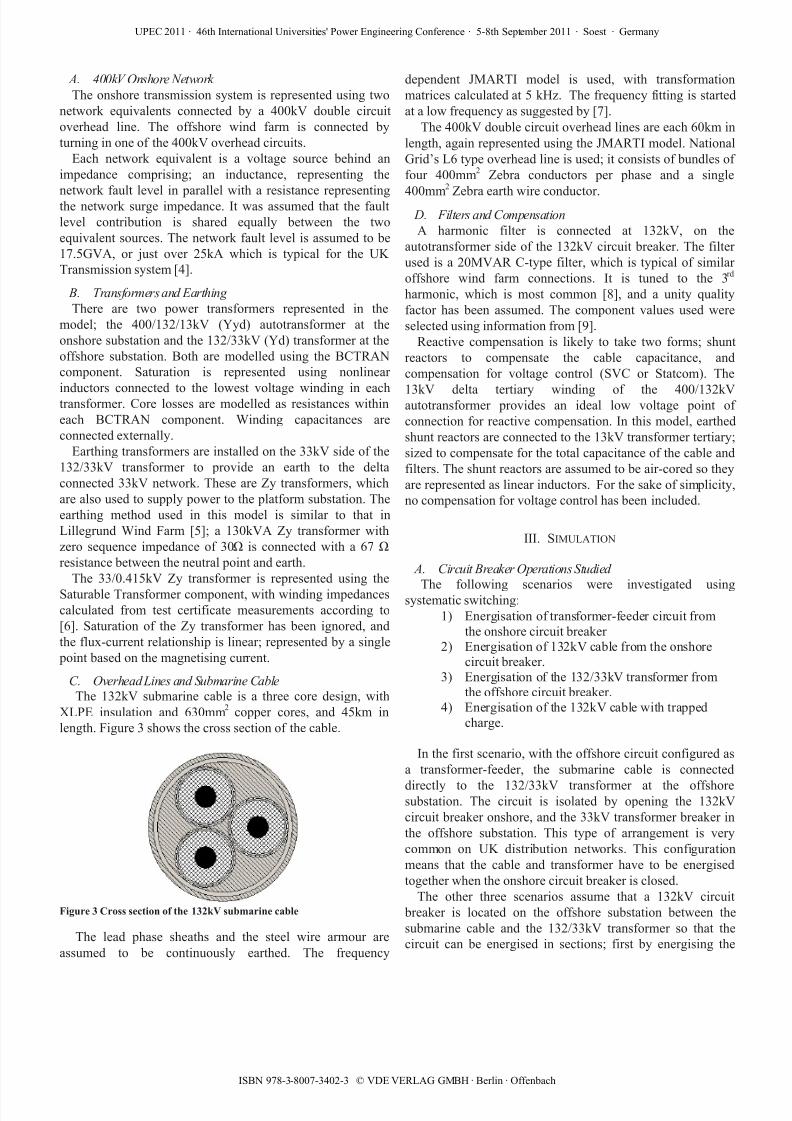
C. Overhead Lines and Submarine CableThe 132kV submarine cable is a three core design, with
XLPE insulation and 630mm2
copper cores, and 45km in
length. Figure 3 shows the cross section of the cable.
Figure 3 Cross section of the 132kV submarine cable
The lead phase sheaths and the steel wire armour are
assumed to be continuously earthed. The frequency
dependent JMARTI model is used, with transformation
matrices calculated at 5 kHz. The frequency fitting is started
at a low frequency as suggested by [7].
The 400kV double circuit overhead lines are each 60km in
length, again represented using the JMARTI model. National
Grid’s L6 type overhead line is used; it consists of bundles of
four 400mm2 Zebra conductors per phase and a single
400mm
2
Zebra earth wire conductor. D. Filters and Compensation
A harmonic filter is connected at 132kV, on the
autotransformer side of the 132kV circuit breaker. The filter
used is a 20MVAR C-type filter, which is typical of similar
offshore wind farm connections. It is tuned to the 3rd
harmonic, which is most common [8], and a unity quality
factor has been assumed. The component values used were
selected using information from [9].
Reactive compensation is likely to take two forms; shunt
reactors to compensate the cable capacitance, and
compensation for voltage control (SVC or Statcom). The
13kV delta tertiary winding of the 400/132kVautotransformer provides an ideal low voltage point of
connection for reactive compensation. In this model, earthed
shunt reactors are connected to the 13kV transformer tertiary;
sized to compensate for the total capacitance of the cable and
filters. The shunt reactors are assumed to be air-cored so they
are represented as linear inductors. For the sake of simplicity,
no compensation for voltage control has been included.
III. SIMULATION
A. Circuit Breaker Operations Studied
The following scenarios were investigated usingsystematic switching:
1) Energisation of transformer-feeder circuit from
the onshore circuit breaker 2) Energisation of 132kV cable from the onshore
circuit breaker.3) Energisation of the 132/33kV transformer from
the offshore circuit breaker.4) Energisation of the 132kV cable with trapped
charge.
In the first scenario, with the offshore circuit configured as
a transformer-feeder, the submarine cable is connected
directly to the 132/33kV transformer at the offshoresubstation. The circuit is isolated by opening the 132kV
circuit breaker onshore, and the 33kV transformer breaker in
the offshore substation. This type of arrangement is very
common on UK distribution networks. This configuration
means that the cable and transformer have to be energised
together when the onshore circuit breaker is closed.
The other three scenarios assume that a 132kV circuit
breaker is located on the offshore substation between the
submarine cable and the 132/33kV transformer so that the
circuit can be energised in sections; first by energising the
UPEC 2011 ∙ 46th International Universities' Power Engineering Conference ∙ 5-8th September 2011 ∙ Soest ∙ Germany
ISBN 978-3-8007-3402-3 © VDE VERLAG GMBH ∙ Berlin ∙ Offenbach

7/14/2019 06125556
http://slidepdf.com/reader/full/06125556 3/6
132kV cable from the onshore circuit breaker, then by closing
the offshore 132kV circuit breaker to energise the 132/33kV
transformer.
When the 132kV cable can be de-energised without the
transformer attached to the remote end, there is a likelihood
of leaving a trapped charge on the cable (provided there is no
circuit component to provide a discharge path to earth). A
trapped charge was introduced to the simulation by startingthe simulation with the onshore circuit breaker closed towards
the 132kV cable. After 1ms the circuit breaker is opened. The
circuit breaker is modelled as an ideal switch which opens
when the cable charging current is zero, leaving a voltage
remaining on the cable (in this case, phase B is left at 1pu,
phases A and C are left at -1pu). The magnitude of this
trapped charge is extreme, and represents the worst case when
re-closing the onshore circuit breaker onto the cable.
B. Statistical Switching Statistical switching was used to determine the range of
overvoltages from different circuit breaker pole closing times
across the 20ms/50Hz waveform. Switching across one thirdor half of the waveform would probably be acceptable if
symmetry is assumed; however, trapped charge is explored
by simulating a single breaker opening event prior to
statistically re-closing the circuit breaker. In this case,
switching across the whole waveform is required.
The approach taken for the simulations described in this
paper is similar to that used in [10] and the dependent model
described in [11]. A master switch determines the instant at
which circuit breaker closing is initiated. The closing time of
this master contact varies according to the uniform
distribution over a range of 0 to 1/ f . After the master switch
closes, each of the three associated phase contacts closes after
an average delay of 20ms. This delay is varied according to
the Gaussian distribution, with a standard deviation of
0.833ms corresponding to a maximum pole span of 5ms. The
end result is random switching events spread across one 20ms
waveform, centered on 30ms.
A total of 3500 operations were simulated for each circuit
breaker operation studied. In order to ensure the results were
directly comparable, the same statistical switching times were
used for each switching scenario studied.
IV. R ESULTS: STATISTICAL
Table 1 summarises the highest overvoltages found at each
network for the four different energisation events simulated.The overvoltages are calculated as per unit quantities; the unit
voltages used are the peak AC voltages shown in Table 2 . It
can be seen that the highest overvoltages of all were seen at
the 13kV tertiary winding of the 400/132kV autotransformer.
These overvoltages occurred whenever the cable was
energised.
Table 1 - The highest overvoltages found at the different network
voltages during statistical switching simulations.
Transformer-Feeder
(Cable & 132/33kV
Transformer)
132kV Cable 132/33kV Transformer 132kV Cable (with
Trapped Charge)
400kV 1.15 1.15 1.05 1.25
132kV 1.95 1.85 1.9 2.75
33kV 1.85 NA 2.6 NA
13kV 5.2 3.8 1.2 8.75
Network
Voltage
Plant Energised
The highest overvoltages seen on the 33kV network, 2.6pu,
occurred when the 132/33kV transformer was energised by
the closing of the offshore 132kV circuit breaker.
The maximum overvoltages seen by the 132kV network
were consistently around 1.9pu, for all operations except the
energisation with trapped charge. Energising the 132kV cable
with trapped charge produced greater overvoltages of up to
2.75pu on the 132kV system.
Under all energisation operations, little impact was seen
on the 400kV transmission network. The results of the
statistical simulations for each scenario are shown as
cumulative probability curves in Figure 4. The results showthe distribution of the overvoltages calculated using statistical
switching.
The minimum standard rated switching impulse withstand
voltage (SIWV) is 850kV for the insulation used on the
400kV transmission network [12]. This equates to 2.6pu,
whilst the highest overvoltage seen on the 400kV was only
1.25pu.
Standard SIWV voltages for 132kV, 33kV and 13kV are
not directly listed IEC 60071-1. The SIWV needs to be
calculated applying a test conversion factor to the standard
corresponding lightning impulse withstand voltages (LIWV)
[12]. This test conversion factor depends on the insulation
type. By dividing the LIWV by the test conversion factor of
1.25 for GIS, and then a safety factor of 1.15, we can
calculate the SIWV. Using the test conversion factor for GIS
will give more conservative answers than other insulation
media. A safety factor of 1.15 is used for enclosed insulation
systems. Table 2 summarizes the relevant insulation
strengths.
Table 2 Standard insulation strengths taken from IEC 60071 [12][13],
alongside corresponding pu values.
V o l t a g e ( L - L ,
k V )
U n i t V o l t a g e ( k V ,
p e a k )
S h o r t D u r a
t i o n P o w e r
F r e q u e n c y
W i t h s t a n d
( k V , r m s )
S I W V ( k V ,
p e a k )
L I W V ( k V , p e a k )
S h o r t D u r a
t i o n P o w e r
F r e q u e n c y
W i t h s t a n d
( P U ) *
S I W V ( p u ) *
*
400kV 326.6 NA 850-950 1050-1425 NA NA
132kV 107.8 275 NA 650 3.6 4.2
33kV 26.9 70 NA 170 3.7 4.4
13kV 10.6 38 NA 95 5.1 6.23
**Calculated by dividing LIWV by test conversion factor (1.25) and by safety factor
(1.15), then by refering to the base voltage.
*RMS values of short duration power frequency withstand voltages have been
given a pu value by assuming they are sinusiodal AC, and referring them to the
unit voltage.
UPEC 2011 ∙ 46th International Universities' Power Engineering Conference ∙ 5-8th September 2011 ∙ Soest ∙ Germany
ISBN 978-3-8007-3402-3 © VDE VERLAG GMBH ∙ Berlin ∙ Offenbach

7/14/2019 06125556
http://slidepdf.com/reader/full/06125556 4/6
0
20
40
60
80
100
120
1 1.5 2 2.5 3 3.5 4 4.5 5 5.5
Voltage (pu)
C u m u l a t i v e P r o b a b i l i t y ( % )
0
20
40
60
80
100
120
1 1.5 2 2.5 3 3.5 4
Voltage (pu)
C u m u l a t i v e P r o b a b i l i t y ( % )
0
20
40
60
80
100
120
1 1.5 2 2.5 3 3.5 4 4.5 5 5.5 6 6.5 7 7.5 8 8.5 9
Voltage (pu)
C u m u l a t i v
e P r o b a b i l i t y ( % )
0
20
40
60
80
100
120
1 1.5 2 2.5 3
Voltage (pu)
C u m u l a t i v e P r o b a b i l i t y ( % )
400kV
132kV
33kV
13kV
Transformer-feeder
132kV Cable
132/33kV
Transformer
132kV Cable
with TrappedCharge
0
20
40
60
80
100
120
1 1.5 2 2.5 3 3.5 4 4.5 5 5.5
Voltage (pu)
C u m u l a t i v e P r o b a b i l i t y ( % )
0
20
40
60
80
100
120
1 1.5 2 2.5 3 3.5 4
Voltage (pu)
C u m u l a t i v e P r o b a b i l i t y ( % )
0
20
40
60
80
100
120
1 1.5 2 2.5 3 3.5 4 4.5 5 5.5 6 6.5 7 7.5 8 8.5 9
Voltage (pu)
C u m u l a t i v
e P r o b a b i l i t y ( % )
0
20
40
60
80
100
120
1 1.5 2 2.5 3
Voltage (pu)
C u m u l a t i v e P r o b a b i l i t y ( % )
400kV
132kV
33kV
13kV
400kV
132kV
33kV
13kV
Transformer-feeder
132kV Cable
132/33kV
Transformer
132kV Cable
with TrappedCharge
Figure 4 Cumulative probability curves of overvoltages calculated for
different voltages on the network using the statistical energisation
studies.
V. R ESULTS: WAVEFORMS
This section shows waveforms resulting from randomly
generated switching operation 431, which resulted in circuit
breaker poles closing at 33.6ms, 36ms, and 36.9ms for each
scenario studied.Figure 5 shows the voltages at various points during the
energisation of the circuit as a transformer-feeder. As the
circuit breaker poles close onto the uncharged 132kV cable,
there is instantaneous depression in voltage on the 132kV
side of the 400/132/13kV transformer, this can be seen in
Figure 5B. The sudden change in voltage on the 132kV
terminals, results in significant overvoltages being introduced
to the 13kV tertiary winding due to the capacitive coupling
between the windings. This can be seen in Figure 5C.
(A) Onshore Transformer 400kV Terminals
(B) Onshore Transformer 132kV Terminals
30 35 40 45 50 55 60 65 70-40
-30
-20
-10
0
10
20
30
V o l t a g e [ k V ]
Time [ms]
(C) Onshore Transformer 13kV Terminals
(b)
30 35 40 45 50 55 60 65 70-200
-100
0
100
200
V o l t a g e [ k V ]
V o l t
a g e [ k V ]
30 35 40 45 50 55 60 65 70-45
-30
-15
0
15
30
45
Time [ms] Time [ms]
(E) Offshore Transformer 33kV Terminals
(D) Offshore Transformer 132kV Terminals
(a)
30 35 40 45 50 55 60 65 70-400
-200
0
200
400
V o l t a g e [ k V ]
30 35 40 45 50 55 60 65 70-200
-100
0
100
200
V o l t a g e [ k V ]
Time [ms] Time [ms]
(A) Onshore Transformer 400kV Terminals
(B) Onshore Transformer 132kV Terminals
30 35 40 45 50 55 60 65 70-40
-30
-20
-10
0
10
20
30
V o l t a g e [ k V ]
Time [ms]30 35 40 45 50 55 60 65 70
-40
-30
-20
-10
0
10
20
30
V o l t a g e [ k V ]
Time [ms]
(C) Onshore Transformer 13kV Terminals
(b)
30 35 40 45 50 55 60 65 70-200
-100
0
100
200
V o l t a g e [ k V ]
V o l t
a g e [ k V ]
30 35 40 45 50 55 60 65 70-45
-30
-15
0
15
30
45
Time [ms] Time [ms]
(b)
30 35 40 45 50 55 60 65 70-200
-100
0
100
200
V o l t a g e [ k V ]
V o l t
a g e [ k V ]
30 35 40 45 50 55 60 65 70-45
-30
-15
0
15
30
45
(b)
30 35 40 45 50 55 60 65 70-200
-100
0
100
200
V o l t a g e [ k V ]
V o l t
a g e [ k V ]
30 35 40 45 50 55 60 65 70-45
-30
-15
0
15
30
45
Time [ms] Time [ms]
(E) Offshore Transformer 33kV Terminals
(D) Offshore Transformer 132kV Terminals
(a)
30 35 40 45 50 55 60 65 70-400
-200
0
200
400
V o l t a g e [ k V ]
30 35 40 45 50 55 60 65 70-200
-100
0
100
200
V o l t a g e [ k V ]
Time [ms] Time [ms]
(a)
30 35 40 45 50 55 60 65 70-400
-200
0
200
400
V o l t a g e [ k V ]
30 35 40 45 50 55 60 65 70-200
-100
0
100
200
V o l t a g e [ k V ]
(a)
30 35 40 45 50 55 60 65 70-400
-200
0
200
400
V o l t a g e [ k V ]
30 35 40 45 50 55 60 65 70-200
-100
0
100
200
V o l t a g e [ k V ]
Time [ms] Time [ms]
Figure 5 Voltage waveforms during transformer-feeder energisation
using onshore 132kV CB (Results shown for poles closing at 33.6ms,
36ms, and 36.9ms)
The high frequency oscillation in Figure 5C is a result of
oscillation between the coupling capacitance and the shunt
reactors. The oscillation is removed when the shunt reactors
were separated from the transformer tertiary winding by a
length of cable, although the initial voltage spike was still
apparent. Further work is probably needed to ensure that the
capacitive coupling between windings is accurately
represented.
Figure 6 shows the waveforms as the 132kV cable is
energised on its own. The behaviour is largely similar to the
scenario with the transformer-feeder energisation. The 132kV
waveforms from the transformer-feeder energisation in Figure5 show some additional distortion due to saturation of the
transformer during inrush.
(A) Onshore Transformer 400kV Terminals
Time [ms]
(B) Onshore Transformer 132kV Terminals
Time [ms] Time [ms]
(D) Offshore End of 132kV Cable
(C) Onshore Transformer 13kV TerminalsTime [ms]
30 35 40 45 50 55 60 65 70-400
-200
0
200
400
30 35 40 45 50 55 60 65 70-30
-20
-10
0
10
20
30
V o l t a g e [ k V ]
V o l t a g e
[ k V ]
30 35 40 45 50 55 60 65 70-200
-100
0
100
200
30 35 40 45 50 55 60 65 70-160
-80
0
80
160
V o l t a g e [ k V ]
V o l t a g e [ k V ]
(A) Onshore Transformer 400kV Terminals
Time [ms]
(B) Onshore Transformer 132kV Terminals
Time [ms] Time [ms]
(D) Offshore End of 132kV Cable
(C) Onshore Transformer 13kV TerminalsTime [ms]
30 35 40 45 50 55 60 65 70-400
-200
0
200
400
30 35 40 45 50 55 60 65 70-30
-20
-10
0
10
20
30
V o l t a g e [ k V ]
V o l t a g e
[ k V ]
30 35 40 45 50 55 60 65 70-400
-200
0
200
400
30 35 40 45 50 55 60 65 70-400
-200
0
200
400
30 35 40 45 50 55 60 65 70-30
-20
-10
0
10
20
30
30 35 40 45 50 55 60 65 70-30
-20
-10
0
10
20
30
V o l t a g e [ k V ]
V o l t a g e
[ k V ]
30 35 40 45 50 55 60 65 70-200
-100
0
100
200
30 35 40 45 50 55 60 65 70-160
-80
0
80
160
V o l t a g e [ k V ]
V o l t a g e [ k V ]
30 35 40 45 50 55 60 65 70-200
-100
0
100
200
30 35 40 45 50 55 60 65 70-200
-100
0
100
200
30 35 40 45 50 55 60 65 70-160
-80
0
80
160
V o l t a g e [ k V ]
V o l t a g e [ k V ]
Figure 6 Voltage waveforms during 132kV cable energisation using
onshore 132kV CB. (Results shown for poles closing at 33.6s, 36ms, and
36.9ms)
Figure 7 shows the voltage waveforms when 132/33kV
transformer is energised from the 132kV offshore circuit
breaker. Unlike Figure 5B, little voltage depression is
apparent on the 132kV terminal of the 400/132/13kV
UPEC 2011 ∙ 46th International Universities' Power Engineering Conference ∙ 5-8th September 2011 ∙ Soest ∙ Germany
ISBN 978-3-8007-3402-3 © VDE VERLAG GMBH ∙ Berlin ∙ Offenbach

7/14/2019 06125556
http://slidepdf.com/reader/full/06125556 5/6
transformer in Figure 7B. The distortion visible here is
harmonic distortion due to transformer inrush. Figure 7D and
Figure 7E show high frequency oscillations as the 132/33kV
transformer being energised one pole at a time.
(A) Onshore Transformer 400kV TerminalsTime [ms]
(B) Onshore Transformer 132kV Terminals
Time [ms]
Time [ms]
(C) Onshore Transformer 13kV Terminals
Time [ms]
(E) Offshore Transformer 33kV Terminals
(D) Offshore Transformer 132kV TerminalsTime [ms]
30 35 40 45 50 55 60 65 70-400
-200
0
200
400
30 35 40 45 50 55 60 65 70-200
-150
-100
-50
0
50
100
150
V o
l t a g e [ k V ]
V o
l t a g e [ k V ]
30 35 40 45 50 55 60 65 70-150
-100
-50
0
50
100
150
30 35 40 45 50 55 60 65 70-60
-40
-20
0
20
40
60
V o l t a g e [ k V ]
V o l t a g e [ k V ]
30 35 40 45 50 55 60 65 70-12
-8
-4
0
4
8
V o l t a g e [ k V ]
(A) Onshore Transformer 400kV TerminalsTime [ms]
(B) Onshore Transformer 132kV Terminals
Time [ms]
Time [ms]
(C) Onshore Transformer 13kV Terminals
Time [ms]
(E) Offshore Transformer 33kV Terminals
(D) Offshore Transformer 132kV TerminalsTime [ms]
30 35 40 45 50 55 60 65 70-400
-200
0
200
400
30 35 40 45 50 55 60 65 70-400
-200
0
200
400
30 35 40 45 50 55 60 65 70-200
-150
-100
-50
0
50
100
150
30 35 40 45 50 55 60 65 70-200
-150
-100
-50
0
50
100
150
V o
l t a g e [ k V ]
V o
l t a g e [ k V ]
30 35 40 45 50 55 60 65 70-150
-100
-50
0
50
100
150
30 35 40 45 50 55 60 65 70-60
-40
-20
0
20
40
60
V o l t a g e [ k V ]
V o l t a g e [ k V ]
30 35 40 45 50 55 60 65 70-12
-8
-4
0
4
8
V o l t a g e [ k V ]
Figure 7 Voltage waveforms during 132/33kV transformer energisation
using offshore 132kV CB. (Results shown for poles closing at 33.6ms,
36ms, and 36.9ms)
Figure 8 shows the waveforms as the 132kV cable is
energised with trapped charge. The behaviour is largely
similar to the scenario with the 132kV cable energised
without trapped charge; however, the overvoltages are more
extreme.
30 35 40 45 50 55 60 65 70-300
-200
-100
0
100
200
300
V o l t a g e [ k V ]
30 35 40 45 50 55 60 65 70-300
-200
-100
0
100
200
300
V o l t a g e [ k V ]
30 35 40 45 50 55 60 65 70-400
-200
0
200
V o l t a g e [ k V ]
30 35 40 45 50 55 60 65 70-60
-40
-20
0
20
40
60
V o l t a g e [ k V
]
(A) Onshore Transformer 400kV Terminals
Time [ms]
(B) Onshore Transformer 132kV Terminals
Time [ms] Time [ms]
(D) Offshore End of 132kV Cable
(C) Onshore Transformer 13kV TerminalsTime [ms]
30 35 40 45 50 55 60 65 70-300
-200
-100
0
100
200
300
30 35 40 45 50 55 60 65 70-300
-200
-100
0
100
200
300
V o l t a g e [ k V ]
30 35 40 45 50 55 60 65 70-300
-200
-100
0
100
200
300
V o l t a g e [ k V ]
30 35 40 45 50 55 60 65 70-400
-200
0
200
V o l t a g e [ k V ]
30 35 40 45 50 55 60 65 70-60
-40
-20
0
20
40
60
V o l t a g e [ k V
]
(A) Onshore Transformer 400kV Terminals
Time [ms]
(B) Onshore Transformer 132kV Terminals
Time [ms] Time [ms]
(D) Offshore End of 132kV Cable
(C) Onshore Transformer 13kV TerminalsTime [ms]
Figure 8 Voltage waveforms during energisation of 132kV cable with
trapped charge using onshore 132kV CB. (Locations shown are letteredas in Figure 2. Results shown for poles closing at 33.6mS, 36mS, and
36.9mS)
VI. CONCLUSIONS
Overvoltages on the 132kV and 400kV systems caused by
energising the submarine cable together with the 132/33kV
transformer were of similar magnitudes to those caused when
the cable and transformer were energised separately.
Energising the 132/33kV transformer separately using a
circuit breaker located offshore caused greater overvoltages
on the 33kV system.
Transformer-feeder circuits are common on UK
distribution networks because of the reduced number of
circuit breakers required. On the offshore platform, where
space and weight are at a premium, this is particularly
desirable. One crucial difference is that on the offshore
transformer, the 132kV cable connection to the transformer
would likely be enclosed due to space restrictions on the
platform, rather than terminated using open bushings. Thiscould potentially be difficult operationally, as flexible earths
cannot then be applied to earth the transformer HV locally.
Under all scenarios considered, little effect was seen on the
400kV system. Even in the extreme case of trapped charge,
only overvoltages of up to 1.25pu were introduced.
When the onshore circuit breaker is closed onto the
submarine cable, significant overvoltages can be introduced
to the 13kV tertiary winding of the onshore transformer. With
trapped charge, the overvoltage on the tertiary winding
reached 8.75pu in one simulation. Further refinement of the
model may be required to ensure the tertiary voltages areaccurately calculated. Despite the imperfections in the
existing model, overvoltages in the tertiary winding due to
capacitive coupling with the 132kV winding are a potential
concern. These overvoltages could perhaps be reduced using
surge arresters, but further work is required to confirm this.
Trapped charges on the 132kV cable cause the worst
overvoltages on the 400kV, 132kV, and 13kV systems. These
could be avoided by providing a path for the cable to
discharge to earth. This could be accomplished by
repositioning shunt reactors so that they are permanently
connected to the 132kV cable, or running the network as atransformer-feeder, as examined in this paper. Attaching
inductive VTs would also provide a discharge path. However
the discharge capability of inductive VTs may introduce some
restrictions on how frequently the circuit may be switched out
and re-energised.
VII.FUTURE WORK
The first step would be to check the accuracy of the
capacitive coupling on the 400/132/13kV transformer, and
improve the modelling of plant connected to the 13kV tertiary
winding. In the existing model, the earthed shunt reactors
provide the only path for earth fault current. A better
alternative may be to install a Zy earthing transformer and
leave the neutral point of the shunt reactors unearthed. The
capacitive coupling between windings used in this model is
potentially simplistic, and needs further examination.
The next logical step is to simulate faults on the network
and circuit breaker opening operations. Other network
topologies and alternative positioning of shunt reactors are to
be investigated.
UPEC 2011 ∙ 46th International Universities' Power Engineering Conference ∙ 5-8th September 2011 ∙ Soest ∙ Germany
ISBN 978-3-8007-3402-3 © VDE VERLAG GMBH ∙ Berlin ∙ Offenbach

7/14/2019 06125556
http://slidepdf.com/reader/full/06125556 6/6
ACKNOWLEDGEMENTS
The authors would like to acknowledge the contribution
and support from National Grid.
R EFERENCES
[1] The Crown Estate, http://www.thecrownestate.co.uk/rounds-one-two and http://www.thecrownestate.co.uk/round3
(Accessed November 2010).[2] Electricity Networks Strategy Group, “Our Electricity
Transmission Network, A vision for 2020,” March 2009,available fromhttp://webarchive.nationalarchives.gov.uk/20100919181607/htt
p:/www.ensg.gov.uk/assets/1696-01-ensg_vision2020.pdf [3] National Grid, Offshore Development Information Statement,
available fromhttp://www.nationalgrid.com/uk/Electricity/ODIS/
[4] National Grid Seven Year Statement 2010 (SYS), Appendix Dhttp://www.nationalgrid.com/uk/Electricity/SYS/current/
(Accessed May 2010).[5] A Eliasson, E Isabegovic, “Modeling and Simulation of
Transient Fault Response at Lillgrund Wind Farm whenSubjected to Faults in the Connecting 130 kV Grid,” ChalmersUniversity of Technology, Masters Thesis, 2009.
[6] P. Riedel: “Modelling of zigzag-transformers in the three-phase
system,” presented at the EMTP Users group meeting,Marseille, France, May 1990.
[7] O Hevia, “Alternative Transients Program - Comparison of transmission line models,” www.iitree-unlp.org.ar/caue/Archivos/emodlin.pdf
[8] R. C. Campos, D. O. Lacerda, and M. F. Alves, “MechanicallySwitched Capacitor with Damping Network (MSCDN) -
Engineering Aspects of Application, Design and Protection,”Transmission and Distribution Conference and Exposition
Latin America (T&D-LA) IEEE/PES. pp. 310 – 315, November
2010.[9] Y Xiao, J Zhao, S Mao, “Theory for the design of C-type filter,
11th International Conference on Harmonics and Quality of Power,” pp. 11- 15, 12-15 Sept. 2004
[10] P Gomez, "Validation of ATP Transmission Line Models for aMonte Carlo Study of Switching Transients," Power Symposium, 2007. NAPS '07, pp.124-129, Sept. 30 2007-Oct.
2 2007[11] D.W. Durbak, A.M. Gole, E.H. Camm, M. Marz, R.C.
Degeneff, R.P. O’Leary, R. Natarajan, J.A. Martinez-Velasco,Kai-Chung Lee, A. Morched, R. Shanahan, E.R. Pratico, G.C.
Thomann, B. Shperling, A. J. F. Keri, D.A. Woodford, L.Rugeles, V. Rashkes, A. Sarshar “Modeling Guidelines for
Switching Transients,” Report prepared by the SwitchingTransients Task Force of the IEEE Modeling and Analysis of
System Transients Working Grouphttp://www.ee.umanitoba.ca/~gole/wg15.08.09/switch.pdf
[12] IEC 60071-1, “Insulation Co-ordination Part 1: Definitions.Principles and Rules,” 2006.
[13] IEC 60071-1, “Insulation Co-ordination Part 2: ApplicationGuide,” 1996.
UPEC 2011 ∙ 46th International Universities' Power Engineering Conference ∙ 5-8th September 2011 ∙ Soest ∙ Germany
ISBN 978-3-8007-3402-3 © VDE VERLAG GMBH ∙ Berlin ∙ Offenbach