Linear Regression with multiple variables

Multiple features

1

Size (feet2) Price ($1000)

2104 4601416 2321534 315852 178… …

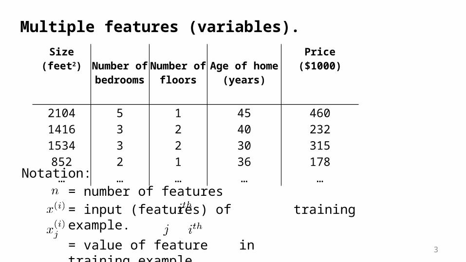
Multiple features (variables).

2

Size (feet2) Number of bedrooms

Number of floors

Age of home (years)

Price ($1000)

2104 5 1 45 4601416 3 2 40 2321534 3 2 30 315852 2 1 36 178… … … … …

Multiple features (variables).

Notation:= number of features= input (features) of training example.

= value of feature in training example.3

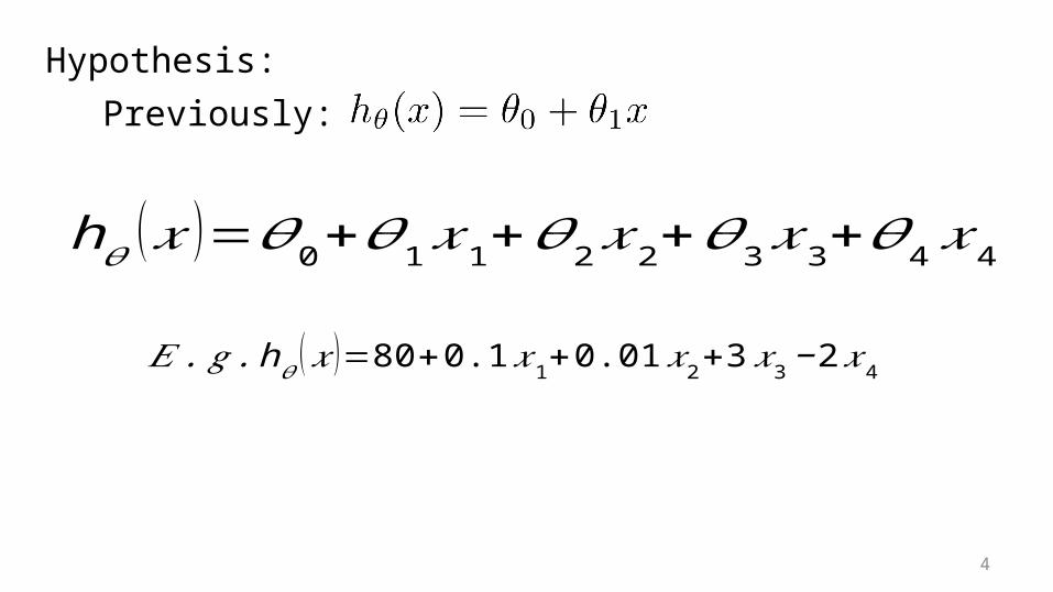
Hypothesis:Previously:

4

h𝜃 (𝑥 )=𝜃0+𝜃1𝑥1+𝜃2𝑥2+𝜃3𝑥3+𝜃4 𝑥4

𝐸 .𝑔 . h𝜃 (𝑥 )=80+0.1𝑥1+0.01𝑥2+3 𝑥3−2𝑥4

For convenience of notation, define .

Multivariate linear regression.5

Makes equation compact

Gradient descent for multiple variables

6

Hypothesis:

Cost function:

Parameters:

(simultaneously update for every )

Repeat

Gradient descent:

7

(simultaneously update )

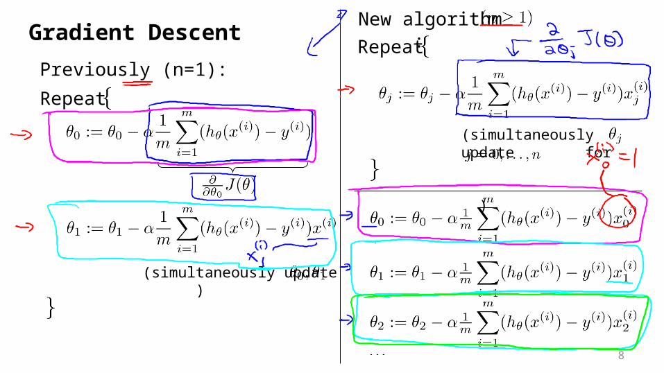
Gradient Descent

Repeat

Previously (n=1):

New algorithm :Repeat

(simultaneously update for )

8

Gradient descent in practice I: Feature Scaling

9

E.g. = size (0-2000 feet2)

= number of bedrooms (1-5)

Feature ScalingIdea: Make sure features are on a similar scale.

10

• Gradient Descent will have much harder time to find local minimum

• In terms of time i.e. iterations

11

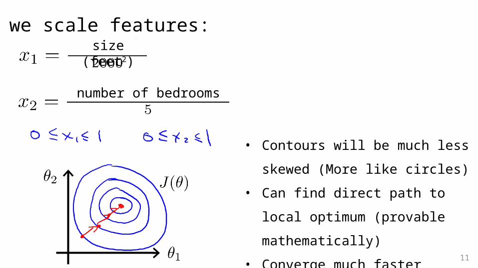
size (feet2)

number of bedrooms

If we scale features:

• Contours will be much less skewed

(More like circles)

• Can find direct path to local optimum

(provable mathematically)

• Converge much faster

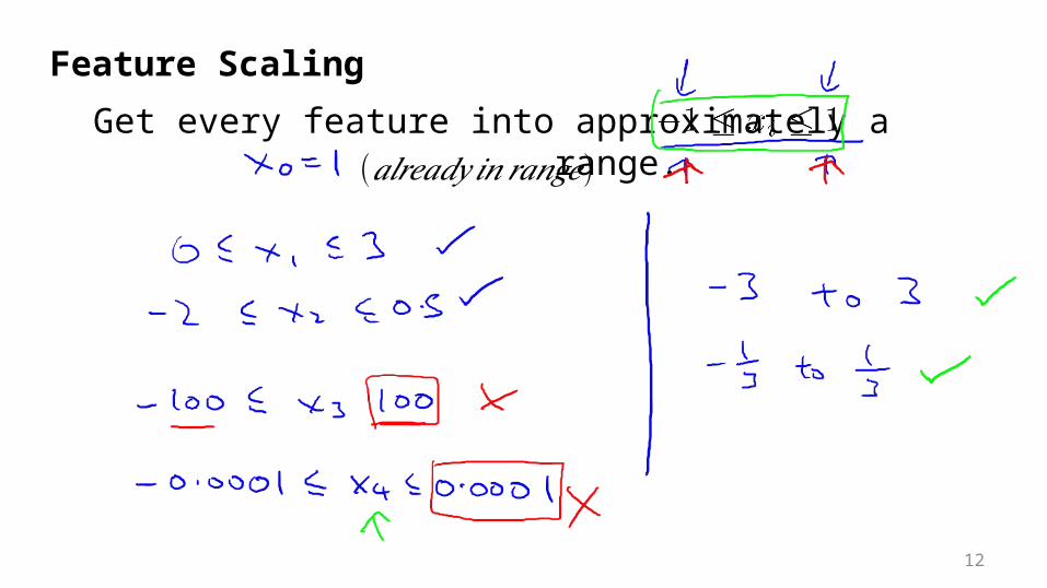
Feature Scaling

Get every feature into approximately a range.

12

(𝑎𝑙𝑟𝑒𝑎𝑑𝑦 𝑖𝑛𝑟𝑎𝑛𝑔𝑒)

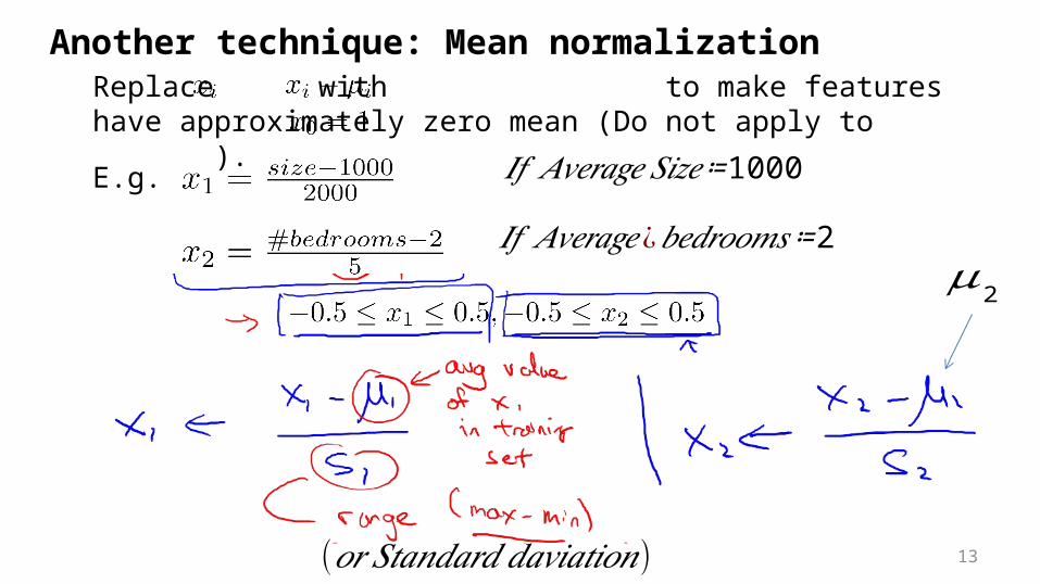
Replace with to make features have approximately zero mean (Do not apply to ).

Another technique: Mean normalization

E.g.

13

𝐼𝑓 𝐴𝑣𝑒𝑟𝑎𝑔𝑒𝑆𝑖𝑧𝑒≔1000

𝐼𝑓 𝐴𝑣𝑒𝑟𝑎𝑔𝑒 ¿𝑏𝑒𝑑𝑟𝑜𝑜𝑚𝑠≔ 2𝜇2

(𝑜𝑟 𝑆𝑡𝑎𝑛𝑑𝑎𝑟𝑑 𝑑𝑎𝑣𝑖𝑎𝑡𝑖𝑜𝑛)

14

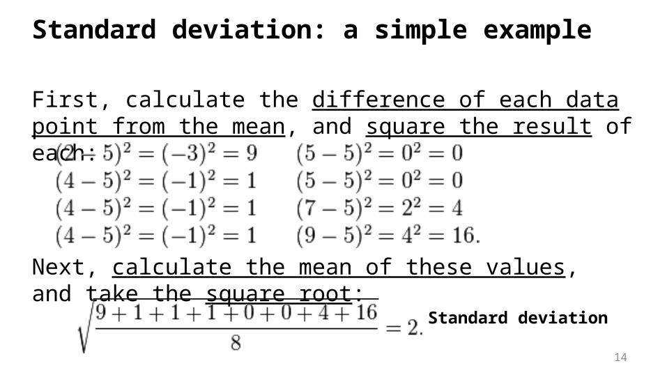
Standard deviation: a simple example First, calculate the difference of each data point from the mean, and square the result of each:

Next, calculate the mean of these values, and take the square root:

Standard deviation

Point to remember:• Feature Scaling and Mean normalization are

just approximations– So they do not have to be exact

• Our objective is to run Gradient Descent faster

15

Gradient descent in practice II: Learning rate

16

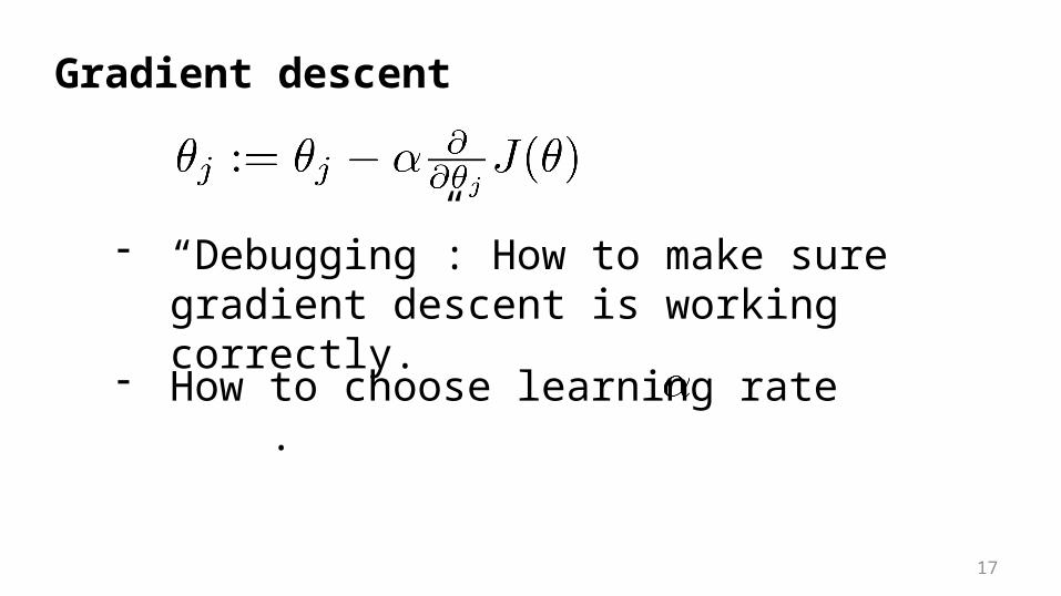
Gradient descent

- “Debugging”: How to make sure gradient descent is working correctly.

- How to choose learning rate .

17

Example automatic convergence test:

Declare convergence if decreases by less than in one iteration.

0 100 200 300 400

No. of iterations

Making sure gradient descent is working correctly.

18

• Plot vs. no of iterations • (i.e. plotting J(θ) over the course of gradient descent

• If gradient descent is working then J(θ) should decrease after every iteration

19

0 100 200 300 400

No. of iterations

• Number of iterations varies a lot:• 30 iterations• 3,000 iterations• 3,000,000 iterations

• Very hard to tell in advance how many iterations will be needed

• Can often make a guess based a plot like this after the first 100 or so iterations

Making sure gradient descent is working correctly.

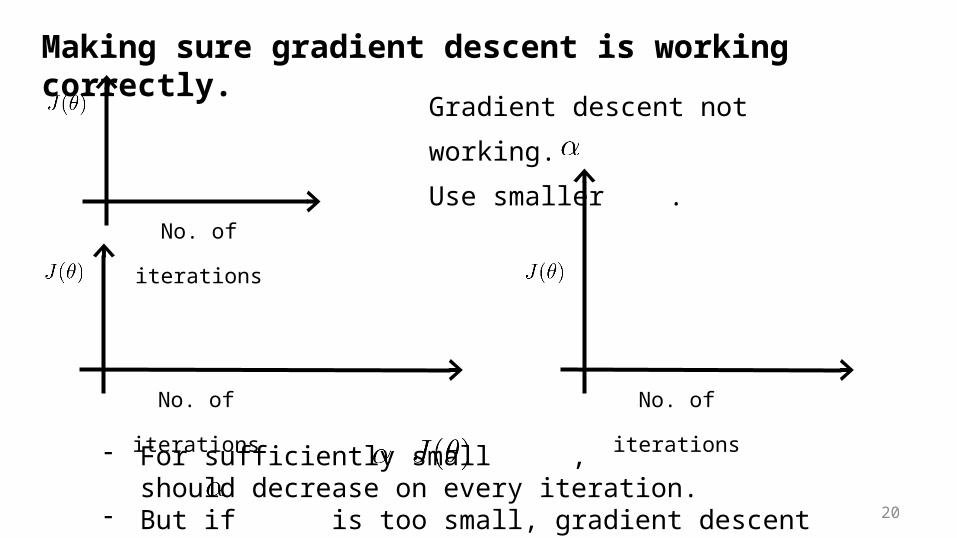
Making sure gradient descent is working correctly.

Gradient descent not working.

Use smaller .

No. of iterations

No. of iterations No. of iterations

- For sufficiently small , should decrease on every iteration.- But if is too small, gradient descent can be slow to converge.

20

Summary:- If is too small: slow convergence.- If is too large: may not decrease on

every iteration; may not converge.- For debugging you need to plot

To choose , try

21

Features and polynomial regression

22

Creating new features

Housing prices prediction

23

You don't have to use just two featuresMight decide that an important feature is the land area

Because, area is a better indicator

So, create a new feature:

Often, by defining new features you may get a better model

Polynomial regression

24

May fit the data bettere.g. a quadratic function • But may not fit the data so well• So instead must use a cubic

function

Polynomial regression

Price(y)

Size (x)

25

Choice of features

Price(y)

Size (x)

26

size ^(1/something) - i.e. square root, cubed root etc.

27

• Feature scaling becomes even more important here

• Later in class, we’ll look at developing an algorithm to chose the best features

Normal equation

28

For some linear regression problems, normal equation provides a better solution

Gradient Descent

Normal equation: Method to solve for analytically.Computing all in one go (in one step).

29

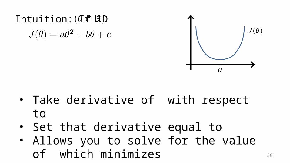
Intuition: If 1D

30

• Take derivative of with respect to • Set that derivative equal to • Allows you to solve for the value of which

minimizes

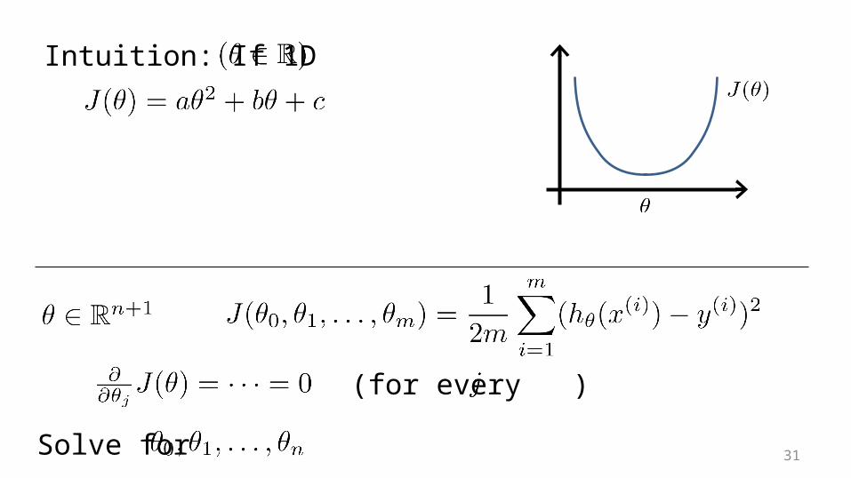
Intuition: If 1D

Solve for

(for every )

31

Size (feet2) Number of bedrooms

Number of floors

Age of home (years)

Price ($1000)

1 2104 5 1 45 4601 1416 3 2 40 2321 1534 3 2 30 3151 852 2 1 36 178

Size (feet2) Number of bedrooms

Number of floors

Age of home (years)

Price ($1000)

2104 5 1 45 4601416 3 2 40 2321534 3 2 30 315852 2 1 36 178

Examples:

32

34

is inverse of matrix .

Octave: pinv(X’*X)*X’*y

35

No Need of feature scaling

training examples, features.Gradient Descent Normal Equation

• No need to choose .• Don’t need to iterate.

• Need to choose . • Needs many iterations.• Works well even

when is large.• Need to compute

• Slow if is very large.

36

Normal equation and non-invertibility

37

Normal equation:- What if is non-invertible? (singular/

degenerate)- This should be quite a rare problem

- Octave:- Octave can invert matrices using

pinv()- This gets the right value even if (XT X)

is non-invertible

pinv(X’*X)*X’*y

38

What does it mean for (XT X) to be non-invertibleNormally two common causes:

• Redundant features (linearly dependent).E.g. size in feet2

size in m2

• Too many features (e.g. ).- Delete some features, or use regularization.

39

End

40