04a lecture riskpreferencesmarkus/teaching/fin501/04lecture.pdf · fin 501: asset pricing lecture...
TRANSCRIPT

Fin 501: Asset Pricing
Lecture Lecture 04: 04: Risk Preferences and Risk Preferences and Expected Expected Utility TheoryUtility Theory
• Prof. Markus K. Brunnermeier
Slide 04Slide 04--11

Fin 501: Asset Pricing
O iO i Ri k P fRi k P fOverview: Overview: Risk PreferencesRisk Preferences
1.1. StateState--byby--state dominancestate dominance2.2. Stochastic dominanceStochastic dominance [DD4][DD4]
3.3. vNMvNM expected utility theoryexpected utility theorya)a) IntuitionIntuition [L4][L4]
b)b) A i ti f d tiA i ti f d tib)b) Axiomatic foundationsAxiomatic foundations [DD3][DD3]
4.4. Risk aversion coefficients and Risk aversion coefficients and pportfolio choice ortfolio choice [DD5,L4][DD5,L4]
55 Prudence coefficient and precautionary savingsPrudence coefficient and precautionary savings [DD5][DD5]5.5. Prudence coefficient and precautionary savings Prudence coefficient and precautionary savings [DD5][DD5]
6.6. MeanMean--variance preferencesvariance preferences [L4.6][L4.6]
Slide 04Slide 04--22

Fin 501: Asset Pricing
St tSt t bb t t D it t D iStateState--byby--state Dominancestate Dominance- State-by-state dominance incomplete rankingy p g- « riskier »
Table 2.1 Asset Payoffs ($)
t = 0 t = 1 Cost at t=0 Value at t=1
½π1 = π2 = ½ s = 1 s = 2 investment 1 i t t 2
- 1000 1000
1050 500
1200 1600investment 2
investment 3 - 1000- 1000
500 1050
16001600
Slide 04Slide 04--33
- investment 3 state by state dominates 1.

Fin 501: Asset Pricing
St tSt t bb t t D i ( td )t t D i ( td )StateState--byby--state Dominance (ctd.)state Dominance (ctd.)
Table 2.2 State Contingent ROR (r )
St t C ti t ROR ( ) State Contingent ROR (r ) s = 1 s = 2 Er σ Investment 1 5% 20% 12.5% 7.5% Investment 2Investment 3
-50% 5%
60%60%
5% 32.5%
55% 27.5%
- Investment 1 mean-variance dominates 2- BUT investment 3 does not m-v dominate 1!
Slide 04Slide 04--44

Fin 501: Asset Pricing
St tSt t bb t t D i ( td )t t D i ( td )StateState--byby--state Dominance (ctd.)state Dominance (ctd.)Table 2.3 State Contingent Rates of Return
State Contingent Rates of Return s = 1 s = 2investment 4 investment 5
3% 3%
5% 8%
π1 = π2 = ½ E[r4] = 4%; σ4 = 1% E[r ] = 5 5%; σ = 2 5%E[r5] = 5.5%; σ5 = 2.5%
- What is the trade-off between risk and expected return?I 4 h hi h Sh i (E[ ] f)/ h i 5
Slide 04Slide 04--55
- Investment 4 has a higher Sharpe ratio (E[r]-rf)/σ than investment 5for rf = 0.

Fin 501: Asset Pricing
O iO i Ri k P fRi k P fOverview: Overview: Risk PreferencesRisk Preferences
1.1. StateState--byby--state dominancestate dominance2.2. Stochastic dominanceStochastic dominance [DD4][DD4]
3.3. vNMvNM expected utility theoryexpected utility theorya)a) IntuitionIntuition [L4][L4]
b)b) A i ti f d tiA i ti f d tib)b) Axiomatic foundationsAxiomatic foundations [DD3][DD3]
c)c) Risk aversion coefficientsRisk aversion coefficients [DD4,L4][DD4,L4]
44 Risk aversion coefficients andRisk aversion coefficients and pportfolio choiceortfolio choice [DD5 L4][DD5 L4]4.4. Risk aversion coefficients and Risk aversion coefficients and pportfolio choice ortfolio choice [DD5,L4][DD5,L4]
5.5. Prudence coefficient and precautionary savings Prudence coefficient and precautionary savings [DD5][DD5]
6.6. MeanMean--variance preferencesvariance preferences [L4.6][L4.6]
Slide 04Slide 04--66
6.6. MeanMean variance preferencesvariance preferences [L4.6][L4.6]

Fin 501: Asset Pricing
St h ti D iSt h ti D iStochastic DominanceStochastic DominanceStill incomplete orderingp g
“More complete” than state-by-state orderingState-by-state dominance ⇒ stochastic dominanceRisk preference not needed for ranking!
independently of the specific trade-offs (between return, risk and other characteristics of probability distributions) represented by an agent'scharacteristics of probability distributions) represented by an agent s utility function. (“risk-preference-free”)
Next Section: Complete preference ordering and utility representations
H k P id l hi h b k d
Slide 04Slide 04--77
Homework: Provide an example which can be ranked according to FSD , but not according to state dominance.

Fin 501: Asset Pricing Table 3-1 Sample Investment Alternatives
States of nature 1 2 3Payoffs 10 100 2000Proba Z1 .4 .6 0Proba Z2 .4 .4 .2
EZ1 = 64, 1zσ = 441z
EZ2 = 444, 2zσ = 779
1 0F1
obabilityPr
0 7
0.8
0.9
1.0
F2
0.4
0.5
0.6
0.7
F1 and F 2
0 1
0.4
0.2
0.3
Slide 04Slide 04--880 10 100 2000
0.1
Payoff

Fin 501: Asset Pricing
Fi t O d St h ti D iFi t O d St h ti D iDefinition 3 1 : Let F (x) and F (x) respectively
First Order Stochastic DominanceFirst Order Stochastic DominanceDefinition 3.1 : Let FA(x) and FB(x) , respectively, represent the cumulative distribution functions of two random variables (cash payoffs) that, without loss of ( p y ff ) , fgenerality assume values in the interval [a,b]. We say that FA(x) first order stochastically dominates (FSD)FB(x) if and only if for all x ∈ [a,b]
FA(x) ≤ FB(x)
H k P id l hi h b k d
Slide 04Slide 04--99
Homework: Provide an example which can be ranked according to FSD , but not according to state dominance.

Fin 501: Asset Pricing
Fi t O d St h ti D iFi t O d St h ti D i1
First Order Stochastic DominanceFirst Order Stochastic Dominance
0.7
0.8
0.9
1
FA
FB
0.4
0.5
0.6
0
0.1
0.2
0.3
X
0
0 1 2 3 4 5 6 7 8 9 10 11 12 13 14
Slide 04Slide 04--1010
Fin 501: Asset Pricing
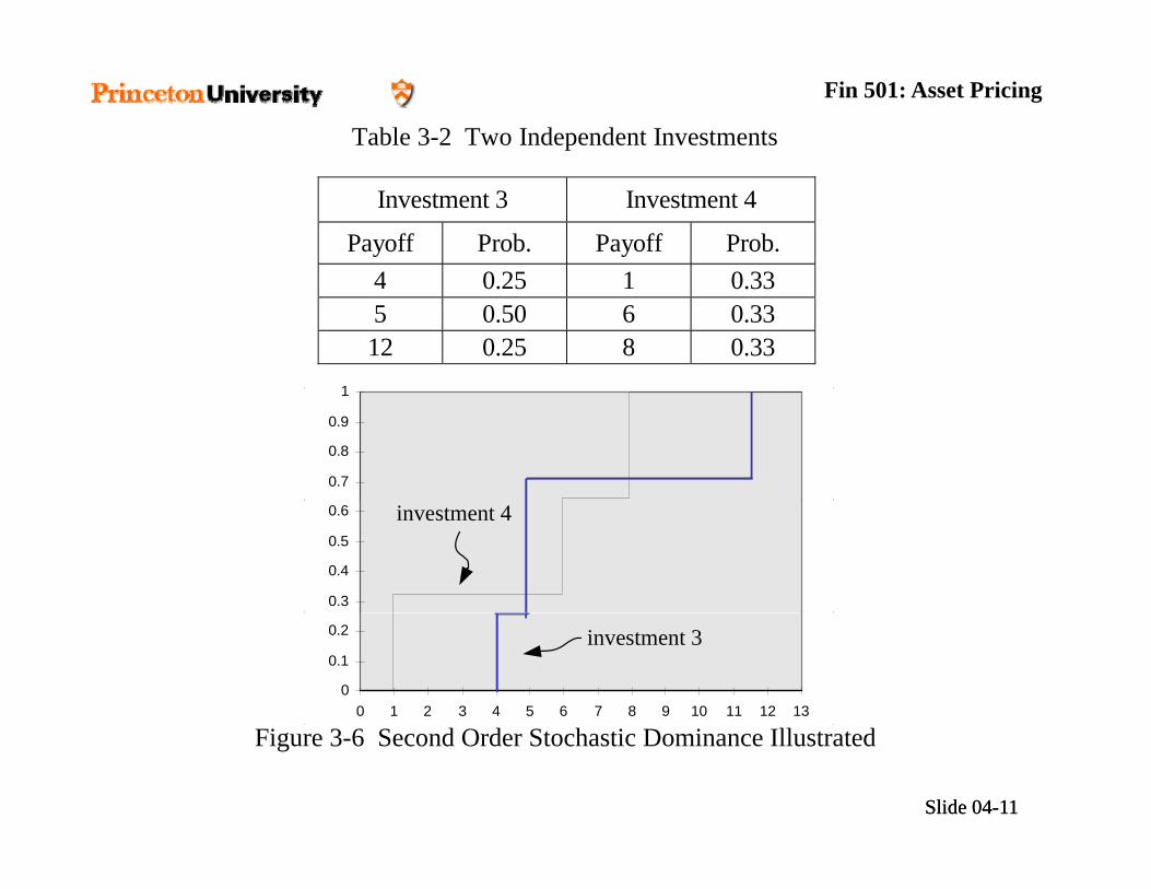
Table 3-2 Two Independent Investments
Investment 3 Investment 4
Payoff Prob. Payoff Prob.4 0 25 1 0 33
1
4 0.25 1 0.335 0.50 6 0.3312 0.25 8 0.33
0.7
0.8
0.9
1
0.3
0.4
0.5
0.6 investment 4
0
0.1
0.2
0 1 2 3 4 5 6 7 8 9 10 11 12 13
investment 3
Slide 04Slide 04--1111
Figure 3-6 Second Order Stochastic Dominance Illustrated

Fin 501: Asset Pricing
S d O d St h ti D iS d O d St h ti D iDefinition 3 2: Let be two)x~(F )x~(F
Second Order Stochastic DominanceSecond Order Stochastic DominanceDefinition 3.2: Let , , be two cumulative probability distribution for random payoffs in We say that
)x(FA )x(FB
[ ]b,a )x~(FArandom payoffs in . We say that second order stochastically dominates(SSD) if and only if for any x :
[ ]b,a )x(FA
)x~(FB(SSD) if and only if for any x :)x(FB
[ ] 0dt(t)F(t)Fx
≥∫
(with strict inequality for some meaningful
[ ] 0dt (t)F-(t)F AB-
≥∫∞
Slide 04Slide 04--1212
interval of values of t).

Fin 501: Asset Pricing
Mean Preserving SpreadMean Preserving SpreadxB = xA + z (3.8)B A ( )
where z is independent of xA and has zero mean
( )f xAfor normal distributions
( )f xB( )
~,x Payoff( ) ( )∫ ∫f d f d
Slide 04Slide 04--1313
( ) ( )μ = =∫ ∫x f x dx x f x dxA B
Figure 3-7 Mean Preserving Spread

Fin 501: Asset Pricing
Mean Preserving Spread & SSDMean Preserving Spread & SSD
Theorem 3.4 : Let (•) and (•) be two distribution functions defined on the same state space with identical
AF BF
means. Then the follow statements are equivalent :
SSDis a mean preserving spread of
)x~(FA )x~(FB
)x~(FB )x~(FAis a mean p ese ving sp ead ofin the sense of Equation (3.8) above.
)(B )(A
Slide 04Slide 04--1414

Fin 501: Asset Pricing
O iO i Ri k P fRi k P fOverview: Overview: Risk PreferencesRisk Preferences
1.1. StateState--byby--state dominancestate dominance2.2. Stochastic dominanceStochastic dominance [DD4][DD4]
3.3. vNMvNM expected utility theoryexpected utility theorya)a) IntuitionIntuition [L4][L4]
b)b) A i ti f d tiA i ti f d tib)b) Axiomatic foundationsAxiomatic foundations [DD3][DD3]
4.4. Risk aversion coefficients and Risk aversion coefficients and pportfolio choice ortfolio choice [DD4,5,L4][DD4,5,L4]
55 Prudence coefficient and precautionary savingsPrudence coefficient and precautionary savings [DD5][DD5]5.5. Prudence coefficient and precautionary savings Prudence coefficient and precautionary savings [DD5][DD5]
6.6. MeanMean--variance preferencesvariance preferences [L4.6][L4.6]
Slide 04Slide 04--1515

Fin 501: Asset Pricing
A H th ti l G blA H th ti l G blA Hypothetical GambleA Hypothetical GambleSuppose someone offers you this gamble:Suppose someone offers you this gamble:
"I have a fair coin here. I'll flip it, and if it's tail I pay you $1 and the gamble is over. If it's head, I'll flip again. If it's tail then, I pay you $2, if not I'll flip again. With every round, I double the amount I will pay to you if it's tail "you if it s tail.
Sounds like a good deal. After all, you can't loose. So here's the question:So here s the question:
How much are you willing to pay to take this gamble?
Slide 04Slide 04--1616
g

Fin 501: Asset Pricing
P l 1P l 1 E t d V lE t d V lProposal 1: Proposal 1: Expected ValueExpected Value
With probability 1/2 you get $1.With probability 1/4 you get $2
( ) 0121 2 times
( ) 121 2 times With probability 1/4 you get $2.With probability 1/8 you get $4.
( )2 2 times
( ) 2321 2 times
etc.The expected payoff is the sum of these payoffs weighted with their probabilities
∑∞
−⋅⎟⎠⎞
⎜⎝⎛ 1221 t
t
∑∞
=1 21
t∞=
payoffs, weighted with their probabilities, so
Slide 04Slide 04--1717
{∑
= ⎠⎝1 2t
payoffyprobabilit321 =1 2t

Fin 501: Asset Pricing
An Infinitely Valuable Gamble?An Infinitely Valuable Gamble?An Infinitely Valuable Gamble?An Infinitely Valuable Gamble?You should pay everything you own and 0.5
probability
everything you own and more to purchase the right to take this gamble! 0.3
0.4
to take this gamble!
Yet, in practice, no one is prepared to pay such a 0.1
0.2
prepared to pay such a high price. Why?
E th h th t d
00 20 40 60 $
Even though the expected payoff is infinite, the distribution of payoffs is
With 93% probability we get $8 or less, with
b biliSlide 04Slide 04--1818
distribution of payoffs is not attractive…
99% probability we get $64 or less.

Fin 501: Asset Pricing
What Sho ld We Do?What Sho ld We Do?What Should We Do?What Should We Do?How can we decide in a rational fashion about such gambles (or investments)?Proposal 2: Bernoulli suggests that large gains should be weighted less. He suggests to use the natural logarithm. [Cremer - another great mathematician of the time - suggests the square root ]square root.]
∑∞
−⋅⎟⎠⎞
⎜⎝⎛ 1)2ln(21 t
t
∞<==gamble of
utility expected)2ln(
{∑
= ⎠⎝1
2t
payoffofutilityyprobabilit43421
gamble of
Bernoulli would have paid at most eln(2) = $2 to
Slide 04Slide 04--1919
Bernoulli would have paid at most e $2 to participate in this gamble.

Fin 501: Asset Pricing
Ri kRi k A i d C itA i d C itRiskRisk--Aversion and ConcavityAversion and Concavityu(x)
The shape of the von Neumann Morgenstern (NM) utility function contains a lot
( )
utility function contains a lot of information.Consider a fifty-fifty lottery
u(x1)
with final wealth of x0 or x1E{u(x)}
u(x0)
Slide 04Slide 04--2020xx0 x1E[x]

Fin 501: Asset Pricing
Ri kRi k i d iti d itRiskRisk--aversion and concavityaversion and concavityu(x)
Risk-aversion means that the certainty equivalent is smaller than the expected prize
( )
than the expected prize.We conclude that a risk-averse vNMutility function
u(x1)
u(E[x])
E[u(x)]
utility function must be concave.
u(x0)
Slide 04Slide 04--2121xx0 x1E[x]
u-1(E[u(x)])

Fin 501: Asset Pricing
J ’ I litJ ’ I litTheorem 3 1 (Jensen’s Inequality):
Jensen’s InequalityJensen’s InequalityTheorem 3.1 (Jensen s Inequality):
Let g( ) be a concave function on the interval [a,b], and be a random variable such that[ ]
Prob (x ∈[a,b]) =1Suppose the expectations E(x) and E[g(x)] exist; then
[ ] [ ])~()~( xEgxgE ≤
Furthermore, if g(•) is strictly concave, then the inequality is strict.
Slide 04Slide 04--2222

Fin 501: Asset Pricing
R t ti f P fR t ti f P fRepresentation of PreferencesRepresentation of Preferences
A preference ordering is (i) complete, (ii) transitive, (iii) continuous and [(iv) relatively stable] can be represented by a utility function, i.e.
(c c c ) Â (c’ c’ c’ )(c0,c1,…,cS) Â (c 0,c 1,…,c S) ⇔ U(c0,c1,…,cS) > U(c’0,c’1,…,c’S)
(preference ordering over lotteries –(S+1)-dimensional space)
Slide 04Slide 04--2323
(S ) p )

Fin 501: Asset Pricing
P f P b Di t ib tiP f P b Di t ib tiPreferences over Prob. DistributionsPreferences over Prob. Distributions
Consider c0 fixed, c1 is a random variablePreference ordering over probability distributionsPreference ordering over probability distributionsLet
P b t f b bilit di t ib ti ith fi itP be a set of probability distributions with a finite support over a set X,  a (strict) preference ordering over P and a (strict) preference ordering over P, andDefine % by p % q if q ¨ p
Slide 04Slide 04--2424

Fin 501: Asset Pricing
S states of the worldS states of the worldSet of all possible lotteries
Space with S dimensionsSpace with S dimensions
C i lif th tilit t ti fCan we simplify the utility representation of preferences over lotteries?S ith di i iSpace with one dimension – incomeWe need to assume further axioms
Slide 04Slide 04--2525

Fin 501: Asset Pricing
E t d Utilit ThE t d Utilit ThExpected Utility TheoryExpected Utility Theory
A binary relation that satisfies the following three axioms if and only if there exists a function yu(•) such that
p  q ⇔ ∑ u(c) p(c) > ∑ u(c) q(c)
i.e. preferences correspond to expected utility.
Slide 04Slide 04--2626

Fin 501: Asset Pricing
NM E t d Utilit ThNM E t d Utilit ThvNM Expected Utility TheoryvNM Expected Utility TheoryAxiom 1 (Completeness and Transitivity):( p y)
Agents have preference relation over P (repeated)Axiom 2 (Substitution/Independence)Axiom 2 (Substitution/Independence)
For all lotteries p,q,r ∈ P and α ∈ (0,1], p < q iff α p + (1-α) r < α q + (1-α) r (see next slide)p < q p ( ) < q ( ) ( )
Axiom 3 (Archimedian/Continuity)For all lotteries p q r ∈ P if p  q  r then thereFor all lotteries p,q,r ∈ P, if p  q  r, then there exists a α , β ∈ (0,1) such that α p + (1- α) r  q  β p + (1 - β) r.
Slide 04Slide 04--2727
α p ( α)  q  β p ( β) .Problem: p you get $100 for sure, q you get $ 10 for sure, r you are killed

Fin 501: Asset Pricing
I d d A iI d d A iIndependence AxiomIndependence Axiom
Independence of irrelevant alternatives:
p < q ⇔π π
p q
<p < q
r r
<
Slide 04Slide 04--2828

Fin 501: Asset Pricing
Allais ParadoxAllais Paradox ––Allais Paradox Allais Paradox Violation of Independence AxiomViolation of Independence Axiom
10’ 15’9%10%
0 0
≺
Slide 04Slide 04--2929

Fin 501: Asset Pricing
Allais ParadoxAllais Paradox ––Allais Paradox Allais Paradox Violation of Independence AxiomViolation of Independence Axiom
10’ 15’9%10%
0 0
≺
10’ 15’90%100%
Â0 0
Â
Slide 04Slide 04--3030

Fin 501: Asset Pricing
Allais ParadoxAllais Paradox ––Allais Paradox Allais Paradox Violation of Independence AxiomViolation of Independence Axiom
10’ 15’9%10%
0 0
≺
10’ 15’90%100%
Â10%0 0
Â10% 10%
Slide 04Slide 04--3131
0 0

Fin 501: Asset Pricing
NM EU ThNM EU ThvNM EU TheoremvNM EU Theorem
A binary relation that satisfies the axioms 1-3 if and only if there exists a function u(•) such that y ( )
p  q ⇔ ∑ u(c) p(c) > ∑ u(c) q(c)p q ( ) p( ) ( ) q( )
i.e. preferences correspond to expected utility.p p p y
Slide 04Slide 04--3232

Fin 501: Asset Pricing
E t d Utilit ThE t d Utilit ThExpected Utility TheoryExpected Utility TheoryU(Y)U(Y)
)ZY(U 20 +
))Z~(EY(U +~
))Z(EY(U 0 +)ZY(EU 0 +
)ZY(U 10 +
Y~ ~
Π)Z~(CE
0Y 10 ZY + )ZY(CE 0 + )Z(EY0 + 20 ZY +
Slide 04Slide 04--3333

Fin 501: Asset Pricing
Expected Utility & Stochastic DominanceExpected Utility & Stochastic Dominance
Theorem 3. 2 : Let , , be two cumulative b bilit di t ib ti f d ff
)x~(FA )x~(FB
[ ]bax~ ∈probability distribution for random payoffs . Then FSD if and only if for all non decreasing utility functions U(•)
[ ]b,ax ∈)x~(FA )x~(FB
for all non decreasing utility functions U( ). )x~U(E)x~U(E BA ≥
Slide 04Slide 04--3434

Fin 501: Asset Pricing
Expected Utility & Stochastic DominanceExpected Utility & Stochastic Dominance
Theorem 3. 3 : Let , , be two cumulative probability distribution
)x~(FA )x~(FB
p yfor random payoffs defined on . Then, SSD if and only iff ll d d
x~ [ ]b,a)x~(FA )x~(FB )x~U(E)x~U(E BA ≥
for all non decreasing and concave U.
Slide 04Slide 04--3535

Fin 501: Asset Pricing
S bj ti EU ThS bj ti EU ThDigression:Digression: Subjective EU TheorySubjective EU Theory
Derive perceived probability from preferences!Set S of prizes/consequencesSet S of prizes/consequencesSet Z of states Set of functions f(s) ∈ Z called acts (consumption plans)Set of functions f(s) ∈ Z, called acts (consumption plans)
Seven SAVAGE AxiomsG b d f thiGoes beyond scope of this course.
Slide 04Slide 04--3636

Fin 501: Asset Pricing
Ell b P dEll b P dDigression:Digression: Ellsberg ParadoxEllsberg Paradox
10 balls in an urn Lottery 1: win $100 if you draw a red ballL tt 2 i $100 if d bl b llLottery 2: win $100 if you draw a blue ball
Uncertainty: Probability distribution is not knownRisk: Probability distribution is known
(5 balls are red, 5 balls are blue)
Individuals are “uncertainty/ambiguity averse”
Slide 04Slide 04--3737
(non-additive probability approach)

Fin 501: Asset Pricing
P t ThP t ThDigression:Digression: Prospect TheoryProspect TheoryValue function (over gains and losses)( g )
Overweight low probability eventsExperimental evidence
Slide 04Slide 04--3838
Experimental evidence

Fin 501: Asset Pricing
I diffI diffIndifference curvesIndifference curvesx2
Any point in this plane is 2 this plane is a particular lottery.
Where is the set of risk-f free lotteries?
If x x
x1
If x1=x2, then the lottery 45°
Slide 04Slide 04--3939
x1 contains no risk.

Fin 501: Asset Pricing
I diffI diffIndifference curvesIndifference curvesx2
Where is the set of lotteries 2 set of lotteries with expected prize E[L]=z?π
It's a straight line, and the slope is given by the
z
x1
given by the relative probabilities of the two
45°
Slide 04Slide 04--4040
x1 of the two states.
z
Fin 501: Asset Pricing
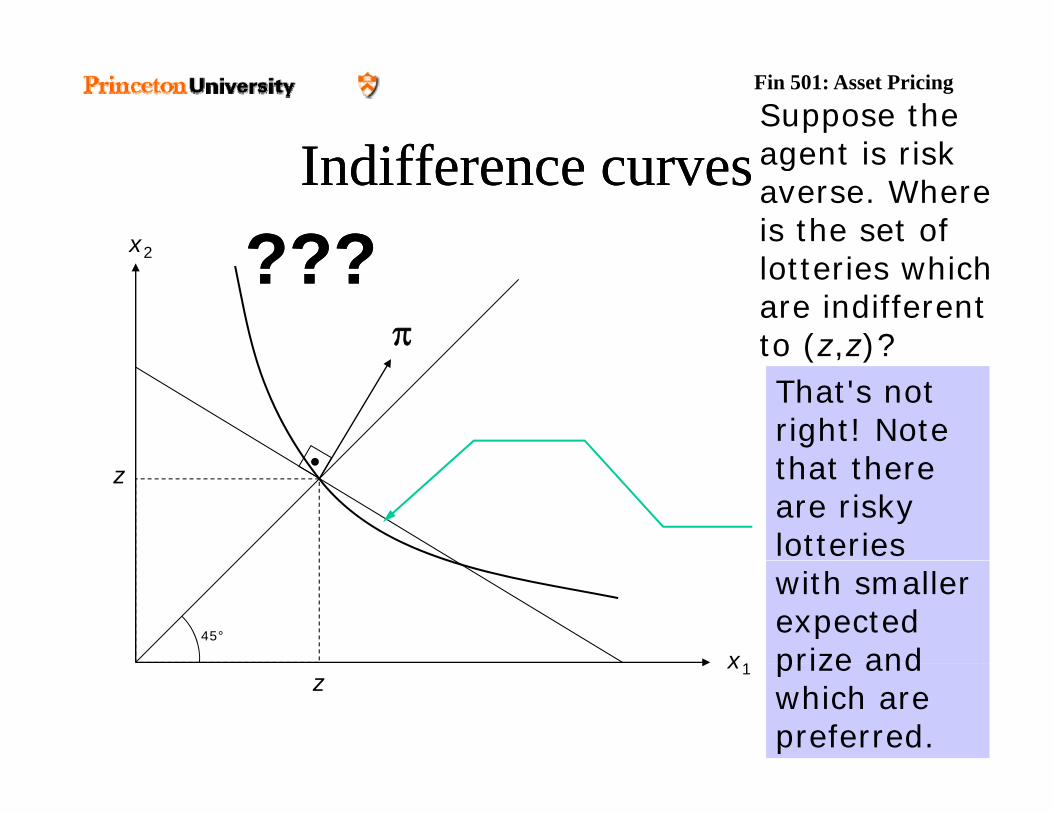
I diffI diffSuppose the agent is risk Indifference curvesIndifference curves
x2
agent is risk averse. Where is the set of ??????2lotteries which are indifferent to (z,z)?π
??????to (z,z)?That's not right! Note th t th that there are risky lotteries
z
x1
with smaller expected prize and
45°
Slide 04Slide 04--4141
x1 prize and which are preferred.
z

Fin 501: Asset Pricing
I diffI diffIndifference curvesIndifference curvesx2 So the 2 So the
indifference curve must be πtangent to the iso-expected-prize line.prize line.
This is a direct implication of
z
x1
prisk-aversion alone.
45°
Slide 04Slide 04--4242
x1z

Fin 501: Asset Pricing
I diffI diffIndifference curvesIndifference curvesx2 But risk2
π
But risk-aversion does not imply convexity.
This d ffz indifference
curve is also compatible
x1
45°
pwith risk-aversion.
Slide 04Slide 04--4343
x1z

Fin 501: Asset Pricing
I diffI diffIndifference curvesIndifference curvesx2 The tangency 2
∇ V(z,z)The tangency implies that the gradient
π of V at the point (z,z) is collinear to π.
zcollinear to π.
Formally,∇ V(z,z) = λπ,
x1
45°
∇ V(z,z) λπ, for some λ>0.
Slide 04Slide 04--4444
x1z

Fin 501: Asset Pricing
C i E i l d Ri k P iC i E i l d Ri k P iCertainty Equivalent and Risk PremiumCertainty Equivalent and Risk Premium
(3.6) EU(Y + ) = U(Y + CE(Y, ))Z~ Z~
(3.7) = U(Y +E - Π(Y, )) Z~ Z~
Slide 04Slide 04--4545

Fin 501: Asset Pricing
C i E i l d Ri k P iC i E i l d Ri k P iU(Y)
Certainty Equivalent and Risk PremiumCertainty Equivalent and Risk Premium
~
)ZY(U 20 +
))Z~(EY(U 0 +)ZY(EU 0 +0
)ZY(U 10 +
Π)Z~(CE
Y~ ~
0Y 10 ZY + )ZY(CE 0 + )Z(EY0 + 20 ZY +
Figure 3-3 Certainty Equivalent and Risk Premium: An Illustration
Slide 04Slide 04--4646
g y q

Fin 501: Asset Pricing
O iO i Ri k P fRi k P fOverview: Overview: Risk PreferencesRisk Preferences
1.1. StateState--byby--state dominancestate dominance2.2. Stochastic dominanceStochastic dominance [DD4][DD4]
3.3. vNMvNM expected utility theoryexpected utility theorya)a) IntuitionIntuition [L4][L4]
b)b) A i ti f d tiA i ti f d tib)b) Axiomatic foundationsAxiomatic foundations [DD3][DD3]
4.4. Risk aversion coefficients and Risk aversion coefficients and pportfolio choice ortfolio choice [DD4,5,L4][DD4,5,L4]
55 Prudence coefficient and precautionary savingsPrudence coefficient and precautionary savings [DD5][DD5]5.5. Prudence coefficient and precautionary savings Prudence coefficient and precautionary savings [DD5][DD5]
6.6. MeanMean--variance preferencesvariance preferences [L4.6][L4.6]
Slide 04Slide 04--4747

Fin 501: Asset Pricing
M i Ri k iM i Ri k iU(W)
li
Measuring Risk aversionMeasuring Risk aversiontangent lines
U(Y+h)
U[0.5(Y+h)+0.5(Y-h)]
0.5U(Y+h)+0.5U(Y-h)
U(Y-h)
WY-h Y Y+h
Slide 04Slide 04--4848
Figure 3-1 A Strictly Concave Utility Function

Fin 501: Asset Pricing
AA P tt f i k iP tt f i k iArrowArrow--Pratt measures of risk aversion Pratt measures of risk aversion and their interpretationsand their interpretations
absolute risk aversion (Y)(Y) U"absolute risk aversion (Y)R(Y) U'( ) -= A≡
relative risk aversion (Y) R (Y)U'
(Y) U"Y - = R≡
risk tolerance =
( )
Slide 04Slide 04--4949

Fin 501: Asset Pricing
Ab l t i k i ffi i tAb l t i k i ffi i tAbsolute risk aversion coefficientAbsolute risk aversion coefficient
YY+hπ
Y-h1−π
Slide 04Slide 04--5050

Fin 501: Asset Pricing
R l ti i k i ffi i tR l ti i k i ffi i tRelative risk aversion coefficientRelative risk aversion coefficient
YY(1+θ)π
Y(1-θ)1−π
Slide 04Slide 04--5151
Homework: Derive this result.

Fin 501: Asset Pricing
CARA d CRRACARA d CRRA tilit f titilit f tiCARA and CRRACARA and CRRA--utility functionsutility functions
Constant Absolute RA utility function
C R l i RA ili f iConstant Relative RA utility function
Slide 04Slide 04--5252

Fin 501: Asset Pricing
’ l f l i i k A i’ l f l i i k A iInvestorInvestor ’s Level of Relative Risk Aversion’s Level of Relative Risk Aversion
γ+
γ+
γ+ γ−γ−γ−
- 1)100,000Y( +
- 1)50,000Y( =
-1)CEY( 1
21 1
21 1
γ = 0 CE = 75,000 (risk neutrality)γ = 1 CE = 70,711γ 2 CE 66 246γ = 2 CE = 66,246γ = 5 CE = 58,566γ = 10 CE = 53,991
Y=0
γ = 20 CE = 51,858γ = 30 CE = 51,209
Slide 04Slide 04--5353
Y=100,000 γ = 5 CE = 66,530

Fin 501: Asset Pricing
Ri k i d P tf li All tiRi k i d P tf li All tiRisk aversion and Portfolio AllocationRisk aversion and Portfolio AllocationN i d i i ( i l 1)No savings decision (consumption occurs only at t=1)
Asset structureOne risk free bond with net return rf
One risky asset with random net return r (a =quantity of risky assets)
Slide 04Slide 04--5454

Fin 501: Asset Pricing
• Theorem 4.1: Assume U'( ) > 0, and U"( ) < 0 and let â ( ) , ( )denote the solution to above problem. Then
rr~E ifonly and if 0a f>>
. rr~E ifonly and if 0arr~E ifonly and if 0a
f
f
<<==
• Define . The FOC can then be written = 0 . By risk aversion (U''<0)
( ) ( ) ( )( ){ }ff0 rr~ar1YUEaW −++=( ) ( ) ( )( )( )[ ]fff0 rr~rr~ar1YUEaW −−++′=′
( ) ( ) ( )( )( )[ ]2~~1YUEW ′′′′By risk aversion (U''<0), < 0, that is, W'(a) is everywhere decreasing. It follows that â will be positive if and only if
( ) ( ) ( )( )( )[ ]2fff0 rr~rr~ar1YUEaW −−++′′=′′
( ) ( )( ) ( ) 0rr~Er1YU0W ff0 >−+′=′
(since then a will have to be increased from its value of 0 to achieve equality in the FOC). Since U' is always strictly positive this implies if and only if0a > ( ) 0rr~E > W’(a)
Slide 04Slide 04--5555
positive, this implies if and only if . The other assertion follows similarly.
0a > ( ) 0rrE f >−
a
W (a)
0

Fin 501: Asset Pricing
P tf li lth hP tf li lth hPortfolio as wealth changesPortfolio as wealth changes
• Theorem 4.4 (Arrow, 1971): Let be the solution to max-problem above; then:
(i)
(ii)
(iii) .
Slide 04Slide 04--5656
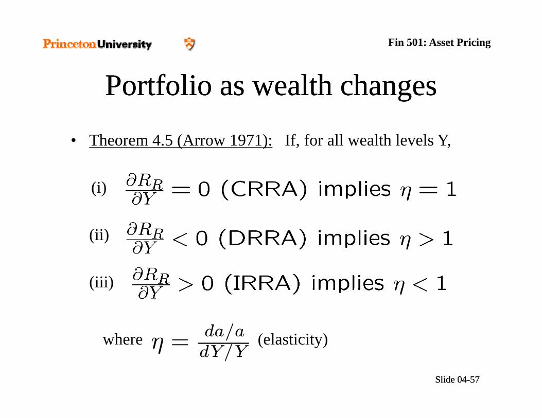
Fin 501: Asset Pricing
P tf li lth hP tf li lth hPortfolio as wealth changesPortfolio as wealth changes
• Theorem 4.5 (Arrow 1971): If, for all wealth levels Y,
(i)(i)
(ii)(ii)
(iii) ( )
where (elasticity)η = da/a
Slide 04Slide 04--5757
where (elasticity)η = dY/Y
Fin 501: Asset Pricing
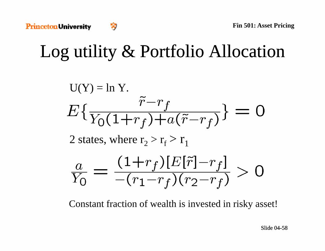
L tilit & P tf li All tiL tilit & P tf li All tiLog utility & Portfolio Allocation Log utility & Portfolio Allocation
U(Y) = ln Y.
2 states where r2 > rf > r12 states, where r2 > rf > r1
Constant fraction of wealth is invested in risky asset!
Slide 04Slide 04--5858
Constant fraction of wealth is invested in risky asset!

Fin 501: Asset Pricing
Portfolio of risky assets as wealth changesPortfolio of risky assets as wealth changesPortfolio of risky assets as wealth changesPortfolio of risky assets as wealth changesNow -- many risky assets
Theorem 4.6 (Cass and Stiglitz,1970). Let the vector
denote the amount optimally invested in the J risky assets if⎥⎤
⎢⎡ )Y(â 01 p y y
⎥⎥⎥⎥
⎦⎢⎢⎢⎢
⎣ )Y(â..
0Ja)Y(â 101
⎥⎥⎤
⎢⎢⎡
⎥⎥⎤
⎢⎢⎡
the wealth level is Y0.. Then
if d l if ith
)Y(f
a..
)Y(â..
0
J0J⎥⎥⎥
⎦⎢⎢⎢
⎣
=
⎥⎥⎥
⎦⎢⎢⎢
⎣if and only if either
(i) or(ii) .
Δκ+θ= )Y()Y('U 00
0Y0 e)Y('U ν−ξ=
Slide 04Slide 04--5959
In words, it is sufficient to offer a mutual fund.
Fin 501: Asset Pricing
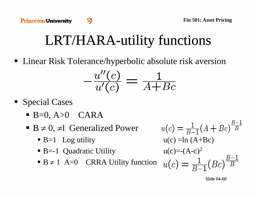
LRT/HARALRT/HARA tilit f titilit f tiLinear Risk Tolerance/hyperbolic absolute risk aversion
LRT/HARALRT/HARA--utility functionsutility functionsLinear Risk Tolerance/hyperbolic absolute risk aversion
Special CasesB=0, A>0 CARAB ≠ 0, ≠1 Generalized Power
B=1 Log utility u(c) =ln (A+Bc)B=-1 Quadratic Utility u(c)=-(A-c)2
B ≠ 1 A 0 CRRA Utilit f ti
Slide 04Slide 04--6060
B ≠ 1 A=0 CRRA Utility function

Fin 501: Asset Pricing
O iO i Ri k P fRi k P fOverview: Overview: Risk PreferencesRisk Preferences
1.1. StateState--byby--state dominancestate dominance2.2. Stochastic dominanceStochastic dominance [DD4][DD4]
3.3. vNMvNM expected utility theoryexpected utility theorya)a) IntuitionIntuition [L4][L4]
b)b) A i ti f d tiA i ti f d tib)b) Axiomatic foundationsAxiomatic foundations [DD3][DD3]
4.4. Risk aversion coefficients and Risk aversion coefficients and pportfolio choice ortfolio choice [DD4,5,L4][DD4,5,L4]
55 Prudence coefficient and precautionary savingsPrudence coefficient and precautionary savings [DD5][DD5]5.5. Prudence coefficient and precautionary savings Prudence coefficient and precautionary savings [DD5][DD5]
6.6. MeanMean--variance preferencesvariance preferences [L4.6][L4.6]
Slide 04Slide 04--6161

Fin 501: Asset Pricing
I t d i S iI t d i S iIntroducing SavingsIntroducing Savings• Introduce savings decision: Consumption at t=0 and t=1Introduce savings decision: Consumption at t 0 and t 1• Asset structure 1:
– risk free bond Rfrisk free bond R– NO risky asset with random return
– Increase Rf:– Substitution effect: shift consumption from t=0 to t=1 ⇒ save moreI ff t t i “ ff ti l i h ” d t t– Income effect: agent is “effectively richer” and wants to consume some of the additional richness at t=0⇒ save less
Slide 04Slide 04--6262
– For log-utility (γ=1) both effects cancel each other

Fin 501: Asset Pricing
P d d PP d d P ti S iti S iPrudence and PrePrudence and Pre--cautionary Savingscautionary SavingsI t d i d i i• Introduce savings decisionConsumption at t=0 and t=1
• Asset structure 2:– NO risk free bond– One risky asset with random gross return R
Slide 04Slide 04--6363

Fin 501: Asset Pricing
P d d S i B h iP d d S i B h iPrudence and Savings BehaviorPrudence and Savings BehaviorRisk aversion is about the willingness to insure …Risk aversion is about the willingness to insure …… but not about its comparative statics.H d th b h i f t h hHow does the behavior of an agent change when we marginally increase his exposure to risk?An old hypothesis (going back at least to J.M.Keynes) is that people should save more now when they face greater uncertainty in the future.The idea is called precautionary saving and has
Slide 04Slide 04--6464
intuitive appeal.

Fin 501: Asset Pricing
P d d PP d d P i S ii S iPrudence and PrePrudence and Pre--cautionary Savingscautionary SavingsDoes not directly follow from risk aversion alone.yInvolves the third derivative of the utility function.Kimball (1990) defines absolute prudence as ba ( 990) de es abso ute p ude ce as
P(w) := –u'''(w)/u''(w).Precautionary saving if any only if they are prudent.y g y y y pThis finding is important when one does comparative statics of interest rates.Prudence seems uncontroversial, because it is weaker than DARA.
Slide 04Slide 04--6565
Fin 501: Asset Pricing
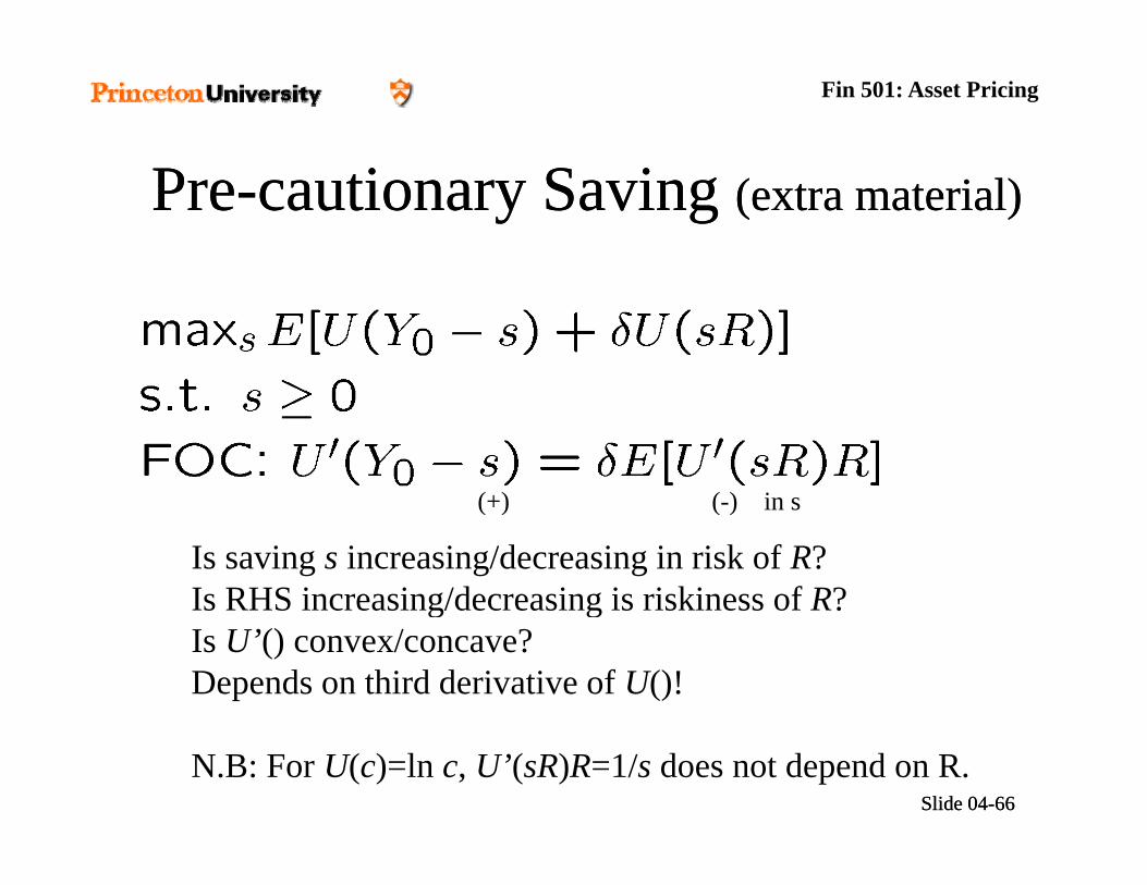
PrePre--cautionary Saving cautionary Saving (extra material)(extra material)
(+) ( ) in s
Is saving s increasing/decreasing in risk of R?Is RHS increasing/decreasing is riskiness of R?
(+) (-) in s
Is RHS increasing/decreasing is riskiness of R?Is U’() convex/concave?Depends on third derivative of U()!
Slide 04Slide 04--6666N.B: For U(c)=ln c, U’(sR)R=1/s does not depend on R.

Fin 501: Asset Pricing
PP ti S iti S i2 effects: Tomorrow consumption is more volatile
PrePre--cautionary Saving cautionary Saving (extra material)(extra material)
2 effects: Tomorrow consumption is more volatile• consume more today, since it’s not risky• save more for precautionary reasons
AR~ BR~
~~
Theorem 4.7 (Rothschild and Stiglitz,1971) : Let , be two return distributions with identical means such that
eRR AB +=
R~ R~
, (where e is white noise) and let sA and sB be, respectively, the savings out of Y0 corresponding to the return distributions andAR BR
0)Y('R R ≤0)Y('R R ≥
return distributions and .If and RR(Y) > 1, then sA < sB ;If and RR(Y) < 1, then sA > sB
Slide 04Slide 04--6767
Fin 501: Asset Pricing
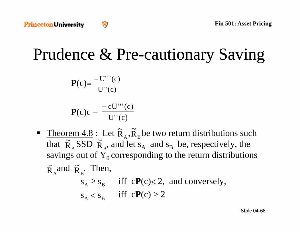
Prudence & PrePrudence & Pre--cautionary Savingcautionary Saving
)c(''U)c('''U−
=P(c)
Th 4 8 L t b t t di t ib ti h
)c(''U
)c('''cU−P(c)c =
~ ~Theorem 4.8 : Let , be two return distributions such that SSD , and let sA and sB be, respectively, the savings out of Y0 corresponding to the return distributions
ARAR~ BR~
BR
0
and . Then,iff cP(c) 2, and conversely,
BR~AR~
ss BA ≥ ≤
Slide 04Slide 04--6868
iff cP(c) > 2 ss BA <

Fin 501: Asset Pricing
O iO i Ri k P fRi k P fOverview: Overview: Risk PreferencesRisk Preferences
1.1. StateState--byby--state dominancestate dominance2.2. Stochastic dominanceStochastic dominance [DD4][DD4]
3.3. vNMvNM expected utility theoryexpected utility theorya)a) IntuitionIntuition [L4][L4]
b)b) A i ti f d tiA i ti f d tib)b) Axiomatic foundationsAxiomatic foundations [DD3][DD3]
4.4. Risk aversion coefficients and Risk aversion coefficients and pportfolio choice ortfolio choice [DD4,5,L4][DD4,5,L4]
55 Prudence coefficient and precautionary savingsPrudence coefficient and precautionary savings [DD5][DD5]5.5. Prudence coefficient and precautionary savings Prudence coefficient and precautionary savings [DD5][DD5]
6.6. MeanMean--variance preferencesvariance preferences [L4.6][L4.6]
Slide 04Slide 04--6969

Fin 501: Asset Pricing
MM i P fi P fMeanMean--variance Preferencesvariance Preferences
Early researchers in finance, such as Markowitz and Sharpe, used just the mean and the variance of the return rate of an asset to describe it.Mean-variance characterization is often easier than using an vNM utility functionBut is it compatible with vNM theory?The answer is yes … approximately … under some conditions.
Slide 04Slide 04--7070
Fin 501: Asset Pricing
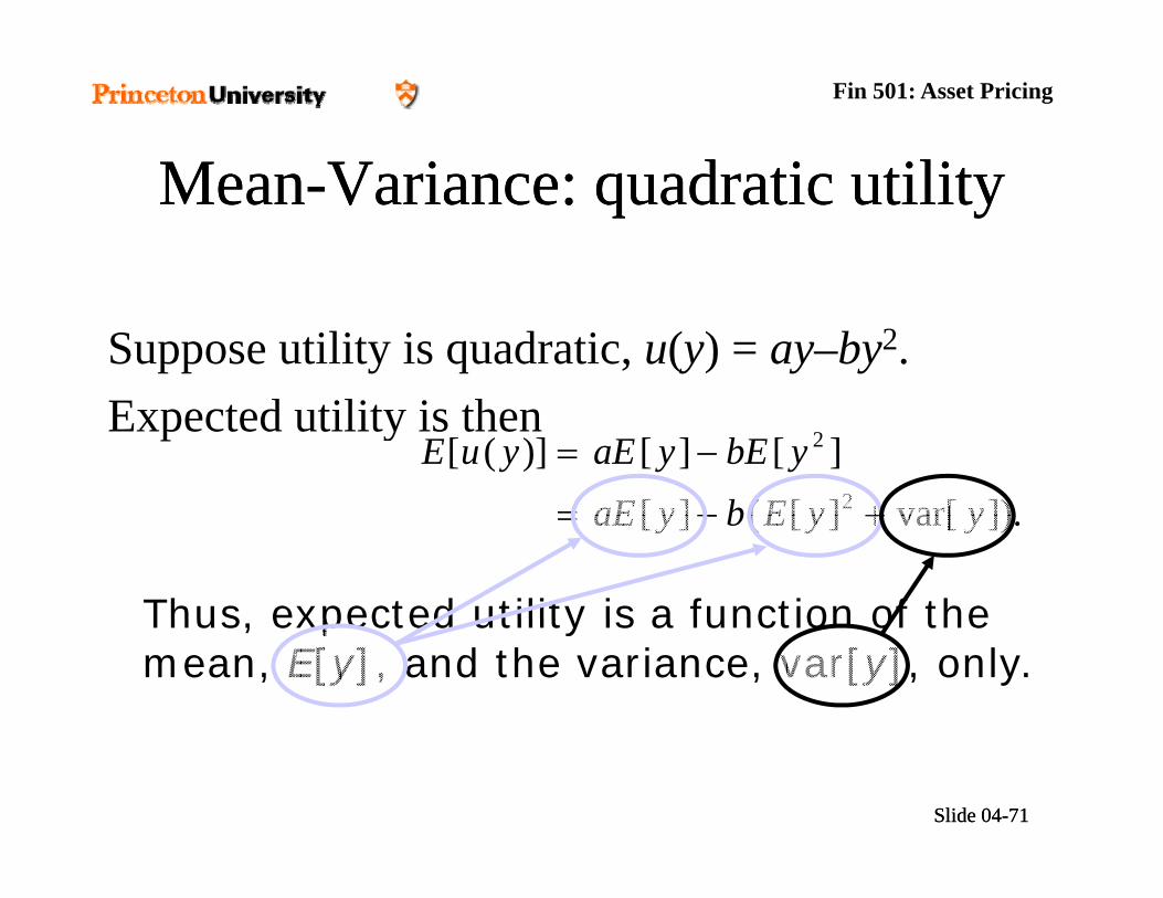
MM V i d ti tilitV i d ti tilitMeanMean--Variance: quadratic utilityVariance: quadratic utility
Suppose utility is quadratic, u(y) = ay–by2.Expected utility is then
])[][(][][][)]([
2
2
EbEybEyaEyuE −=
]).var[][(][ 2 yyEbyaE +−=
Thus expected utility is a function of the Thus, expected utility is a function of the mean, E[y], and the variance, var[y], only.
Slide 04Slide 04--7171
Fin 501: Asset Pricing
MM V i j i t lV i j i t lMeanMean--Variance: joint normalsVariance: joint normals
Suppose all lotteries in the domain have normally distributed prized. (independence is not needed).
Thi i i fi iThis requires an infinite state space.Any linear combination of normals is also normal.The normal distribution is completely described by itsThe normal distribution is completely described by its first two moments.Hence, expected utility can be expressed as a function ofHence, expected utility can be expressed as a function of just these two numbers as well.
Slide 04Slide 04--7272

Fin 501: Asset Pricing
MeanMean--Variance: Variance: ee V ce:V ce:linear distribution classeslinear distribution classes
Generalization of joint nomarls.Consider a class of distributions F1, …, Fn with the f ll ifollowing property:
for all i there exists (m,s) such that Fi(x) = F1(a+bx) for all x.
Thi i ll d li di t ib ti lThis is called a linear distribution class.It means that any Fi can be transformed into an Fj by an appropriate shift (a) and stretch (b)appropriate shift (a) and stretch (b).Let yi be a random variable drawn from Fi. Let μi = E{yi} and σ 2 = E{(y μ )2} denote the mean and the var of y
Slide 04Slide 04--7373
and σi2 = E{(yi–μi)2} denote the mean and the var of yi.

Fin 501: Asset Pricing
MeanMean--Variance: Variance: ee V ce:V ce:linear distribution classeslinear distribution classes
Define then the random variable x = (yi–μi)/σi. We denote the distribution of x with F.Note that the mean of x is 0 and the variance is 1, and F is part of the same linear distribution class.pMoreover, the distribution of x is independent of which i we start with.
)()(∫+∞
zdFzv i
We want to evaluate the expected utility of yi ,
Slide 04Slide 04--7474
.)()(∫ ∞−zdFzv i

Fin 501: Asset Pricing
MeanMean--Variance: Variance: ee V ce:V ce:linear distribution classeslinear distribution classes
∫∫+∞+∞
But yi = μi + σi x, thus
).,(:
)()()()(
ii
iii
u
zdFzvzdFzv
σμ=
σ+μ= ∫∫+∞
∞−
+∞
∞−
).,(: iiu σμ
The expected utility of all random variables d f h l d bdrawn from the same linear distribution class can be expressed as functions of the mean and the standard deviation only
Slide 04Slide 04--7575
mean and the standard deviation only.

Fin 501: Asset Pricing
MM V i ll i kV i ll i kMeanMean--Variance: small risksVariance: small risks
Justification for mean-variance for the case of small risks.use a second order (local) Taylor approximation of vNMuse a second order (local) Taylor approximation of vNM U(c).If U(c) is concave, second order Taylor approximation is a ( ) , y ppquadratic function with a negative coefficient on the quadratic term.E i f d i ili f i bExpectation of a quadratic utility function can be evaluated with the mean and variance.
Slide 04Slide 04--7676

Fin 501: Asset Pricing
MeanMean Variance: small risksVariance: small risksMeanMean--Variance: small risksVariance: small risks
Let f : R R be a smooth function The TaylorLet f : R R be a smooth function. The Taylor approximation is
+−
+−
+≈!2
)()(''
!1)(
)(')()(2
00
10
00xx
xfxx
xfxfxf
L+−
!3)(
)('''3
00
xxxf
Use Taylor approximation for E[u(x)].
Slide 04Slide 04--7777

Fin 501: Asset Pricing
MeanMean Variance: small risksVariance: small risksMeanMean--Variance: small risksVariance: small risksSince E[u(w+x)] = u(cCE), this simplifies to
.2
)var()( xwRcw ACE ≈−
w – cCE is the risk premium.
W h th t th i k i i We see here that the risk premium is approximately a linear function of the variance of the additive risk with the variance of the additive risk, with the slope of the effect equal to half the coefficient of absolute risk.
Slide 04Slide 04--7878

Fin 501: Asset Pricing
MeanMean Variance: small risksVariance: small risksMeanMean--Variance: small risksVariance: small risksThe same exercise can be done with a multiplicative risk.Let y = gw, where g is a positive random variable with unit mean.D i th t b f l d tDoing the same steps as before leads to
,)var()(1 gwRR≈−κ
where κ is the certainty equivalent growth rate, u( w) E[u(gw)]
,2
)(
u(κw) = E[u(gw)].
The coefficient of relative risk aversion is relevant for multiplicative risk absolute risk
Slide 04Slide 04--797912:30 Lecture Risk Aversion
relevant for multiplicative risk, absolute risk aversion for additive risk.

Fin 501: Asset Pricing
E t t i l f ll !E t t i l f ll !Extra material follows!Extra material follows!
Slide 04Slide 04--8080

Fin 501: Asset Pricing
Joint savingJoint saving--portfolio problemportfolio problem• Consumption at t=0 and t=1. (savings decision)• Asset structure
– One risk free bond with net return rf
– One risky asset (a = quantity of risky assets)
))rr~(a)r1(s(EU)sY(Umax ff0}sa{−++δ+− (4.7)
y ( q y y )
}s,a{( )
FOC:s: U’(ct) = δ E[U’(ct+1)(1+rf)]a: E[U’(c )(r r )] = 0
Slide 04Slide 04--8181
a: E[U (ct+1)(r-rf)] = 0

Fin 501: Asset Pricing
for CRRA utility functions
( ) 0)r1()]rr~(a)r1(s[E)1()sY( fff0 =+−++δ+−− γ−γ−s:
[ ] 0)rr~())rr~(a)r1(s(E fff =−−++ γ−a:
Where s is total saving and a is amount invested in risky assetWhere s is total saving and a is amount invested in risky asset.
Slide 04Slide 04--8282

Fin 501: Asset Pricing
M ltiM lti i d S ttii d S ttiMultiMulti--period Settingperiod Setting
Canonical framework (exponential discounting)U(c) = E[ ∑ βt u(ct)]
prefers earlier uncertainty resolution if it affect actionindifferent, if it does not affect action
Time-inconsistent (hyperbolic discounting)Special case: β−δ formulation
U(c) = E[u(c ) + β ∑ δt u(c )]U(c) = E[u(c0) + β ∑ δt u(ct)]Preference for the timing of uncertainty resolution
recursive utility formulation (Kreps Porteus 1978)
Slide 04Slide 04--8383
recursive utility formulation (Kreps-Porteus 1978)

Fin 501: Asset Pricing
M ltiM lti i d P tf li Ch ii d P tf li Ch iMultiMulti--period Portfolio Choiceperiod Portfolio Choice
Theorem 4.10 (Merton, 1971): Consider the above canonical ( )multi-period consumption-saving-portfolio allocation problem. Suppose U() displays CRRA, rf is constant and {r} is i.i.d. Then a/s is time invariant
Slide 04Slide 04--8484
Then a/st is time invariant.

Fin 501: Asset Pricing
Digression:Digression: Preference for the Preference for the g ess o :g ess o : e e e ce o ee e e ce o etiming of uncertainty resolutiontiming of uncertainty resolution
$100π $150
$100
$100π
$ 25$150
0
$100$ 25Kreps-Porteus
Early (late) resolution if W(P1,…) is convex (concave)
Slide 04Slide 04--8585
Marginal rate of temporal substitution risk aversion