Abstract – This paper serves to describe the

development and application of a web based, low cost, user friendly Inventory Analysis Tool for stock availability optimization and enhanced delivery performance. The inventory optimization attempts to find dynamically the best inventory policy and safety stock for Stock Keeping Units with independent demands. The analysis is based on supply and demand data, which includes forecast variability and measurements. Important supply chain parameters are modeled and estimated with graphical visualization to identify potential opportunities for improvement. The tool gathers all historical and up-to-date information to effectively track the replenishment level, safety stock level and re-order level of finished goods within minutes. A case study from National Heart Center Singapore on the use of the tool is presented. The results should encourage more inventory managers to use the tool to lower inventory dollar level and put forecasting error in check and control.

Keywords – Forecast, inventory analysis tool, inventory

policy, safety stock, supply chain parameters

I. INTRODUCTION Many companies are using demand planning applications and systems such as Enterprise Resource Planning (ERP) or advanced planning and scheduling system (APS) in their operations. Very often, static inventory target parameters are applied broadly across different products or Stock Keeping Units (SKU) regardless of whether actual supply chain demand and supply parameters have changed or not. The key reason for adopting static inventory target is that inventory managers are getting more responsibilities in their work scope and comprehensive inventory analysis by SKU is difficult to accomplish within a planning cycle. Demand characteristics can change within planning cycle, and failure to monitor and adjust inventory policy can cost substantial capital to be tied up in inventory. A systematic way of analysis and optimizing inventory will help to reduce costs and improve customer satisfaction. This paper will discuss the development of an inventory analysis tool to help company to do inventory analysis timely and dynamically seeking inventory reduction opportunities. A case study with National Heart Center is described and serves as a reference for future application. The objective of the tool is to enable inventory analysis and targets set within a short time of within minutes instead of days or weeks. The correct setting of inventory

targets in ERP application or simply control the inventory targets manually will mean great cost saving opportunity. The inventory analysis tool significantly improves the ability to effectively monitor inventory by making inventory analysis processes much more guided, automated and comprehensive through the use of user friendly step by step guidance, coupled with graphical visualizations and numerical interpretations. The National Heart Centre (NHC) material management team supports is responsible for purchasing and carrying inventory for cardiac wards, laboratory and operating theatres. The SKU it carries includes medical administrative consumables and supplies. Examples of inventory it carries include ward procedure charge form, electrode, pillowcases and masks. The inventory analysis tool enables NHC to analyze the inventory targets and forecast accuracy for those SKU with independent demand across different inventory polices so that the most suitable inventory policy can be selected. Each independent demand SKU can be viewed singly and forecast pattern can be studied [1]. Independent demand systems are used to determine levels of finished goods inventory and used by retail, wholesale, bank, hospital, service and distribution industry [2].

II. APPROACH The inventory analysis tool takes into account inventory review period, delivery frequency of the supplier, lead time, demand variability or forecast error and any fixed order quantity. Base on user data, the historical inventory, forecast and demand are analyzed to decide the SKU to prioritize analysis. Subsequently, a normality test will be done to ascertain if the inventory movement can be described by a normal distribution. Thereafter, inventory analysis is then done on the inventory movement to obtain average stock level, inventory reduction and cost savings based on different well known inventory policies. Fig.1 shows the screen capture of the inventory analysis tool portal showing the typical work flow or steps.

Implementation of Inventory Analysis Tool for Optimization and Policy Selection

Siong Sheng Chin, Edmund Chan, Terence Yeo School of Engineering, Republic Polytechnic, Singapore School of Engineering, Republic Polytechnic, Singapore Material Management, National Heart Centre, Singapore

(chin_siong_sheng@rp.sg)

978-1-4244-2330-9/08/$25.00 ©2008 IEEE 1407

Fig. 1 Screen capture of the inventory analysis tool portal showing the recommended steps A. Step 1: Upload Data

The user is requested to upload demand, inventory, supply chain parameters and forecast if any, using a standard Microsoft Excel (MS Excel) template. Fig.2 shows the screen capture of the data uploading for all SKU that user is interested to analyze.

Fig. 2 Screen capture of the data uploading B. Step 2: ABC Analysis The tool allows ABC analysis [2] to be performed on different SKU so that the more important SKU can be selected for further inventory reduction through different inventory policies in step 3 and step 4. ABC analysis consists of classifying SKU in “A”, “B” and “C” categories. “A” items are typically 20% of the items accounting for 80% of the inventory value [3]. “B” items are typically an additional 30% of the items accounting for 15% of the inventory value [3]. “C” items are typically 50% of the items accounting for 5% of the inventory value [3]. C. Step 3: Normal Distribution Analysis Inventory policy calculations are based on normality distribution assumptions in inventory movement. The normality assumption of inventory movement may not be true. As such, it is important to check, and try and describe the inventory movement by normality distribution before further analysis on inventory policies can be done. There are two main approaches to checking normal distribution assumptions. One involves empirical procedure which is based on intuitive and graphical

properties [4]. The other involves use of Goodness of Fit (GoF) test which is more formal and consists of statistically procedures [4]. Among the GoF procedures for small samples, the Anderson-Darling (AD) test is used in checking the normality distribution assumption for the demand data and forecast error data. AD GoF test for Normality can be done using software packages Minitab or MS Excel [4]. If the AD test statistic is greater than critical value (CV), the distribution of the demand or forecast error data does not follow normal distribution [4]. When the demand or forecast error data distribution is not normal, the demand for consecutive period is aggregated. If a weekly demand cannot be described using a normal distribution, a consolidated bi-weekly demand is used for normality analysis. If the bi-weekly demand cannot be described by the normal distribution, a 3-week consolidated demand data is used. The iteration will continue till a demand or forecast error data set is normally distributed.

Fig. 3 Screen capture of the normality test Fig. 3 shows the output of the normality test when AD test statistic is less than CV. The inventory analysis tool is capable of testing and evaluating the normality assumptions on the demand data or forecast error data. It suggests the number of periods of demand to be consolidated to smoothen the demand and hence making the normality assumption valid in estimating the safety stock. D. Step 4: Inventory Analysis In a typical inventory analysis model, as shown in Fig. 4, the reorder level is triggered by the information from the system that the stock is low taking into the supply lead time [5]. Safety stock or minimum stock level is vital for ensuring that there is warning of low stocks [5].

Quan

tity in

Stoc

k

Time

Safety Stock

Reorder Level

Target Stock level

OrderDelivery

Fig. 4 Basic model for inventory analysis

Proceedings of the 2008 IEEE ICMIT

1408

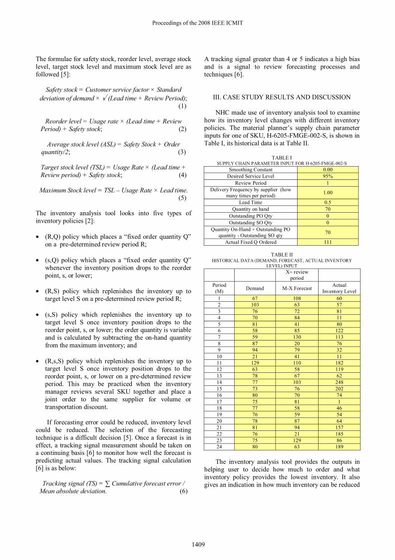
The formulae for safety stock, reorder level, average stock level, target stock level and maximum stock level are as followed [5]:

Safety stock = Customer service factor × Standard deviation of demand × √ (Lead time + Review Period); (1)

Reorder level = Usage rate × (Lead time + Review

Period) + Safety stock; (2)

Average stock level (ASL) = Safety Stock + Order quantity/2; (3)

Target stock level (TSL) = Usage Rate × (Lead time + Review period) + Safety stock; (4)

Maximum Stock level = TSL – Usage Rate × Lead time. (5)

The inventory analysis tool looks into five types of inventory policies [2]: • (R,Q) policy which places a “fixed order quantity Q”

on a pre-determined review period R;

• (s,Q) policy which places a “fixed order quantity Q” whenever the inventory position drops to the reorder point, s, or lower;

• (R,S) policy which replenishes the inventory up to

target level S on a pre-determined review period R;

• (s,S) policy which replenishes the inventory up to target level S once inventory position drops to the reorder point, s, or lower; the order quantity is variable and is calculated by subtracting the on-hand quantity from the maximum inventory; and

• (R,s,S) policy which replenishes the inventory up to

target level S once inventory position drops to the reorder point, s, or lower on a pre-determined review period. This may be practiced when the inventory manager reviews several SKU together and place a joint order to the same supplier for volume or transportation discount.

If forecasting error could be reduced, inventory level could be reduced. The selection of the forecasting technique is a difficult decision [5]. Once a forecast is in effect, a tracking signal measurement should be taken on a continuing basis [6] to monitor how well the forecast is predicting actual values. The tracking signal calculation [6] is as below:

Tracking signal (TS) = ∑ Cumulative forecast error / Mean absolute deviation. (6)

A tracking signal greater than 4 or 5 indicates a high bias and is a signal to review forecasting processes and techniques [6].

III. CASE STUDY RESULTS AND DISCUSSION

NHC made use of inventory analysis tool to examine

how its inventory level changes with different inventory policies. The material planner’s supply chain parameter inputs for one of SKU, H-6205-FMGE-002-S, is shown in Table I, its historical data is at Table II.

TABLE I

SUPPLY CHAIN PARAMETER INPUT FOR H-6205-FMGE-002-S Smoothing Constant 0.00

Desired Service Level 95% Review Period 1

Delivery Frequency by supplier (how many times per period) 1.00

Lead Time 0.5 Quantity on hand 70

Outstanding PO Qty 0 Outstanding SO Qty 0

Quantity On-Hand + Outstanding PO quantity - Outstanding SO qty 70

Actual Fixed Q Ordered 111

TABLE II HISTORICAL DATA (DEMAND, FORECAST, ACTUAL INVENTORY

LEVEL) INPUT X= review

period

Period (M) Demand M-X Forecast Actual

Inventory Level 1 67 108 60 2 103 63 57 3 76 72 81 4 70 84 11 5 81 41 80 6 58 85 122 7 59 130 113 8 87 20 76 9 94 79 32 10 21 41 11 11 129 110 182 12 63 58 119 13 78 67 62 14 77 103 248 15 73 76 202 16 80 70 74 17 75 81 1 18 77 58 46 19 76 59 54 20 78 87 64 21 81 94 157 22 76 21 185 23 75 129 86 24 80 63 189

The inventory analysis tool provides the outputs in

helping user to decide how much to order and what inventory policy provides the lowest inventory. It also gives an indication in how much inventory can be reduced

Proceedings of the 2008 IEEE ICMIT

1409

based on current policy. Table III shows the data output from the inventory analysis tool.

TABLE III DATA OUTPUT FOR H-6205-FMGE-002-S UNDER NHC’S CURRENT

POLICY (R, Q)

Suggested Order Quantity 203

Average Demand 76

Average Actual Inventory 114

The tracking signal for the forecast of H-6205-FMGE-002-S is shown as red line in Fig. 6. As the tracking signal is fluctuating within -4 to +4, the forecast is reasonably well in predicting the demand. No specific forecast bias identified.

-3

-2

-1

0

1

2

3

4

0

20

40

60

80

100

120

140

1 2 3 4 5 6 7 8 9 10 11 12 13 14 15 16 17 18 19 20 21 22 23 24

Tracking signal

Demand

Period

H-6205-FMGE-002-S

Demand

M-X Forecast

TS

Fig. 6 Tracking signal of forecast for H-6205-FMGE-002-S Fig. 7, Fig. 8, Fig.9, Fig.10 and Fig.11 show the graphical outputs of the actual demand, forecast, actual inventory level and average stock level (ASL), under different inventory policies. For inventory policies (R, S), (s, S) and (R, s, S), target stock level (TSL) is included. For inventory policies (R, S), (R, Q) and (R, s, S), safety stock level is included. For inventory policy (s, S), (s, Q), and (R, s, S) reorder level is included.

Fig. 7 Graphical output of H-6205-FMGE-002-S under (R, Q) inventory policy Fig. 7 shows that inventory level of H-6205-FMGE-002-S is fluctuating around average stock level (ASL). The fluctuation is large relative to safety stock for period 13 to period 17, but improving from period 18 to 24.

Fig. 8 Graphical output of H-6205-FMGE-002-S under (s, Q) inventory policy Fig. 8 shows that the forecast is fluctuating more from period 21 to period 24, while the demand remained relatively stable from period 13 to period 24. From period 21 onwards, the material planner seems to have estimated the reorder point correctly. The planner may look into improving the cycle stock by reducing the order quantity Q and understand the root cause of increasing forecasting error.

Fig. 9 Graphical output of H-6205-FMGE-002-S under (R, S) inventory policy Fig. 9 shows that the planner has exceeded the target stock level (TSL) and above the safety stock target from period 13 to period 20 significantly. With the knowledge of the TSL and safety stock, the planner will plan the inventory more confidently in the future.

0

50

100

150

200

250

1 3 5 7 9 11 13

Qua

ntity

Period

s,S Actual

Demand

Forecast

Actual

Inventory

Level

ReOrder

Point

ASL

TSL

Fig. 10 Graphical output of H-6205-FMGE-002-S under (s, S) inventory policy

Quantity

0

50

100

150

200

250

13 15 17 19 21 23 253

Period

R,S ActualDemand

Forecast

Actual

Inventory Level

SafetyStock

ASL

TSL

0

50

100

150

200

250

13 15 17 19 21 23 25

Quantity

Period

s,Q Actual

Demand

Forecast

Actual Inventory Level

ReorderPoint

ASL

0

50

100

150

200

250

13 15 17 19 21 23 25

Quantity

Period

R,Q ActualDemand

Forecast

Actual

Inventory Level

SafetyStock

ASL

Proceedings of the 2008 IEEE ICMIT

1410

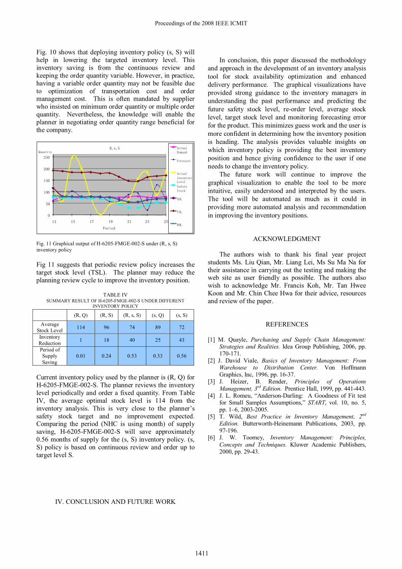
Fig. 10 shows that deploying inventory policy (s, S) will help in lowering the targeted inventory level. This inventory saving is from the continuous review and keeping the order quantity variable. However, in practice, having a variable order quantity may not be feasible due to optimization of transportation cost and order management cost. This is often mandated by supplier who insisted on minimum order quantity or multiple order quantity. Nevertheless, the knowledge will enable the planner in negotiating order quantity range beneficial for the company.

Fig. 11 Graphical output of H-6205-FMGE-002-S under (R, s, S) inventory policy Fig 11 suggests that periodic review policy increases the target stock level (TSL). The planner may reduce the planning review cycle to improve the inventory position.

TABLE IV SUMMARY RESULT OF H-6205-FMGE-002-S UNDER DIFFERENT

INVENTORY POLICY

Current inventory policy used by the planner is (R, Q) for H-6205-FMGE-002-S. The planner reviews the inventory level periodically and order a fixed quantity. From Table IV, the average optimal stock level is 114 from the inventory analysis. This is very close to the planner’s safety stock target and no improvement expected. Comparing the period (NHC is using month) of supply saving, H-6205-FMGE-002-S will save approximately 0.56 months of supply for the (s, S) inventory policy. (s, S) policy is based on continuous review and order up to target level S.

IV. CONCLUSION AND FUTURE WORK

In conclusion, this paper discussed the methodology and approach in the development of an inventory analysis tool for stock availability optimization and enhanced delivery performance. The graphical visualizations have provided strong guidance to the inventory managers in understanding the past performance and predicting the future safety stock level, re-order level, average stock level, target stock level and monitoring forecasting error for the product. This minimizes guess work and the user is more confident in determining how the inventory position is heading. The analysis provides valuable insights on which inventory policy is providing the best inventory position and hence giving confidence to the user if one needs to change the inventory policy. The future work will continue to improve the graphical visualization to enable the tool to be more intuitive, easily understood and interpreted by the users. The tool will be automated as much as it could in providing more automated analysis and recommendation in improving the inventory positions.

ACKNOWLEDGMENT The authors wish to thank his final year project students Ms. Liu Qian, Mr. Liang Lei, Ms Su Ma Na for their assistance in carrying out the testing and making the web site as user friendly as possible. The authors also wish to acknowledge Mr. Francis Koh, Mr. Tan Hwee Koon and Mr. Chin Chee Hwa for their advice, resources and review of the paper.

REFERENCES

[1] M. Quayle, Purchasing and Supply Chain Management: Strategies and Realities. Idea Group Publishing, 2006, pp. 170-171.

[2] J. David Viale, Basics of Inventory Management: From Warehouse to Distribution Center. Von Hoffmann Graphics, Inc, 1996, pp. 16-37.

[3] J. Heizer, B. Render, Principles of Operations Management, 3rd Edition. Prentice Hall, 1999, pp. 441-443.

[4] J. L. Romeu, “Anderson-Darling: A Goodness of Fit test for Small Samples Assumptions,” START, vol. 10, no. 5, pp. 1–6, 2003-2005.

[5] T. Wild, Best Practice in Inventory Management, 2nd Edition. Butterworth-Heinemann Publications, 2003, pp. 97-196.

[6] J. W. Toomey, Inventory Management: Principles, Concepts and Techniques. Kluwer Academic Publishers, 2000, pp. 29-43.

(R, Q) (R, S) (R, s, S) (s, Q) (s, S)

Average Stock Level 114 96 74 89 72

Inventory Reduction 1 18 40 25 43

Period of Supply Saving

0.01 0.24 0.53 0.33 0.56

0

50

100

150

200

250

13 15 17 19 21 23 25

Quantity

Period

R,s,S ActualDemand

Forecast

ActualInventory Level

SafetyStock

ASL

TSL

ROL

Proceedings of the 2008 IEEE ICMIT

1411