04.2013 jis tobam properties of the most diversified portfolio · choueifaty and coignard (journal...
TRANSCRIPT
Journal of Investment Strategies Volume 2/Number 2, Spring 2013 (1–22)
Properties of the most diversified portfolio
Yves Choueifaty
TOBAM, 20 rue Quentin Bauchart, 75008 Paris, France;
email: [email protected]
Tristan Froidure
TOBAM, 20 rue Quentin Bauchart, 75008 Paris, France;
email: [email protected]
Julien Reynier
TOBAM, 20 rue Quentin Bauchart, 75008 Paris, France;
email: [email protected]
(Received November 20, 2012; accepted January 31, 2013)
This paper expands upon “Toward Maximum Diversification”, a 2008 paper by
Choueifaty and Coignard (Journal of Portfolio Management 35(1), 40–51). We
present new mathematical properties of the diversification ratio and most diver-
sified portfolio (MDP), and investigate the optimality of the MDP in a mean-
variance framework. We also introduce a set of “portfolio invariance proper-
ties”, providing the basic rules an unbiased portfolio construction process should
respect. In the light of these rules, the MDP is then compared with popular method-
ologies (equal weights, equal risk contribution, minimum variance), and their
performance is investigated over the past decade, using the MSCI World as the
reference universe. We believe that the results obtained in this paper show that
the MDP is a strong candidate for being the undiversifiable portfolio, and as such
delivers investors the full benefit of the equity premium.
1 INTRODUCTION
Ever since its introduction in the 1960s, the capital asset pricing model (CAPM) has
come under intense scrutiny. In particular, the efficiency of the market capitalization
weighted index has been questioned,with academics andpractitioners offering numer-
ous investment alternatives. In a seminal paper, Haugen and Baker (1991) concisely
proclaimed that “matching the market is an inefficient investment strategy”. They
The authors would like to thank Robert Arnott, Jason Hsu and particularly the late Robert Haugen
for their very helpful feedback, remarks and encouragements. We would also like to thank our
colleagues at TOBAM for their instrumental contributions and great support.
1

2 Y. Choueifaty et al
argued that theory can still predict cap-weighted portfolios to be inefficient invest-
ments, even assuming that investors rationally optimize the relationship between risk
and expected return in equilibrium, in an “informationally efficient” capital market.
Putting theory into practice, Haugen and Baker presented one of the first empirical
studies of the minimum-variance portfolio. Over the period 1972–89, this portfolio
delivered returns equal to or greater than those of a broad market cap-weighted index
of US stocks, while achieving consistently lower volatility, thus demonstrating the
ex post inefficiency of the market cap-weighted index. Nearly fifteen years later,
Arnott et al (2005) created indexes with alternative measures of company size based
on fundamental metrics. They showed that such indexes were “more mean-variance
efficient” than market cap-weighted indexes, further challenging the CAPM. Subse-
quently, Choueifaty (2006) introduced the concept of maximum diversification, via a
formal definition of portfolio diversification: the diversification ratio (DR).Choueifaty
further went on to describe the portfolio which maximizes the DR – the most diver-
sified portfolio (MDP) – as an efficient alternative to the market cap-weighted index.
This paper expands upon Choueifaty and Coignard (2008), which introduced the
concepts of DR and MDP to a broad audience. First, we explore the mathematical
properties of the DR. We also establish a new equivalent definition of the long-only
MDP, and generalize the condition for the optimality of the MDP in a mean-variance
framework. Next, we compare theMDPwith threewell-known long-only quantitative
portfolio construction approaches: the equal-weighted (EW), equal-risk-contribution
(ERC) (Maillard et al 2010) and minimum-variance (MV) portfolios (Haugen and
Baker 1991; Clarke et al 2006).We introduce a set of basic invariance properties that
an unbiased portfolio construction process should respect, and then examine each
approach in light of these properties, using synthetic examples. Finally, using one of
the broadest equity universes available – the MSCI World – we study the empirical
performance of the four portfolios over the past decade.
2 PROPERTIES OF THE DIVERSIFICATION RATIO
2.1 Definition
Numerous definitions of diversifications have been proposed since the seminal work
of Markowitz (1952). Choueifaty (2006) proposed an actual measure of portfolio
diversification, called the DR, which he defined as the ratio of the portfolio’s weighted
average volatility to its overall volatility. This measure embodies the very nature of
diversification, whereby the volatility of a long-only portfolio of assets is less than or
equal to the weighted sum of the assets’ volatilities. As such, the DR of a long-only
portfolio is greater than or equal to 1, and equals unity for a single-asset portfolio.
Consider, for example, an equal-weighted portfolio of two independent assets with
Journal of Investment Strategies Volume 2/Number 2, Spring 2013

Properties of the most diversified portfolio 3
the same volatility: its DR is equal top
2, and top
N for N independent assets.1 In
essence, the DR of a portfolio measures the diversification gained from holding assets
that are not perfectly correlated. We formalize this intuition by introducing a formal
definition as well as establishing several properties of the DR. Note that all portfolios
in this paper are constrained to be long-only, unless otherwise stated.2
We consider a universe of N risky single assets fS1; : : : ; SN g, with volatility � D.�i /, correlation matrix C D .�i;j / and covariance matrix ˙ D .�i;j �i�j /, with
1 6 i; j 6 N . Let w D .wi / be the weights of a long-only portfolio, � .w/ its
volatility, and hw j � i DP
i wi�i its average volatility. The diversification ratio
DR.w/ of a portfolio is defined as the ratio of its weighted average volatility and its
volatility,
DR.w/ D hw j � i�.w/
: (2.1)
2.2 DR decomposition
It is intuitive that portfolios with “concentrated” weights and/or highly correlated
holdings would be poorly diversified, and hence be characterized by relatively low
DRs. Here we formalize this intuition by decomposing the DR of a portfolio into its
weighted-correlation andweighted-concentrationmeasures.As shown inAppendixA,
the DR decomposition is
DR.w/ D Œ�.w/.1 CR.w//C CR.w/� 1=2; (2.2)
where �.w/ is the volatility-weighted average correlation of the assets in the portfolio,
�.w/ DP
i¤j .wi�iwj �j /�i;jP
i¤j .wi�iwj �j /; (2.3)
and CR.w/ is the volatility-weighted concentration ratio (CR) of the portfolio, with
CR.w/ DP
i .wi�i /2
.P
i wi�i /2
: (2.4)
A fully concentrated long-only portfolio has unit CR (a one asset portfolio), while
an equal volatility weighted portfolio has the lowest CR, equal to the inverse of the
1 In effect, the average volatility of the assets is equal to their common volatility, and the volatility of
the portfolio equals their common volatility divided by the square root of the number of assets. We
refer the reader to the “Definition of the diversification ratio” section of Choueifaty and Coignard
(2008), for more examples.2 Definitions are provided accordingly.
Research Paper www.risk.net/journal
4 Y. Choueifaty et al
number of assets it contains.3 The CR introduces a generalization of the Herfindahl–
Hischman index (Rhoades 1993; Bouchaud and Potters 2009, p. 205) used, for exam-
ple, by US authorities as a sector concentration measure. In effect, the CR measures
not only the concentration of weights, but also the concentration of risks; assets are
weighted proportionally to their volatilities.
The above DR decomposition explicitly shows that the DR increases when the
average correlation and/or the CR decreases. In the extreme, if correlations increase
to unity, the DR is equal to 1, regardless of the value of the CR, as portfolios of
assets are no more diversified than a single asset. We note that when pairwise asset
correlations are equal, the DR varies only via the CR, and maximizing the DR is
equivalent to minimizing the CR.
2.3 The DR as a measure of degrees of freedom
We provide an intuitive interpretation of the DR, by first considering a universe of F
independent risk factors, and a portfoliowhose exposure to each risk factor is inversely
proportional to the factor’s volatility. Such a portfolio allocates its risk budget equally
across all risk factors, andwill have aDR squared (DR2) equal toF .4As such, its DR2
is equal to the number of independent risk factors, or degrees of freedom, represented
in the portfolio. Therefore, the DR2 of any portfolio of assets can be interpreted as
the number F of independent risk factors, necessary for a portfolio that allocates
equal risk to independent risk factors, to achieve the same DR. As such, F can be
interpreted as the effective number of independent risk factors, or degrees of freedom,
represented in the portfolio.
For example, the DR of an index, such as the MSCI World, was 1.7 as of the end
of 2010, implying that a passive MSCI World investor would have been effectively
exposed to 1:72 � 3 independent risk factors, in our interpretation. Taking this a step
further, if we seek to maximize the DR, the resulting DR would equal the square root
of the effective number of independent risk factors available in the entire market. At
the end of 2010, this resulted in a DR of 2.6, or 2:62 � 7 effective degrees of freedom.
An interpretation of this result is that the market cap-weighted index misses out on
the opportunity to effectively diversify across about four additional independent risk
factors.
3 The Herfindal index attains its minimum value for an equal-weighted portfolio. In our case, it
suffices to rescale the portfolio weights by their associated volatilities to obtain this result.4 In effect, noting c the proportionality constant between the weights of the portfolio and the inverse
of the volatilities, the numerator of the DR equals c times F , while its denominator equals c times
the square root of F .
Journal of Investment Strategies Volume 2/Number 2, Spring 2013
Properties of the most diversified portfolio 5
3 THE MOST DIVERSIFIED PORTFOLIO
3.1 Definition
The attractive properties of the DR naturally lead to the construction of maximally
diversified long-only portfolios, defined as
wMDP D arg max
w2˘ C
DR.w/; (3.1)
where ˘C is the set of long-only portfolios with weights summing to 1.5 As shown
in Appendix B, the long-only MDP always exists and is unique when the covari-
ance matrix ˙ is definite. Furthermore, the portfolio’s weights satisfy the first-order
condition
˙wMDP D �.wMDP/
DR.wMDP/� C �; (3.2)
where the nonnegative (dual) variables � are such that min.�; wMDP/ D 0.
3.2 The core properties of the MDP
An equivalent definition6 of theMDP, which we call the core property of theMDP (1),
provides a very intuitive understanding of its nature.
(1) Any stock not held by the MDP is more correlated to the MDP than any of the
stocks that belong to it. Furthermore, all stocks belonging to the MDP have the
same correlation to it.
This property illustrates that all assets in the universe considered are effectively repre-
sented in the MDP, even if the portfolio does not physically hold them. For example,
an MDP portfolio constructed using S&P 500 stocks may hold approximately 50
stocks. That does not mean, however, that this portfolio is not diversified, as the 450
stocks it does not hold are more correlated to the MDP compared with the 50 stocks it
actually holds. This is consistent with the notion that the MDP is the undiversifiable
portfolio.
5 Note that this section treats the long-only constrainedMDP.We refer the reader to the “Properties”
section of Choueifaty and Coignard (2008) for results addressing the unconstrained (long–short)
case. Also, the objective is finite providing there does not exist a zero volatility portfolio in ˘C.
In an equity context, that amounts to assume there does not exist a long-only, zero risk portfolio
bearing a positive risk premium. This is of course the case when ˙ is definite.6We show inAppendix B that, when the covariance matrix is definite, the MDP is the only portfolio
respecting this property, which uniquely defines the MDP. When this is not the case, all portfolios
respecting this property have maximal diversification, and are fully correlated.
Research Paper www.risk.net/journal
6 Y. Choueifaty et al
The core property of the MDP (1) is established inAppendix B with the help of the
above first-order condition. It is also equivalent to the following alternative definition,
which is more involved, and forms the basis of its proof. For this reason, we call it
the core property of the MDP (2).
(2) The long-onlyMDP is the long-only portfolio such that the correlation between
any other long-only portfolio and itself is greater than or equal to the ratio of
their DRs.7
Equivalently, for any long-only portfolio with weights w:
�w;wMDP >DR.w/
DR.wMDP/: (3.3)
Accordingly, the more diversified a long-only portfolio is, the greater its correlation
with the MDP. Note that when the covariance matrix ˙ is not definite, all portfolios
satisfying the core property (1) or (2), equivalently maximize the DR. As such, (3.3)
also shows that all solutions are equivalent, as they have a correlation of one between
themselves.
3.3 Optimality properties of the MDP in a mean-variance framework
We show in this section that, provided “risk is rewarded” – a central tenet of finance –
maximizing the DR is equivalent to maximizing investors’ ubiquitous mean-variance
utility. In that case, the MDP is the optimal, equilibrium portfolio.8
Consider a homogeneous investment universe of single assets where we have no
reason to believe, ex ante, that any single asset will reward risk more than another.
In this universe, the ex ante Sharpe ratios of single assets are identical, and thus
each asset’s expected excess return (EER) is proportional to its volatility: risk is
homogeneously rewarded. Assume that a risk-free asset is available, with rate rf .
Denoting by r1; : : : ; rN the single assets’ returns and by k a positive constant, single
assets’ EERs satisfy
E.ri / rf D k�i : (3.4)
As such, for any portfolio of single assets with weights w and return rw,
E.rw/ rf DN
X
iD1
wi .E.ri / rf / D khw j � i:
7A similar property was derived in Choueifaty and Coignard (2008) in a simpler unconstrained
(long/short) setting.8 This ideal setting is of course far from reality. Note, however, that the assumptions entertained
here are not prerequisites for the MDP’s outperformance in other contexts, in particular in the real
world.
Journal of Investment Strategies Volume 2/Number 2, Spring 2013
Properties of the most diversified portfolio 7
Using the definition of the diversification ratio, we finally obtain
E.rw/ rf D k�.w/DR.w/: (3.5)
Equation (3.5) shows that portfolios’ EERs are proportional to their volatilities mul-
tiplied by their DRs.9 Dividing both sides of this equation by �.w/ demonstrates that
in this homogenous universe, maximizing the DR is equivalent to maximizing the
Sharpe ratio.
Going a step further, assume that all CAPM assumptions hold as in Sharpe (1991),
whose Nobel lecture includes a very clear, self-contained, exposé of the CAPM. One
central assumption is that “all investors are in agreement concerning expected returns
and (asset) covariances”.When equilibrium prices are attained, both expected returns
and covariances are determined in such a way that markets clear. Let us explore fur-
ther the case where all investors also agree that single assets’ EERs are proportional
to their volatilities. In this setting, assets’EERs depend on volatilities and on the pro-
portionality constant k (constant across assets).10 As such, assuming that equilibrium
prices are attained, both asset covariances and the constant k are determined in equi-
librium. Provided that markets have cleared, we still obtain the security market line
relationship.11 Also, as a risk-free asset is available, the portfolio of risky assets held
by all investors maximizes the Sharpe ratio,12 which in this particular situation also
maximizes the DR, as EERs are proportional to volatilities. As a result, this portfolio
9Assuming that single assets’ Sharpe ratios are constant clearly does not mean that all portfolios
also have constant Sharpe ratios, as their Sharpe ratios are proportional to their DR, the value of
which varies across portfolios. As such, there is no internal inconsistency as noted in Chow et al
(2011), when assuming that single assets’ EERs are proportional to their volatilities and not those
of portfolios.10Assuming that single assets’ EERs are proportional to their volatilities does not mean that assets’
EERs are fixed prior to equilibrium, as they depend on the value of k which will be determined in
equilibrium. In effect, (3.7) shows that in equilibrium, k is equal to the Sharpe ratio of the MDP,
multiplied by the constant correlation of all assets to the MDP.11 Using Sharpe’s notation, adding the assumption that EERs are proportional to volatility imposes
the additional requirement that investors’ expectations are such that Ei D k�i . However, investors’
first-order condition for portfolio optimality (2) in Sharpe’s lecture is unchanged, as is its aggre-
gation over all investors (3), which form the basis for the CAPM’s pricing (5) in Sharpe’s lecture.
Further assuming that a risk-free asset is available leads to (3.4), which is the Security Market Line
relationship we refer to in this paper. The requirement that Ei D k�i naturally carries over to
this last equation. It remains to be seen, however, whether equilibrium can be reached with such
additional requirement. See also footnote 12.12When a risk-free asset is available with unlimited lending/borrowing, maximizing the mean vari-
ance utility function gives the same portfolio of risky assets, compared with directly maximizing
the Sharpe ratio. The risk tolerance of the investor then determines the proportion of cash held.
Research Paper www.risk.net/journal
8 Y. Choueifaty et al
is the MDP, and the security market line relationship reads
E.ri / rf D �iMDP
�i
�MDP
.E.rMDP/ rf /: (3.6)
It is demonstrated inAppendix B that the correlation of any asset to the unconstrained
MDP is the same. Noting �MDP this correlation, we finally obtain the pricing equation:
E.ri / rf D �MDP
�i
�MDP
.E.rMDP/ rf /: (3.7)
Naturally, this last result is consistent with the initial hypothesis that assets’EERs are
proportional to volatility. It also shows that in equilibrium,13 the identical Sharpe ratio
of single assets is equal to the Sharpe ratio of the equilibrium portfolio, the MDP,
multiplied by the constant correlation of all assets to this portfolio. Importantly, it
also demonstrates that we still have the original CAPM result that assets are rewarded
in proportion to their systematic risk exposure, which in this setting corresponds to
their exposure to the MDP.
4 COMPARISON OF QUANTITATIVE PORTFOLIOS
4.1 Portfolio invariance properties
We propose in this section a set of basic properties that an unbiased, agnostic port-
folio construction process should respect, based on common sense and reasonable
economic grounds. A starting point is the fact that portfolios resulting from these
processes are highly dependent upon the structure of the universe of assets consid-
ered.As such, it may be reasonable to require an unbiased process to produce exactly
the same portfolio when considering a universe equivalent to the original one. We
formalize this idea in the following three portfolio invariance properties.
.1/ Duplication invariance: consider a universe where an asset is duplicated (for
example, due to multiple listings of the same asset). An unbiased portfolio con-
struction process should produce the same portfolio, regardless of whether the asset
was duplicated.
.2/ Leverage invariance: imagine that a company chooses to deleverage (leverage).
All else being equal, the weights allocated by the portfolio to the company’s under-
lying business(es) should not change, as its cash exposure is dealt with separately.
13 In this particular setting, any givenmarket portfolio can be attained as the result of an equilibrium.
It suffices, for example, that investors agree on zero expected correlations between assets, with
expected volatilities being inversely proportional to the market portfolio’s weights. In such a case,
the market portfolio maximizes the Sharpe ratio, as well as the DR.
Journal of Investment Strategies Volume 2/Number 2, Spring 2013
Properties of the most diversified portfolio 9
TABLE 1 Portfolio weights and risk contributions (%).
RiskWeights contributions
‚ …„ ƒ ‚ …„ ƒ
Portfolio A B A B
EW 50 50 71 29
ERC 33 67 50 50
MV — 100 — 100
MDP 33 67 50 50
.3/ Polico invariance: the addition of a positive linear combination of assets already
belonging to the universe (for example, the creation of a long-only leveraged
exchange-traded fund on a subset of the universe) should not affect the portfolio’s
weights to the original assets, as theywere already available in the original universe.
We abbreviate “positive linear combination“ to “polico”.
4.2 Comparison of well-known quantitative approaches
Among the alternatives to cap-weighted indexes that have been proposed, we com-
pare the EW portfolio, the MV portfolio, the ERC portfolio and the MDP.14 These
portfolios are related to cap-weighted indexes, insofar as they are all fully invested,
unlevered, long-only, and provide comparable access to the equity risk premium. The
MV portfolio, for example, minimizes volatility across all long-only portfolios, with
weights summing to 1. We examine each of these portfolios in the context of the
aforementioned portfolio invariance properties.
We consider a simple universe fA; Bg of two assets A and B , with volatilities
�A D 20%; �B D 10%, respectively, and pairwise correlation �AB D 50%. The
portfolio weights and risk contributions15 for each of the above four approaches are
given in Table 1.
By construction, the EW portfolio sees its largest risk contributions coming from
the most volatile asset, whereas the MV invests 100% of its holdings in the low-risk
asset.16 Only the MDP and ERC portfolios provide a truly diversified risk allocation
14We have omitted from this list the equal volatility weighted portfolio for the sake of brevity. Note
that this portfolio is leverage invariant but neither duplication nor polico invariant, and is similar to
the ERC in that respect.15 The risk contribution of an asset is defined here as the product of its portfolio weight and its
marginal contribution to volatility, divided by the portfolio’s overall volatility.16 The fact that the MV portfolio assigns a zero weight to asset A may come as a surprise, but there
is no mistake here.
Research Paper www.risk.net/journal
10 Y. Choueifaty et al
TABLE 2 Portfolio weights (%).
Newweights to
New the original Originalweights assets weights
‚ …„ ƒ ‚ …„ ƒ ‚ …„ ƒ
Portfolio A A B A B A B Compliant
EW 33 33 33 67 33 50 50 No
ERC 23 23 54 46 54 33 67 No
MV — — 100 — 100 — 100 Yes
MDP 17 17 67 33 67 33 67 Yes
in this case, as seen from their risk contributions. In the next three subsections, we
examine whether these portfolio construction methodologies respect the portfolio
invariance properties.
4.3 Duplication invariance
Consider a new universe derived from the first one, where asset A is duplicated:
fA; A; Bg. Each of the four portfolios assigns weights as shown in Table 2.
Both the MV and MDP are duplication invariant, as their weights in the original
assets are unchanged. The duplication invariance of the MV and MDP is true in
general.17 However, both the EW and ERC are not invariant, which shows that they
are biased toward assets with multiple representations.
4.4 Leverage invariance
Consider the new universe fLA; Bg following the replacement of A with LA, a
combination of one-quarter A and three-quarters cash. This leads to the following
figures: �LA D 5%, �B D 10%and �LA;B D 50%, and to the corresponding portfolio
weights given in Table 3 on the facing page
The MDP and ERC are leverage invariant. This is true in general, and is shown for
the MDP inAppendix C. On the contrary, the EW and MV portfolio are not leverage
invariant, as the former invests a smaller weight in asset A and the latter is now fully
concentrated in asset A, and not B . This shows that both the MV and EW are biased
with respect to assets’ leverage.
17 Since the introduction of a redundant asset leads to a redundant equation in the first-order condi-
tions associated to the MV and MDP programs.
Journal of Investment Strategies Volume 2/Number 2, Spring 2013
Properties of the most diversified portfolio 11
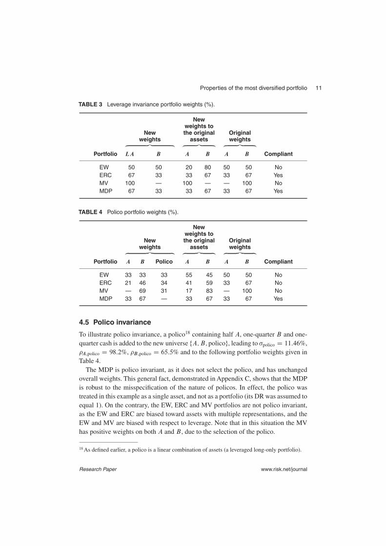
TABLE 3 Leverage invariance portfolio weights (%).
Newweights to
New the original Originalweights assets weights
‚ …„ ƒ ‚ …„ ƒ ‚ …„ ƒ
Portfolio LA B A B A B Compliant
EW 50 50 20 80 50 50 No
ERC 67 33 33 67 33 67 Yes
MV 100 — 100 — — 100 No
MDP 67 33 33 67 33 67 Yes
TABLE 4 Polico portfolio weights (%).
Newweights to
New the original Originalweights assets weights
‚ …„ ƒ ‚ …„ ƒ ‚ …„ ƒ
Portfolio A B Polico A B A B Compliant
EW 33 33 33 55 45 50 50 No
ERC 21 46 34 41 59 33 67 No
MV — 69 31 17 83 — 100 No
MDP 33 67 — 33 67 33 67 Yes
4.5 Polico invariance
To illustrate polico invariance, a polico18 containing half A, one-quarter B and one-
quarter cash is added to the new universe fA; B; policog, leading to �polico D 11:46%,
�A;polico D 98:2%, �B;polico D 65:5% and to the following portfolio weights given in
Table 4.
The MDP is polico invariant, as it does not select the polico, and has unchanged
overall weights. This general fact, demonstrated inAppendix C, shows that the MDP
is robust to the misspecification of the nature of policos. In effect, the polico was
treated in this example as a single asset, and not as a portfolio (its DR was assumed to
equal 1). On the contrary, the EW, ERC and MV portfolios are not polico invariant,
as the EW and ERC are biased toward assets with multiple representations, and the
EW and MV are biased with respect to leverage. Note that in this situation the MV
has positive weights on both A and B , due to the selection of the polico.
18As defined earlier, a polico is a linear combination of assets (a leveraged long-only portfolio).
Research Paper www.risk.net/journal
12 Y. Choueifaty et al
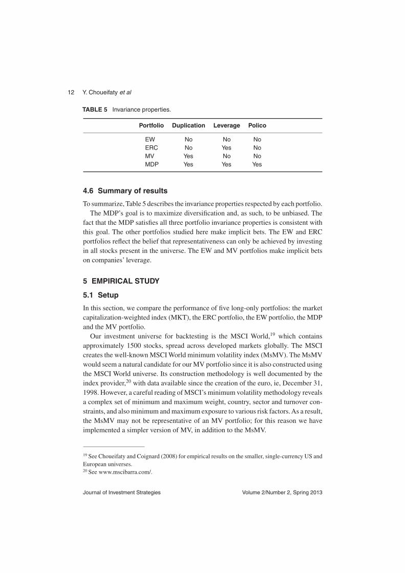
TABLE 5 Invariance properties.
Portfolio Duplication Leverage Polico
EW No No No
ERC No Yes No
MV Yes No No
MDP Yes Yes Yes
4.6 Summary of results
To summarize, Table 5 describes the invariance properties respected by each portfolio.
The MDP’s goal is to maximize diversification and, as such, to be unbiased. The
fact that the MDP satisfies all three portfolio invariance properties is consistent with
this goal. The other portfolios studied here make implicit bets. The EW and ERC
portfolios reflect the belief that representativeness can only be achieved by investing
in all stocks present in the universe. The EW and MV portfolios make implicit bets
on companies’ leverage.
5 EMPIRICAL STUDY
5.1 Setup
In this section, we compare the performance of five long-only portfolios: the market
capitalization-weighted index (MKT), the ERC portfolio, the EW portfolio, the MDP
and the MV portfolio.
Our investment universe for backtesting is the MSCI World,19 which contains
approximately 1500 stocks, spread across developed markets globally. The MSCI
creates the well-knownMSCIWorld minimum volatility index (MsMV). TheMsMV
would seem a natural candidate for our MV portfolio since it is also constructed using
the MSCI World universe. Its construction methodology is well documented by the
index provider,20 with data available since the creation of the euro, ie, December 31,
1998. However, a careful reading ofMSCI’s minimum volatility methodology reveals
a complex set of minimum and maximum weight, country, sector and turnover con-
straints, and alsominimum andmaximum exposure to various risk factors.As a result,
the MsMV may not be representative of an MV portfolio; for this reason we have
implemented a simpler version of MV, in addition to the MsMV.
19 See Choueifaty and Coignard (2008) for empirical results on the smaller, single-currency US and
European universes.20 See www.mscibarra.com/.
Journal of Investment Strategies Volume 2/Number 2, Spring 2013

Properties of the most diversified portfolio 13
The ERC, EW, MV and MDP portfolios were rebalanced semi-annually,21 and
stocks belonging to the MSCI index were selected at each rebalancing date. In order
to avoid liquidity and price availability issues in such a broad universe, we only
considered, at each rebalancing date, the top half of stocks by market capitalization22
(793 stocks on average, representing 90% of the index capitalization). To allow for
a fair comparison between our portfolios and MKT, we also built a synthetic market
cap-weighted index labeled MKT/2, comprised of the top half of stocks ranked by
market capitalization. For an appropriate comparison with the MsMV portfolio, we
simply added a maximum weight, a regional constraint, as well as a turnover penalty
to the MV and MDP construction.23
In order to use data reflecting as much recent information as possible, we estimated
the covariance matrices for the ERC, MV and MDP using a one-year window of past
daily returns,24 at each rebalancing date. To account for the impact of time zone
differences, we developed a “plesiochronous correlation estimator”,25 which allows
for the joint estimation of asset correlations, while taking into account the time delay
between observations.26 As having fewer observations than the number of assets
results in a nondefinite covariance matrix, we have also considered using a basic,
yet robust, method consisting of shrinking half of the correlation matrix towards the
21 Portfolios are rebalanced at the end of May and November, as is the MsMV.22At each rebalancing date, we eliminated all stocks with less than six months’ price history, and
selected the top half of the remaining stocks by market capitalization. Local currency total returns
were converted to USD, according to the MSCI methodology, and MSCI’s official forex data was
used. Total returns and market capitalization were obtained through Bloomberg.23 Having in mind MSCI’s methodology, we added a 1.5% maximum weight constraint, and a
maximum weight by time zone (America, Europe, Asia), to ensure allocation to the zones do not
exceed those of the MSCI World (MKT) by more than 5%. We also added a turnover reduction
penalty to the MDP and MV objective functions, such that the annualized tracking error to the
unpenalized problem was no greater than 1.5%. We did not add those constraints to the ERC
portfolio, as they were generally satisfied in its unconstrained version.24 Having fewer observations than the number of assets results in a nondefinite covariance matrix.
This was not an issue for the MDP and MV in the back tests presented here, as all portfolios
contained fewer assets than observations (159 on average for the MV and 137 for the MDP), and
were shown to be the unique solution of their optimization programs.25 Plesio means “near” in Greek, thus plesiochronous can be understood as “almost synchronous”.
We chose this term to represent the fact that even if the Japanese and US stock markets, for example,
never trade simultaneously, their time delay is mostly constant.26 This estimator was developed in spirit of the work done by Hayashi andYoshida (2005). See also
Hoffmann et al (2009) for further references.
Research Paper www.risk.net/journal

14 Y. Choueifaty et al
identity matrix.27 Portfolios built using these positive symmetric definite matrixes are
labeled ERCPSD, MDPPSD and MVPSD.
Finally, while it is straightforward to verify whether a portfolio has the ERC prop-
erty, a direct implementation of the numerical optimization algorithms, as proposed
in Maillard et al (2010), can require prohibitive computation time. For our purposes,
we chose to implement the optimization problem (7) of their paper, which provides a
unique, well-defined, long-only portfolio that respects the ERC property.28
5.2 Performance
The portfolios’ empirical performance is shown in Figure 1 on the facing page and
summarized in Table 6 on the facing page. All portfolios outperform MKT, which is
consistent with the documented inefficiency of market cap-weighted indexes, even
when assuming unrealistically high all-in trading costs of the order of 2%29 to account
for their higher turnover. The ERC, MV andMDP deliver significantly higher returns
and lower volatility, whereas the EW outperforms the market cap-weighted index
with comparable volatility. The ERC, in turn, functions as a risk-weighted version
of the EW, with marginally higher returns and significantly lower risk. Among the
portfolios with the lowest risk, the MsMV registers a modest performance advantage,
with significantly less volatility than the cap-weighted index. Its MV counterpart,
which has fewer constraints, has the lowest realized volatility, with returns similar in
magnitude to the ERC portfolio.
Table 7 on page 16 provides performance for the ERCPSD, MDPPSD and MVPSD
portfolios. Overall returns and volatilities are mostly unchanged30 compared with
original versions of these portfolios. However, using the shrinkage method lessens
turnover by 5 to 10%, with the MV and MDP portfolios holding 41 and 24 more
27 This method produces positive-definite matrices with eigenvalues greater than 0.5, and associated
covariance matrices that are also positive-definite. We choose a high, constant, shrinkage intensity
to ensure robustness. For references, see Ledoit and Wolf (2004).28 The solution is unique, provided of course that the covariance matrix is definite. We found that
with a standard PC (Intel Xeon at 2.66 GHz with 8 Gb of RAM), those optimizations required less
than a couple of seconds to converge, even when considering one thousand assets.29 Unrealistic all-in trading costs of 3.4% (respectively, 2.4%)would be needed for theMDP’s higher
turnover to be such that its outperformance relative to the market cap benchmark reduces to zero
(respectively, for both the EW and ERC).30 This may come as a surprise to practitioners used to long–short portfolio optimizations and
to observing drastically different (and improved) results. However, the MV and MDP portfolios
considered in this paper are long-only, and contain fewer assets than observations.As such, they are
much less sensitive to the estimation errors of the covariance matrix. Also, the long-only constraint
has already an effect similar to using a robust estimation technique (see Jagannathan and Ma 2003).
Journal of Investment Strategies Volume 2/Number 2, Spring 2013

Properties of the most diversified portfolio 15
FIGURE 1 Comparison of quantitative portfolio performances.
1998 1999 2000 2001 2002 2003 2004 2005 20072006 2008 2009 20100.7
1.0
1.3
1.6
1.9
2.2
2.5
Port
folio
pe
rfo
rma
nce
MDPERCMKT EW MV
TABLE 6 Comparison of quantitative portfolio performances, 1999–2010.
Statistic MKT MKT/2 MMV EW ERC MV MDP
Return 3.1% 2.9% 4.2% 5.8% 6.3% 6.7% 7.9%
Volatility (monthly) 16.6% 16.3% 11.7% 16.7% 13.1% 10.0% 11.4%
Volatility (daily) 17.2% 17.2% 12.3% 16.4% 12.9% 10.0% 11.2%
Turnover (one way) 14% 11% 23% 29% 50% 76% 82%
Tracking Error (daily) 0.0% 0.8% 7.6% 3.6% 6.7% 10.4% 9.2%
DR (daily) 2.3 2.2 2.8 2.5 3.0 3.4 3.7
nbStocks (avg) 1586 793 250 793 793 159 137
Sharpe (monthly) 0.00 0.01 0.05 0.16 0.24 0.36 0.42
Sharpe (daily) 0.00 0.01 0.06 0.16 0.24 0.36 0.43
stocks, respectively. This can be expected, as shrunken correlation matrices are by
design more stable over time, with the MV and MDP implicitly shrunk toward the
equal-variance-weighted and equal-volatility-weighted portfolios.
Research Paper www.risk.net/journal
16 Y. Choueifaty et al
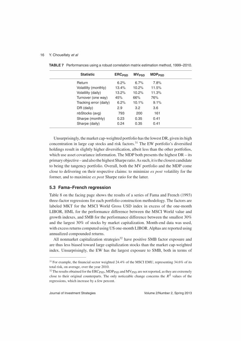
TABLE 7 Performances using a robust correlation matrix estimation method, 1999–2010.
Statistic ERCPSD MVPSD MDPPSD
Return 6.2% 6.7% 7.8%
Volatility (monthly) 13.4% 10.2% 11.5%
Volatility (daily) 13.2% 10.2% 11.3%
Turnover (one way) 45% 66% 76%
Tracking error (daily) 6.2% 10.1% 9.1%
DR (daily) 2.9 3.2 3.6
nbStocks (avg) 793 200 161
Sharpe (monthly) 0.23 0.35 0.41
Sharpe (daily) 0.24 0.35 0.41
Unsurprisingly, themarket cap-weighted portfolio has the lowest DR, given its high
concentration in large cap stocks and risk factors.31 The EW portfolio’s diversified
holdings result in slightly higher diversification, albeit less than the other portfolios,
which use asset covariance information. The MDP both presents the highest DR – its
primaryobjective – and also the highest Sharpe ratio.As such, it is the closest candidate
to being the tangency portfolio. Overall, both the MV portfolio and the MDP come
close to delivering on their respective claims: to minimize ex post volatility for the
former, and to maximize ex post Sharpe ratio for the latter.
5.3 Fama–French regression
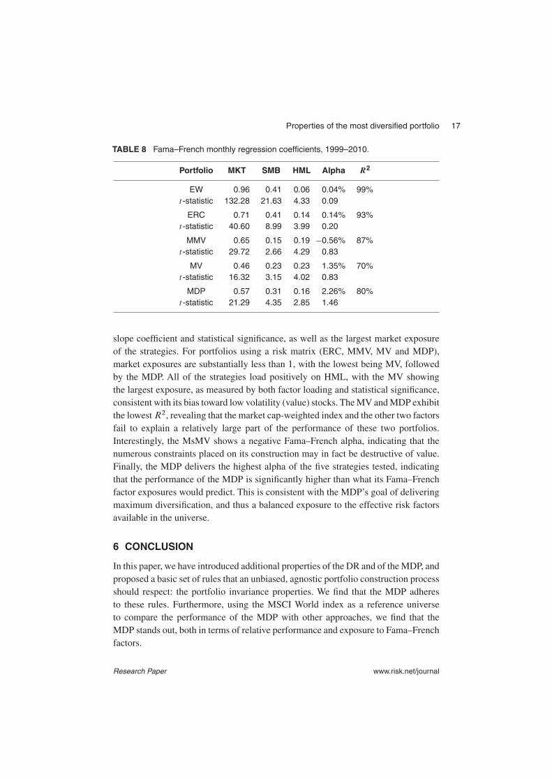
Table 8 on the facing page shows the results of a series of Fama and French (1993)
three-factor regressions for each portfolio construction methodology. The factors are
labeled MKT for the MSCI World Gross USD index in excess of the one-month
LIBOR, HML for the performance difference between the MSCI World value and
growth indexes, and SMB for the performance difference between the smallest 30%
and the largest 30% of stocks by market capitalization. Month-end data was used,
with excess returns computed using US one-month LIBOR.Alphas are reported using
annualized compounded returns.
All nonmarket capitalization strategies32 have positive SMB factor exposure and
are thus less biased toward large capitalization stocks than the market cap-weighted
index. Unsurprisingly, the EW has the largest exposure to SMB, both in terms of
31 For example, the financial sector weighted 24.4% of the MSCI EMU, representing 34.6% of its
total risk, on average, over the year 2010.32 The results obtained for the ERCPSD, MDPPSD andMVPSD are not reported, as they are extremely
close to their original counterparts. The only noticeable change concerns the R2 values of the
regressions, which increase by a few percent.
Journal of Investment Strategies Volume 2/Number 2, Spring 2013
Properties of the most diversified portfolio 17
TABLE 8 Fama–French monthly regression coefficients, 1999–2010.
Portfolio MKT SMB HML Alpha R2
EW 0.96 0.41 0.06 0.04% 99%
t -statistic 132.28 21.63 4.33 0.09
ERC 0.71 0.41 0.14 0.14% 93%
t -statistic 40.60 8.99 3.99 0.20
MMV 0.65 0.15 0.19 0.56% 87%
t -statistic 29.72 2.66 4.29 0.83
MV 0.46 0.23 0.23 1.35% 70%
t -statistic 16.32 3.15 4.02 0.83
MDP 0.57 0.31 0.16 2.26% 80%
t -statistic 21.29 4.35 2.85 1.46
slope coefficient and statistical significance, as well as the largest market exposure
of the strategies. For portfolios using a risk matrix (ERC, MMV, MV and MDP),
market exposures are substantially less than 1, with the lowest being MV, followed
by the MDP. All of the strategies load positively on HML, with the MV showing
the largest exposure, as measured by both factor loading and statistical significance,
consistent with its bias toward low volatility (value) stocks. TheMV andMDP exhibit
the lowest R2, revealing that the market cap-weighted index and the other two factors
fail to explain a relatively large part of the performance of these two portfolios.
Interestingly, the MsMV shows a negative Fama–French alpha, indicating that the
numerous constraints placed on its construction may in fact be destructive of value.
Finally, the MDP delivers the highest alpha of the five strategies tested, indicating
that the performance of the MDP is significantly higher than what its Fama–French
factor exposures would predict. This is consistent with the MDP’s goal of delivering
maximum diversification, and thus a balanced exposure to the effective risk factors
available in the universe.
6 CONCLUSION
In this paper, we have introduced additional properties of the DR and of theMDP, and
proposed a basic set of rules that an unbiased, agnostic portfolio construction process
should respect: the portfolio invariance properties. We find that the MDP adheres
to these rules. Furthermore, using the MSCI World index as a reference universe
to compare the performance of the MDP with other approaches, we find that the
MDP stands out, both in terms of relative performance and exposure to Fama–French
factors.
Research Paper www.risk.net/journal
18 Y. Choueifaty et al
Classical financial theory defines the equity risk premium as the return of the
undiversifiable portfolio. In developing the MDP, our goal was to articulate a theory
and a consistent construction methodology that deliver the full benefit of the equity
risk premium to investors and their trustees, and we believe that our work shows that
the MDP is a strong candidate for being the undiversifiable portfolio.
APPENDIX A
A.1 Notation
In the following, we denote byˇ the element-wise product of two vectors and by˛the element-wise division of two vectors.
A.2 Diversification ratio decomposition
Noting Qw D wˇ � , the variance of the portfolio with weights w can be written as
�2.w/ DX
i
Qw2i C 2
X
i<j
Qwi Qwj �i;j DX
i
Qw2i C �.w/
X
i¤j
Qwi Qwj :
Noting that
X
i¤j
Qwi Qwj D�
X
i
Qwi
�2
X
i
Qw2i
leads to
�2.w/ D .1 �. Qw//X
i
Qw2i C �.w/
�X
i
Qwi
�2
:
Then, dividing this equality by .P
i Qwi /2 gives the decomposition
1
DR.w/2D .1 �.w//CR.w/C �.w/:
APPENDIX B
B.1 Most diversified portfolios’ existence and uniqueness
The MDP optimization is a quadratic programming problem on a convex set: thanks
to the fact that the DR is invariant by scalar multiplication, this is equivalent to
minw12w0˙w, constrained by wi > 0 and
P
i wi�i D 1, with weights rescaled to
sum to 1 afterwards. The existence follows; uniqueness also follows if the covariance
matrix is definite (see Berkovitz 2001, pp. 210–215).
Journal of Investment Strategies Volume 2/Number 2, Spring 2013
Properties of the most diversified portfolio 19
B.2 Most diversified portfolios’ first-order conditions
Wefirst apply theKarush–Kuhn–Tucker (KKT) theorem: all admissible points qualify,
according to the linear independence constraint qualification (equality and inequality
are independent unless all the inequality constraints are active, which would mean
that w D 0). The log of our positive objective function is
f .w/ D ln.DR.w// D lnh� j wi 12lnh˙w j wi;
with
rfw D1
h� j wi� 1
2
1
h˙w j wi2˙w:
The KKT theorem states that at optimal points w�, there exist a vector � 2 R
N and
a scalar � such that
1
h� j w�i� 1
�.w�/2˙w
� C �1C � D 0;
min.�; w�/ D 0;
hw� j 1i D 1:
Multiplying the first condition on the left by the transpose of w�, shows that � must
be 0, and that the first condition is independent of the constraint that weights sum to
1. This does not come as a surprise, as the DR is invariant by scalar multiplication.
Define � D �2.w�/�; an optimal point w� is necessarily associated to a vector
� 2 RN satisfying
˙w� D �.w�/2
h� j w�i� C �;
min.�; w�/ D 0;
hw� j 1i D 1:
B.3 The core property of the most diversified portfolio (2)
Wefirst show that theMDP respects the core property (2).Bydefinition, the correlation
of the MDP to any other portfolio reads
�w;wMDP D h˙wMDP j wi
�.wMDP/�.w/:
Research Paper www.risk.net/journal
20 Y. Choueifaty et al
Given that
˙wMDP D ı� C �; with ı D �.wMDP/
DR.wMDP/;
we have
�w;wMDP D 1
DR.wMDP/�.w/
�
� C 1
ı�
ˇˇˇˇ
w
�
:
Keeping in mind that � is nonnegative, for all long-only portfolios with nonnegative
weights w,
�w;wMDP >1
DR.wMDP/�.w/h� j wi;
which leads us to the final result. We now prove that a portfolio w� that respects the
core property (2) necessarily maximizes the DR.As w� respects the property (2), we
have, for all long-only portfolios, �w;w� > DR.w/=DR.w�/. Since correlations are
not greater than unity, for all long-only portfolios we have DR.w�/ > DR.w/, which
shows that w� maximizes the DR across all long-only portfolios.
B.4 The core property of the most diversified portfolio (1)
Suppose that the MDP satisfies the core property (2). For any asset belonging to
the MDP, the inequality given by the core property (2) becomes an equality as
min.�; wMDP/ D 0. Since the DR of a single asset equals 1, we have, for any given
asset in the MDP,
�in;wMDP D 1
DR.wMDP/:
Now, using the core property (2) for any stock outside of the MDP, we finally obtain
�out;wMDP >1
DR.wMDP/D �in;wMDP :
Thus, the MDP satisfies the core property (1).
Conversely, suppose that a portfolio w� satisfies the core property (1), for a given
correlation �in;w� . Then, for any long-only portfolio w:
�w;w� D wT.˙w
�/
�.w/�.w�/D 1
�.w/�.w�/
X
iD1;:::;N
wi�i�.w�/�i;w�
> �in;w�
P
iD1;:::;N wi�i
�.w/D �in;w�DR.w/:
Applied with w D w�, we have an equality. This shows that �in;w�DR.w�/ D 1, and
DR.w/ 6 �w;w�DR.w�/ 6 DR.w�/. This demonstrates that w� is the MDP, as it
Journal of Investment Strategies Volume 2/Number 2, Spring 2013
Properties of the most diversified portfolio 21
has maximum diversification across all long-only portfolios. Overall, this shows that
the core property of the MDP (1) is equivalent to the core property of the MDP (2).
B.5 Correlation of assets to the unconstrained most diversified
portfolio
When removing the long-only constraint � for all portfolios, possibly long–short,
�w;wMDP D DR.w/
DR.wMDP/:
In particular, the correlations of all assets to the MDP are constant, and equal to the
inverse of the MDP’s DR.
APPENDIX C
C.1 The most diversified portfolio is leverage invariant
The first-order condition for the MDP can be rewritten by splitting the covariance
matrix into volatilities and correlations:
� ˇ C.� ˇw/ D ı� C �:
Asvolatilities are positive, this is equivalent toC.�ˇw/ D ı1C�0withmin.�0; w/ D
0 and �0 D �˛ � . Now, applying a positive leverage vector L D .Li /iD1;:::;A, the
leveraged assets have the same correlation matrix C and volatilities �L D .Li�i /.
The portfolio wL D kw˛L is the MDP in the leveraged universe (with k a positive
normalization constant, such that hw j 1i D 1), as it verifies the first-order condition
C.� L ˇwL/ D kı1C k�
0 with min.k�0; w
L/ D 0. This means that �L ˇw
L Dk� ˇw. Thus, the leverage invariance property is proved.
C.2 The most diversified portfolio is polico invariant
The core property of the MDP (2) shows that the MDP is such that any asset not
selected by the MDP has a correlation greater than 1=DR.MDP/. This means the
MDP is unchanged by adding to the universe any asset with a correlation strictly
greater than 1=DR.MDP/. Furthermore, if we consider any polico �, we have
�.�;MDP/ >DR.�/
DR.MDP/>
1
DR.MDP/;
as the DR of a polico is greater than 1. This means that when the polico is added to
the universe, it is never selected, and the MDP remains unchanged (otherwise, we
would have had �.�;MDP/ D 1=DR.MDP/ according to the core property (2)).
Research Paper www.risk.net/journal
22 Y. Choueifaty et al
REFERENCES
Arnott, R., Hsu, J., and Moore, P. (2005). Fundamental indexation. Financial Analysts Jour-
nal 61(2), 83–99.
Arnott, R., Kalesnik, V., Moghtader P., and Scholl, C. (2010). Beyond cap weight. Journal
of Indexes 16(1), 16–29.
Berkovitz, L. D. (2001). Convexity and Optimization in Rn. Wiley.
Bouchaud, J. P., and Potters, M. (2009). Theory of Financial Risk and Derivative Pricing.
Cambridge University Press.
Choueifaty, Y. (2006). Methods and systems for providing an anti-benchmark portfolio.
USPTO 60/816, 276.
Choueifaty,Y., and Coignard,Y. (2008).Toward maximum diversification.Journal of Portfolio
Management 35(1), 40–51.
Chow, T., Hsu, J., Kalesnik, V., and Little, B. (2011). A survey of alternative equity index
strategies. Financial Analysts Journal 67(5), 37–57.
Clarke, R., de Silva, H., and Thorley, S. (2006). Minimum-variance portfolios in the US
equity market. Journal of Portfolio Management 33(1), 10–24.
Fama, E. F., and French, K. R. (1993). Common risk factors in the returns on stocks and
bonds. Journal of Financial Economics 33, 3–56.
Haugen, R. A., and Baker, N. (1991). The efficient market inefficiency of capitalization-
weighted stock portfolios. Journal of Portfolio Management 17(3), 35–40.
Haugen, R. A., and Heins, A. J. (1975). Risk and the rate of return on financial assets: some
old wine in new bottles. Journal of Financial and Quantitative Analysis 10(5), 775–784.
Hayashi, T., and Yoshida, N. (2005). On covariance estimation of non-synchronously
observed diffusion processes. Bernoulli 11(2), 359–379.
Hoffmann, M., Rosenbaum, M., and Yoshida, N. (2009). Estimation of the lead-lag param-
eter from non-synchronous data. Working Paper, CREST.
Jagannathan, R., and Ma, T. (2003). Risk reduction in large portfolios: why imposing the
wrong constraints helps. Journal of Finance 58(4), 1651–1684.
Ledoit, O., and Wolf, M. (2004). A well-conditioned estimator for large-dimensional covari-
ance matrices. Journal of Multivariate Analysis 88(2), 365–411.
Maillard, S., Roncalli, T., and Teiletche, J. (2010). The properties of equally weighted risk
contribution portfolio. Journal of Portfolio Management 36(4), 60–70.
Markowitz, H. M. (1952). Portfolio selection. Journal of Finance 7(1), 77–91.
Rhoades, S. A. (1993). The Herfindahl–Hirschman index. Federal Reserve Bulletin 38(1),
188–189.
Sharpe, W. (1991). Capital asset prices with and without negative holdings. Journal of
Finance 46(2), 489–509.
Journal of Investment Strategies Volume 2/Number 2, Spring 2013