03 - lte dimensioning guidelines - outdoor link budget - fdd - ed2.9 - internal (1)
DESCRIPTION
LTE Dimensioning Guidelines - Outdoor Link BudgetTRANSCRIPT
INTERNAL
LTE Dimensioning Guidelines – Outdoor Link Budget - FDD
February 2011
< LTE DIMENSIONING GUIDELINES – OUTDOOR LINK BUDGET> <FEB.2011>
Alcatel-Lucent – Proprietary
Version 2.9 2 / 61
INTERNAL
Copyright © 2011 by Alcatel-Lucent. All Rights Reserved.
About Alcatel-Lucent
Alcatel-Lucent (Euronext Paris and NYSE: ALU) provides solutions that enable service
providers, enterprises and governments worldwide, to deliver voice, data and video
communication services to end-users. As a leader in fixed, mobile and converged broadband
networking, IP technologies, applications, and services, Alcatel-Lucent offers the end-to-
end solutions that enable compelling communications services for people at home, at work
and on the move. For more information, visit Alcatel-Lucent on the Internet.
Notice
The information contained in this document is subject to change without notice. At the
time of publication, it reflects the latest information on Alcatel-Lucent’s offer, however,
our policy of continuing development may result in improvement or change to the
specifications described.
Trademarks
Alcatel, Lucent Technologies, Alcatel-Lucent and the Alcatel-Lucent logo are trademarks of
Alcatel-Lucent. All other trademarks are the property of their respective owners. Alcatel-
Lucent assumes no responsibility for inaccuracies contained herein.
< LTE DIMENSIONING GUIDELINES – OUTDOOR LINK BUDGET> <FEB.2011>
Alcatel-Lucent – Proprietary
Version 2.9 3 / 61
INTERNAL
History
Changes Date Author
Ed 1.0 – 1st Release Dec 2008 Keith Butterworth
Ed 2.0 - Quality review and edits, minor edits to section 4.1 Feb 2009 Keith Butterworth
Ed2.1 – Correction to interference margin definition Mar 2009 Keith Butterworth
Ed2.2 – Updates to modem performances and active user &
throughput computations. Revamp of parameter naming for air
interface and modem computations. Addition of ACK/NACK link
budget considerations.
Jun 2009 Keith Butterworth
Ed2.3 – Updates to the link budget aspects (modification of UL
link budget + addition of revised DL link budget). Nov 2009 Keith Butterworth
Ed2.3 – Minor updates and corrections Dec 2009 Keith Butterworth
Ed2.5 – Alignment with Ed8.2 link budget (updated SINR
figures, FSS Gain, revised IoT section, rework of DL section,
spatial multiplexing gain)
Feb 2010 Keith Butterworth
Ed2.6 – Update inline with new dimensioning guidelines
document structure + alignment with changes in Ed8.3.2 of link
budget tool
Apr 2010 Keith Butterworth
Ed2.7 – Minor changes to sections 2.1.4.4, 3.1.3 and 3.1.5.4. Jul 2010 Keith Butterworth
Ed2.8 – Minor editorial updates (correction of interference
margin equation). Updates to align with Ed 8.4 of the LKB tool.
Addition of 8bit CQI report over PUCCH link budget.
Sept 2010 Keith Butterworth
Ed2.9 – Updates to align with Ed8.5 of the LKB tool. Correction
of effective coding rates and other minor corrections. Feb 2011 Laurent Demerville
Reviewed by ARFCC (Advanced RF Competence Centre)
< LTE DIMENSIONING GUIDELINES – OUTDOOR LINK BUDGET> <FEB.2011>
Alcatel-Lucent – Proprietary
Version 2.9 4 / 61
INTERNAL
CONTENTS
1 Introduction ....................................................................... 8
2 Uplink Link Budget..............................................................10
2.1 Uplink Link Budget Parameters................................................. 11 2.1.1 UE Characteristics......................................................................12 2.1.2 eNode-B Receiver Sensitivity.........................................................12 2.1.3 Noise Figure.............................................................................12 2.1.4 SINR Performances .....................................................................13 2.1.5 Handling of VoIP on the Uplink ......................................................21 2.1.6 Uplink Explicit Diversity Gains .......................................................23 2.1.7 Interference Margin....................................................................24 2.1.8 Shadowing Margin ......................................................................27 2.1.9 Handoff Gain / Best Server Selection Gain ........................................28 2.1.10 Frequency Selective Scheduling (FSS) Gain ........................................30 2.1.11 Penetration Losses .....................................................................32
2.2 Final MAPL and Cell Range....................................................... 32 2.2.1 Propagation Model .....................................................................33 2.2.2 Site Area.................................................................................34
2.3 Impact of RRH and TMA .......................................................... 35 2.3.1 RRH .......................................................................................35 2.3.2 TMA.......................................................................................35
2.4 Uplink Budget Example........................................................... 36
2.5 Uplink Common Control Channel Considerations ........................... 36 2.5.1 Attach Procedure.......................................................................37 2.5.2 ACK/NACK Feedback...................................................................38 2.5.3 Periodic CQI Reports...................................................................40
3 Downlink Link Budget ..........................................................42
3.1 Downlink Budget Parameters ................................................... 43 3.1.1 SINR.......................................................................................43 3.1.2 RSRQ......................................................................................45 3.1.3 Interference Sources ..................................................................46 3.1.4 Geometry................................................................................47 3.1.5 Downlink SINR Performances .........................................................50 3.1.6 Resource Element Distribution.......................................................54 3.1.7 Energy Per Resource Element (EPRE) ...............................................55 3.1.8 Shadowing Margin & Handoff Gain ..................................................56
3.2 Downlink Budget Example ....................................................... 57
4 Downlink Output Power........................................................59
5 Radio Network Planning .......................................................60
6 Summary ..........................................................................61
< LTE DIMENSIONING GUIDELINES – OUTDOOR LINK BUDGET> <FEB.2011>
Alcatel-Lucent – Proprietary
Version 2.9 5 / 61
INTERNAL
EXECUTIVE SUMMARY
The purpose of this series of dimensioning guidelines is to describe details of Alcatel-
Lucent’s dimensioning rules for the LTE Frequency Division Duplex (FDD) air interface and
eNode-B modem hardware.
A first step of the network design process consists of determining the number of sites
required and deployment feasibility according to the following information:
� Site density of any legacy network deployments,
� Frequency band(s) used by the legacy system(s), if applicable
� Frequency band(s) used by the LTE system,
� Bandwidth available for LTE (1.4, 3, 5, 10, 15 or 20 MHz),
� Requirements in terms of LTE data rates at cell edge (e.g. uplink data edge to be
guaranteed, best effort data, VoIP coverage requirements, etc.).
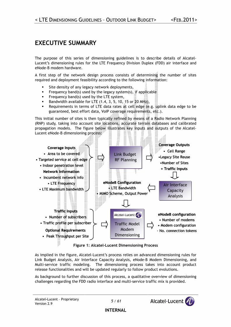
This initial number of sites is then typically refined by means of a Radio Network Planning
(RNP) study, taking into account site locations, accurate terrain databases and calibrated
propagation models. The figure below illustrates key inputs and outputs of the Alcatel-
Lucent eNode-B dimensioning process:
Coverage Inputs
• Area to be covered
• Targeted service at cell edge
• Indoor penetration level
Traffic Inputs
• Number of subscribers
• Traffic profile per subscriber
Network Information
• Incumbent network info
• LTE Frequency
• LTE Maximum bandwidth
eNodeB Configuration
• LTE Bandwidth
• MIMO Scheme, Output Power
Coverage Outputs
• Cell Range
•Legacy Site Reuse
•Number of Sites
+ Traffic Inputs
Link Budget
RF Planning
Air Interface
Capacity
Analysis
Traffic Model
Modem
Dimensioning
Traffic Model
Modem
DimensioningOptional Requirements
• Peak Throughput per Site
eNodeB configuration
• Number of modems
• Modem configuration
- No. connection tokens
- UL & DL Throughput tokens
Figure 1: Alcatel-Lucent Dimensioning Process
As implied in the figure, Alcatel-Lucent’s process relies on advanced dimensioning rules for
Link Budget Analysis, Air Interface Capacity Analysis, eNode-B Modem Dimensioning, and
Multi-service traffic modeling. The dimensioning process takes into account product
release functionalities and will be updated regularly to follow product evolutions.
As background to further discussion of this process, a qualitative overview of dimensioning
challenges regarding the FDD radio interface and multi-service traffic mix is provided.
< LTE DIMENSIONING GUIDELINES – OUTDOOR LINK BUDGET> <FEB.2011>
Alcatel-Lucent – Proprietary
Version 2.9 6 / 61
INTERNAL
Internal: These rules are implemented in the dedicated LTE tools used by Network
Designers: “Alcatel-Lucent LTE Link Budget” for FDD and TDD link budget analysis, “9955
and ACCO” for radio network planning studies and “LTE eNode-B Dimensioning Tool” for air
interface capacity and modem dimensioning.
< LTE DIMENSIONING GUIDELINES – OUTDOOR LINK BUDGET> <FEB.2011>
Alcatel-Lucent – Proprietary
Version 2.9 7 / 61
INTERNAL
References
[1] Jakes W.C., “ Microwave Mobile Communications”, IEEE Press, 1994
[2] K.M Rege, S. Nanda, C.F. Weaver, W.C. Peng, “ Analysis of Fade Margins for Soft
and Hard Handoffs”, PIMRC, 1996
[3] K.M Rege, S. Nanda, C.F. Weaver, W.C. Peng, “Fade margins for soft and hard
handoffs”, Wireless Networks 2, 1996
< LTE DIMENSIONING GUIDELINES – OUTDOOR LINK BUDGET> <FEB.2011>
Alcatel-Lucent – Proprietary
Version 2.9 8 / 61
INTERNAL
1 INTRODUCTION
This document forms one part of a series of network dimensioning guidelines, as detailed in
Table 1.
Table 1: Design Topics Covered in the LTE Dimensioning Guidelines Package
Design Topic Document
Deployment Strategy LTE Dimensioning Guidelines - Deployment Strategy
Radio Features LTE Dimensioning Guidelines – Radio Features
Outdoor Link Budget LTE Dimensioning Guidelines – Outdoor Link Budget
Indoor Link Budget LTE Dimensioning Guidelines – Indoor Link Budget
Peak Throughput LTE Dimensioning Guidelines – Peak Throughput
Radio Network Planning LTE Dimensioning Guidelines – RNP
Air Interface Capacity LTE Dimensioning Guidelines – Air Interface Capacity
eNode-B Dimensioning LTE Dimensioning Guidelines – Modem
Token & Licensing Dimensioning LTE Dimensioning Guidelines – Token & Licensing
S1/X2 Dimensioning LTE Dimensioning Guidelines – S1 & X2
Frequency Reuse Considerations LTE Dimensioning Guidelines – Frequency Reuse
Diversity & MIMO LTE Dimensioning Guidelines – Diversity & MIMO
Traffic Power Control LTE Dimensioning Guidelines – Power Control
Traffic Aggregation Modeling LTE Dimensioning Guidelines – Traffic Aggregation Modeling
The purpose of this document is to detail the formulation of Alcatel-Lucent’s LTE link
budget for outdoor macro cellular deployments.
Link budgets are used by Alcatel-Lucent primarily to derive the expected LTE performances
at cell edge on the uplink and compare them with legacy systems in the case of an overlay
of an existing network. This enables the estimation of the proportion of sites that can be
reused (additional constraints such as space for hardware deployment, etc, have to be
considered on top of this) and/or the required number of sites for a Greenfield operator.
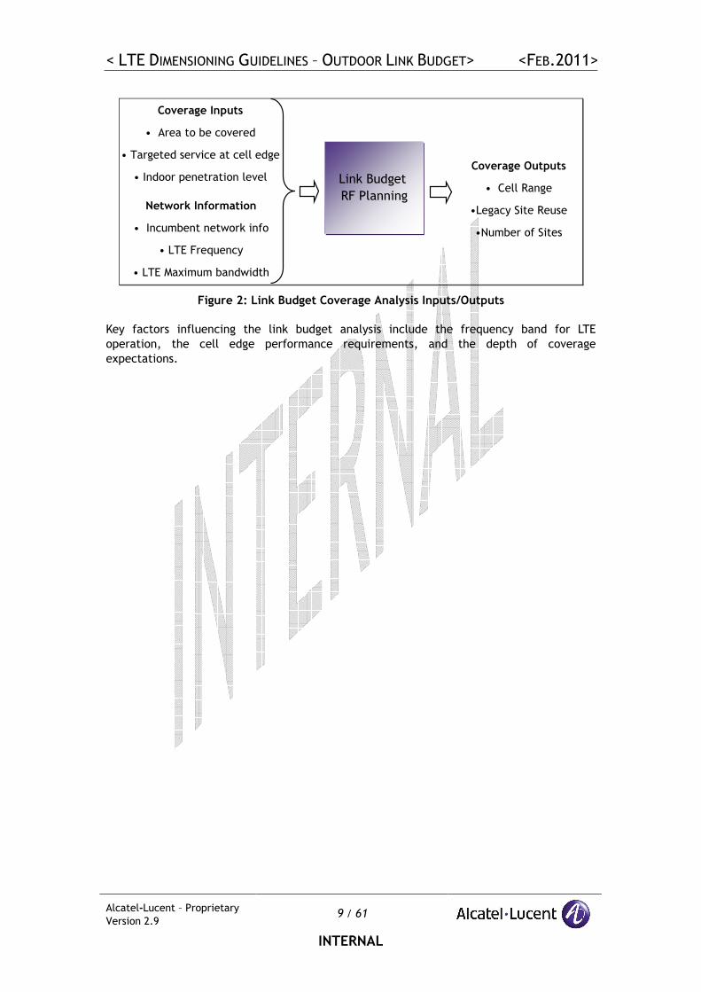
Figure 2 illustrates the main inputs and outputs for an LTE link budget coverage analysis.
< LTE DIMENSIONING GUIDELINES – OUTDOOR LINK BUDGET> <FEB.2011>
Alcatel-Lucent – Proprietary
Version 2.9 9 / 61
INTERNAL
Coverage Inputs
• Area to be covered
• Targeted service at cell edge
• Indoor penetration level
Network Information
• Incumbent network info
• LTE Frequency
• LTE Maximum bandwidth
Coverage Outputs
• Cell Range
•Legacy Site Reuse
•Number of Sites
Link Budget
RF Planning
Figure 2: Link Budget Coverage Analysis Inputs/Outputs
Key factors influencing the link budget analysis include the frequency band for LTE
operation, the cell edge performance requirements, and the depth of coverage
expectations.
< LTE DIMENSIONING GUIDELINES – OUTDOOR LINK BUDGET> <FEB.2011>
Alcatel-Lucent – Proprietary
Version 2.9 10 / 61
INTERNAL
2 UPLINK LINK BUDGET
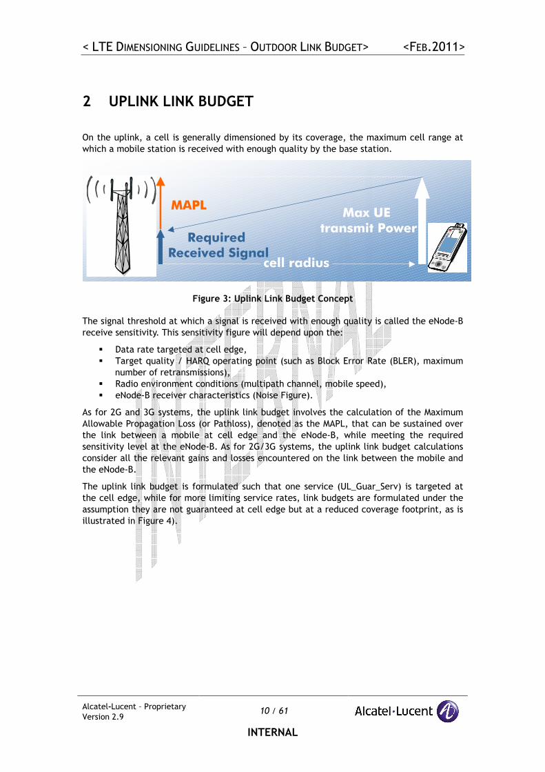
On the uplink, a cell is generally dimensioned by its coverage, the maximum cell range at
which a mobile station is received with enough quality by the base station.
cell radius
MAPL
Required Received Signal
Max UE transmit Power
Figure 3: Uplink Link Budget Concept
The signal threshold at which a signal is received with enough quality is called the eNode-B
receive sensitivity. This sensitivity figure will depend upon the:
� Data rate targeted at cell edge,
� Target quality / HARQ operating point (such as Block Error Rate (BLER), maximum
number of retransmissions),
� Radio environment conditions (multipath channel, mobile speed),
� eNode-B receiver characteristics (Noise Figure).
As for 2G and 3G systems, the uplink link budget involves the calculation of the Maximum
Allowable Propagation Loss (or Pathloss), denoted as the MAPL, that can be sustained over
the link between a mobile at cell edge and the eNode-B, while meeting the required
sensitivity level at the eNode-B. As for 2G/3G systems, the uplink link budget calculations
consider all the relevant gains and losses encountered on the link between the mobile and
the eNode-B.
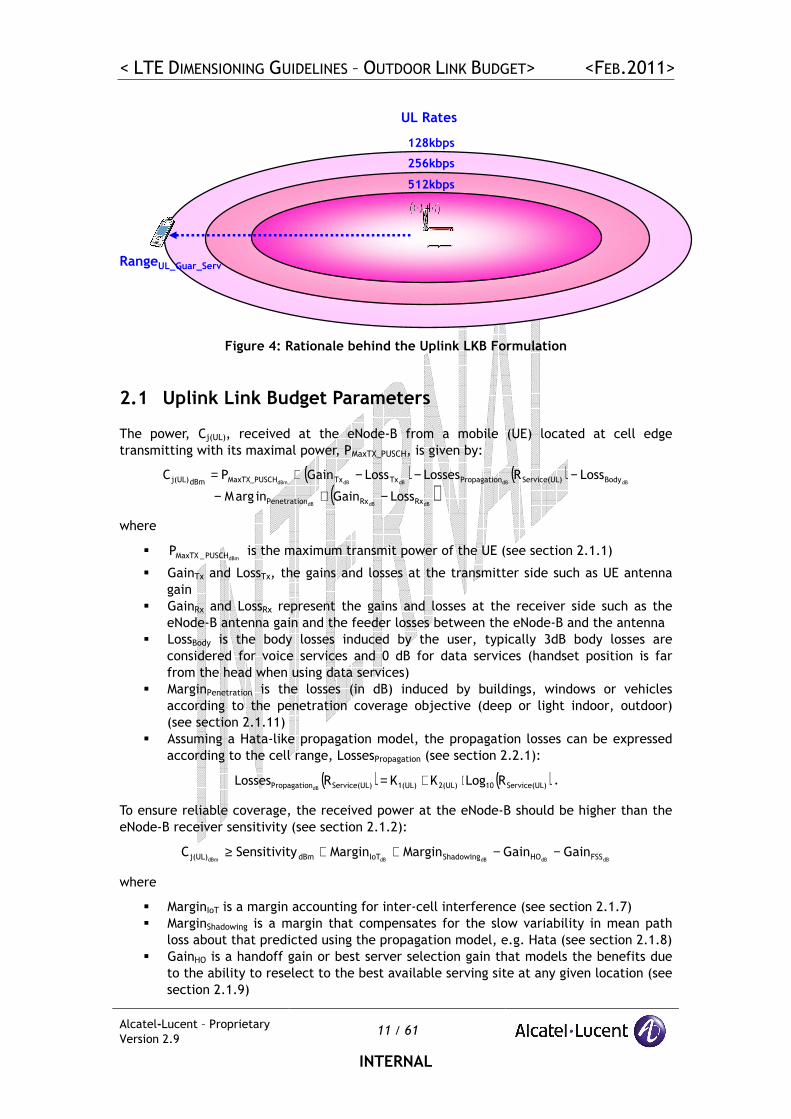
The uplink link budget is formulated such that one service (UL_Guar_Serv) is targeted at
the cell edge, while for more limiting service rates, link budgets are formulated under the
assumption they are not guaranteed at cell edge but at a reduced coverage footprint, as is
illustrated in Figure 4).
< LTE DIMENSIONING GUIDELINES – OUTDOOR LINK BUDGET> <FEB.2011>
Alcatel-Lucent – Proprietary
Version 2.9 11 / 61
INTERNAL
RangeUL_Guar_Serv
128kbps
256kbps
512kbps
UL Rates
Figure 4: Rationale behind the Uplink LKB Formulation
2.1 Uplink Link Budget Parameters
The power, Cj(UL), received at the eNode-B from a mobile (UE) located at cell edge
transmitting with its maximal power, PMaxTX_PUSCH, is given by:
( ) ( )( )
dBdBdB
dBdBdBdBdBm
RxRxnPenetratio
Body)Service(ULnPropagatioTxTxHMaxTX_PUSCdBmj(UL)
LossGaininargM
LossRLossesLossGainPC
−+−
−−−+=
where
� dBmPUSCH_MaxTXP is the maximum transmit power of the UE (see section 2.1.1)
� GainTx and LossTx, the gains and losses at the transmitter side such as UE antenna
gain
� GainRx and LossRx represent the gains and losses at the receiver side such as the
eNode-B antenna gain and the feeder losses between the eNode-B and the antenna
� LossBody is the body losses induced by the user, typically 3dB body losses are
considered for voice services and 0 dB for data services (handset position is far
from the head when using data services)
� MarginPenetration is the losses (in dB) induced by buildings, windows or vehicles
according to the penetration coverage objective (deep or light indoor, outdoor)
(see section 2.1.11)
� Assuming a Hata-like propagation model, the propagation losses can be expressed
according to the cell range, LossesPropagation (see section 2.2.1):
( ) ( ))Service(UL102(UL)1(UL))Service(ULnPropagatio RLogKKRLossesdB
⋅+= .
To ensure reliable coverage, the received power at the eNode-B should be higher than the
eNode-B receiver sensitivity (see section 2.1.2):
dBdBdBdBdBm FSSHOShadowingIoTdBmj(UL) GainGainMarginMarginySensitivitC −−++≥
where
� MarginIoT is a margin accounting for inter-cell interference (see section 2.1.7)
� MarginShadowing is a margin that compensates for the slow variability in mean path
loss about that predicted using the propagation model, e.g. Hata (see section 2.1.8)
� GainHO is a handoff gain or best server selection gain that models the benefits due
to the ability to reselect to the best available serving site at any given location (see
section 2.1.9)
< LTE DIMENSIONING GUIDELINES – OUTDOOR LINK BUDGET> <FEB.2011>
Alcatel-Lucent – Proprietary
Version 2.9 12 / 61
INTERNAL
� GainFSS is a frequency selective scheduling gain that is due to the ability of the
scheduler to select best frequency blocks per UE depending on their channel
conditions
For each service to be offered by the operator, this relationship allows computation of the
maximum propagation losses that can be afforded by a mobile located at the cell edge,
that is to say the Maximum Allowable Path Loss (MAPL):
dBdBdB
dBdB
dBdBdBdBdBdBm
FSSHOShadowing
IoTdBmnPenetratio
BodyRxRxTxTxHMaxTX_PUSCdBj(UL)
GainGainMargin
MarginySensitivitinargM
LossossLGainossLGainPMAPL
++−
−−−
−−+−+=
2.1.1 UE Characteristics
The maximum transmit power of an LTE UE, PMaxTX_PUSCH, depends on the power class of the
UE. Currently, only one power class is defined in 3GPP TS 36.101:
� A 23dBm output power is considered with a 0 dBi antenna gain.
Internal: This is the case in the TS 36.101 version of January 2011. Only one class defined
(Class 3) with 23dBm output power (with ±2dB tolerance, but we should not account for
such a tolerance to define the UE output power).
2.1.2 eNode-B Receiver Sensitivity
The sensitivity level can be derived from SINR figures calculated or measured for some
given radio channel conditions (multipath channel, mobile speed) and quality target (e.g.
10-2 BLER):
( )RBRB(UL)theNode_B10PUSCH_dBdBm .W.N.NFLog10 SINRySensitivit ⋅+=
where:
� SINRPUSCH_dB is the signal to interference ratio per Resource Block, required to reach
a given PUSCH data rate and quality of service,
� FeNode-B.Nth.NRB(UL).WRB is the total thermal noise level seen at the eNode-B receiver
within the required bandwidth to reach the given data rate, where:
� FeNode-B is the noise figure of the eNode-B receiver,
� Nth is the thermal noise density (-174dBm/Hz),
� NRB(UL) is the number of resource blocks (RB) required to reach a given data rate – it
can be deduced from link level simulations selecting the best combination (e.g. the
one that requires lowest SNR or lowest number of RB to maximize the capacity),
� WRB is the bandwidth used by one LTE Resource Block. One Resource Block is
composed of 12 subcarriers, each of a 15kHz bandwidth – so WRB is equal to 180kHz.
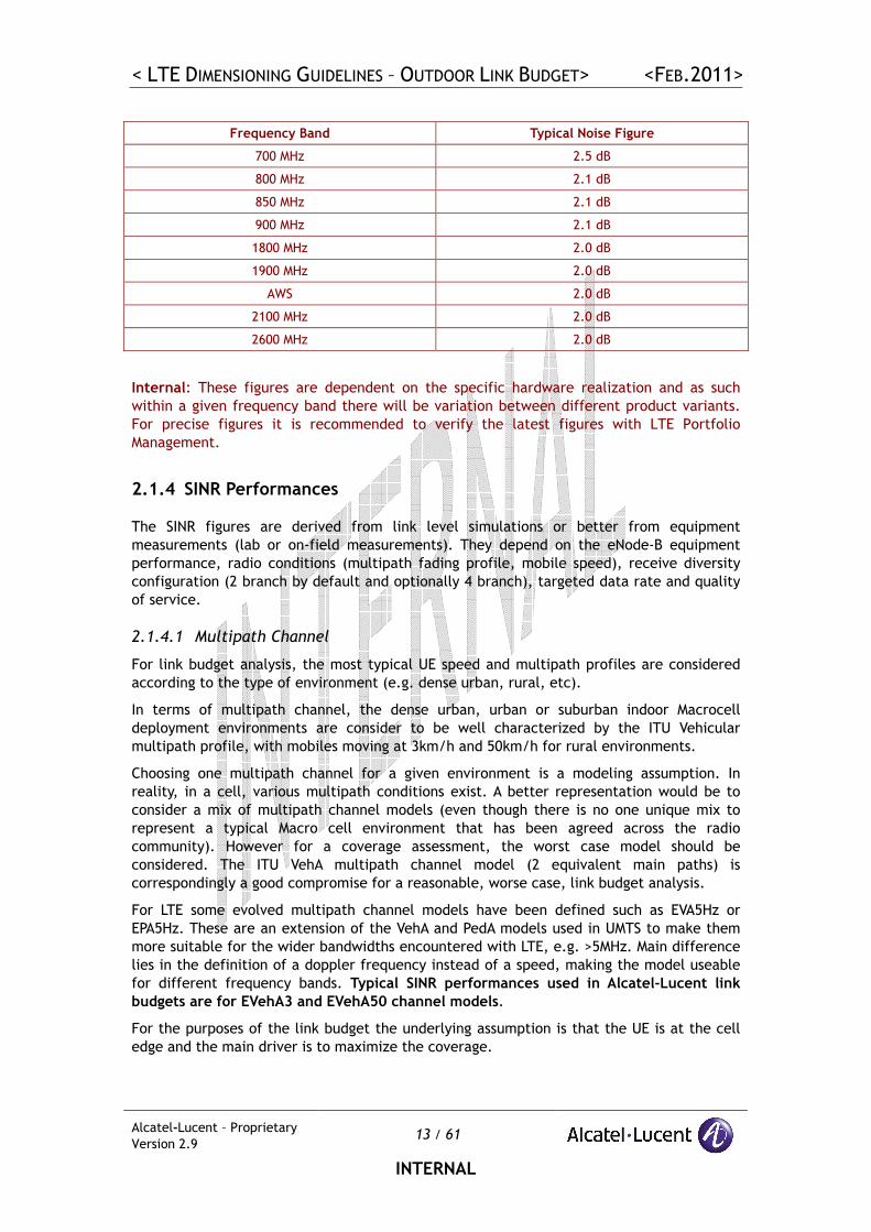
2.1.3 Noise Figure
The Noise Figure of the eNode-B is supplier dependent. Typically the Noise Figures of an
eNode-Bs is 2.5dB.
Internal: Assumed Noise Figures for ALU RRH product variants (September 2010).
< LTE DIMENSIONING GUIDELINES – OUTDOOR LINK BUDGET> <FEB.2011>
Alcatel-Lucent – Proprietary
Version 2.9 13 / 61
INTERNAL
Frequency Band Typical Noise Figure
700 MHz 2.5 dB
800 MHz 2.1 dB
850 MHz 2.1 dB
900 MHz 2.1 dB
1800 MHz 2.0 dB
1900 MHz 2.0 dB
AWS 2.0 dB
2100 MHz 2.0 dB
2600 MHz 2.0 dB
Internal: These figures are dependent on the specific hardware realization and as such
within a given frequency band there will be variation between different product variants.
For precise figures it is recommended to verify the latest figures with LTE Portfolio
Management.
2.1.4 SINR Performances
The SINR figures are derived from link level simulations or better from equipment
measurements (lab or on-field measurements). They depend on the eNode-B equipment
performance, radio conditions (multipath fading profile, mobile speed), receive diversity
configuration (2 branch by default and optionally 4 branch), targeted data rate and quality
of service.
2.1.4.1 Multipath Channel
For link budget analysis, the most typical UE speed and multipath profiles are considered
according to the type of environment (e.g. dense urban, rural, etc).
In terms of multipath channel, the dense urban, urban or suburban indoor Macrocell
deployment environments are consider to be well characterized by the ITU Vehicular
multipath profile, with mobiles moving at 3km/h and 50km/h for rural environments.
Choosing one multipath channel for a given environment is a modeling assumption. In
reality, in a cell, various multipath conditions exist. A better representation would be to
consider a mix of multipath channel models (even though there is no one unique mix to
represent a typical Macro cell environment that has been agreed across the radio
community). However for a coverage assessment, the worst case model should be
considered. The ITU VehA multipath channel model (2 equivalent main paths) is
correspondingly a good compromise for a reasonable, worse case, link budget analysis.
For LTE some evolved multipath channel models have been defined such as EVA5Hz or
EPA5Hz. These are an extension of the VehA and PedA models used in UMTS to make them
more suitable for the wider bandwidths encountered with LTE, e.g. >5MHz. Main difference
lies in the definition of a doppler frequency instead of a speed, making the model useable
for different frequency bands. Typical SINR performances used in Alcatel-Lucent link
budgets are for EVehA3 and EVehA50 channel models.
For the purposes of the link budget the underlying assumption is that the UE is at the cell
edge and the main driver is to maximize the coverage.
< LTE DIMENSIONING GUIDELINES – OUTDOOR LINK BUDGET> <FEB.2011>
Alcatel-Lucent – Proprietary
Version 2.9 14 / 61
INTERNAL
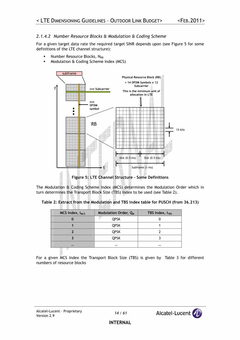
2.1.4.2 Number Resource Blocks & Modulation & Coding Scheme
For a given target data rate the required target SINR depends upon (see Figure 5 for some
definitions of the LTE channel structure):
� Number Resource Blocks, NRB
� Modulation & Coding Scheme Index (MCS)
t
f
one
OFDM symbol
one Subcarrier
Slot (0.5 ms)
Subframe (1 ms)
Slot (0.5 ms)
15 kHz
RB
subframePhysical Resource Block (RB)
= 14 OFDM Symbols x 12 Subcarrier
This is the minimum unit of allocation in LTE
Figure 5: LTE Channel Structure - Some Definitions
The Modulation & Coding Scheme Index (MCS) determines the Modulation Order which in
turn determines the Transport Block Size (TBS) Index to be used (see Table 2).
Table 2: Extract from the Modulation and TBS index table for PUSCH (from 36.213)
MCS Index, IMCS Modulation Order, QM TBS Index, ITBS
0 QPSK 0
1 QPSK 1
2 QPSK 2
3 QPSK 3
… … …
For a given MCS Index the Transport Block Size (TBS) is given by Table 3 for different
numbers of resource blocks
< LTE DIMENSIONING GUIDELINES – OUTDOOR LINK BUDGET> <FEB.2011>
Alcatel-Lucent – Proprietary
Version 2.9 15 / 61
INTERNAL
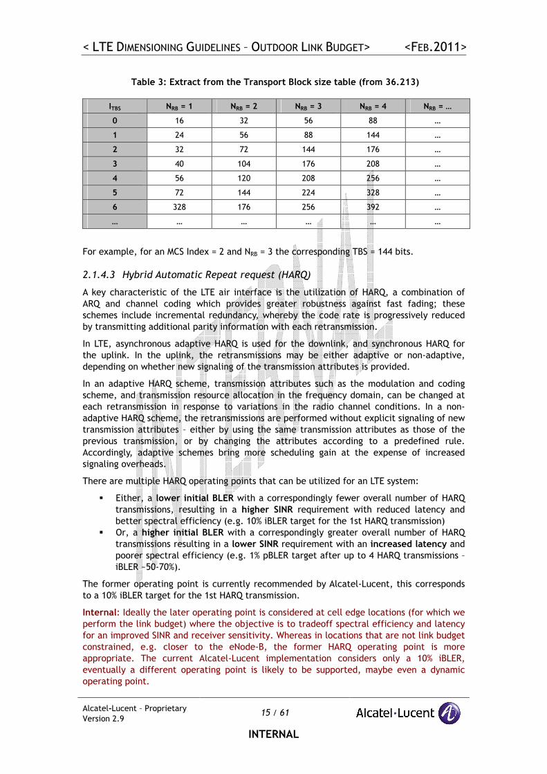
Table 3: Extract from the Transport Block size table (from 36.213)
ITBS NRB = 1 NRB = 2 NRB = 3 NRB = 4 NRB = …
0 16 32 56 88 …
1 24 56 88 144 …
2 32 72 144 176 …
3 40 104 176 208 …
4 56 120 208 256 …
5 72 144 224 328 …
6 328 176 256 392 …
… … … … … …
For example, for an MCS Index = 2 and NRB = 3 the corresponding TBS = 144 bits.
2.1.4.3 Hybrid Automatic Repeat request (HARQ)
A key characteristic of the LTE air interface is the utilization of HARQ, a combination of
ARQ and channel coding which provides greater robustness against fast fading; these
schemes include incremental redundancy, whereby the code rate is progressively reduced
by transmitting additional parity information with each retransmission.
In LTE, asynchronous adaptive HARQ is used for the downlink, and synchronous HARQ for
the uplink. In the uplink, the retransmissions may be either adaptive or non-adaptive,
depending on whether new signaling of the transmission attributes is provided.
In an adaptive HARQ scheme, transmission attributes such as the modulation and coding
scheme, and transmission resource allocation in the frequency domain, can be changed at
each retransmission in response to variations in the radio channel conditions. In a non-
adaptive HARQ scheme, the retransmissions are performed without explicit signaling of new
transmission attributes – either by using the same transmission attributes as those of the
previous transmission, or by changing the attributes according to a predefined rule.
Accordingly, adaptive schemes bring more scheduling gain at the expense of increased
signaling overheads.
There are multiple HARQ operating points that can be utilized for an LTE system:
� Either, a lower initial BLER with a correspondingly fewer overall number of HARQ
transmissions, resulting in a higher SINR requirement with reduced latency and
better spectral efficiency (e.g. 10% iBLER target for the 1st HARQ transmission)
� Or, a higher initial BLER with a correspondingly greater overall number of HARQ
transmissions resulting in a lower SINR requirement with an increased latency and
poorer spectral efficiency (e.g. 1% pBLER target after up to 4 HARQ transmissions –
iBLER ~50-70%).
The former operating point is currently recommended by Alcatel-Lucent, this corresponds
to a 10% iBLER target for the 1st HARQ transmission.
Internal: Ideally the later operating point is considered at cell edge locations (for which we
perform the link budget) where the objective is to tradeoff spectral efficiency and latency
for an improved SINR and receiver sensitivity. Whereas in locations that are not link budget
constrained, e.g. closer to the eNode-B, the former HARQ operating point is more
appropriate. The current Alcatel-Lucent implementation considers only a 10% iBLER,
eventually a different operating point is likely to be supported, maybe even a dynamic
operating point.
< LTE DIMENSIONING GUIDELINES – OUTDOOR LINK BUDGET> <FEB.2011>
Alcatel-Lucent – Proprietary
Version 2.9 16 / 61
INTERNAL
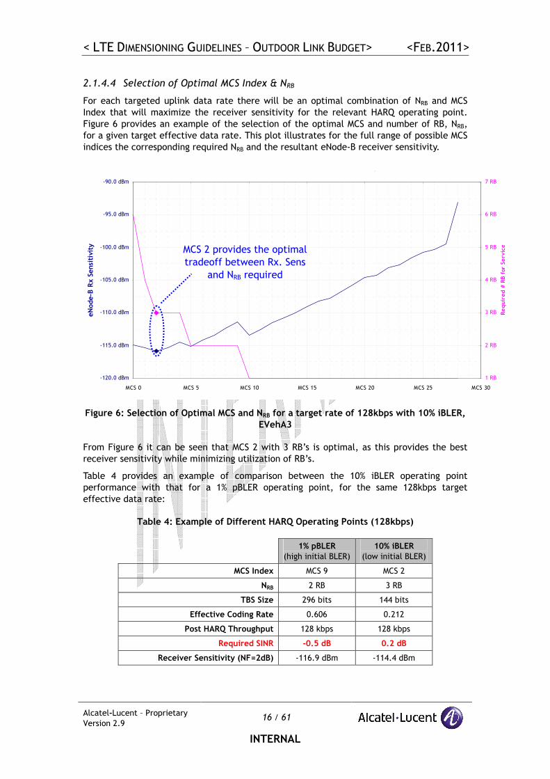
2.1.4.4 Selection of Optimal MCS Index & NRB
For each targeted uplink data rate there will be an optimal combination of NRB and MCS
Index that will maximize the receiver sensitivity for the relevant HARQ operating point.
Figure 6 provides an example of the selection of the optimal MCS and number of RB, NRB,
for a given target effective data rate. This plot illustrates for the full range of possible MCS
indices the corresponding required NRB and the resultant eNode-B receiver sensitivity.
-120.0 dBm
-115.0 dBm
-110.0 dBm
-105.0 dBm
-100.0 dBm
-95.0 dBm
-90.0 dBm
MCS 0 MCS 5 MCS 10 MCS 15 MCS 20 MCS 25 MCS 30
eNode-B Rx Sensitivity
1 RB
2 RB
3 RB
4 RB
5 RB
6 RB
7 RB
Required # RB for Service
Figure 6: Selection of Optimal MCS and NRB for a target rate of 128kbps with 10% iBLER,
EVehA3
From Figure 6 it can be seen that MCS 2 with 3 RB’s is optimal, as this provides the best
receiver sensitivity while minimizing utilization of RB’s.
Table 4 provides an example of comparison between the 10% iBLER operating point
performance with that for a 1% pBLER operating point, for the same 128kbps target
effective data rate:
Table 4: Example of Different HARQ Operating Points (128kbps)
1% pBLER
(high initial BLER)
10% iBLER
(low initial BLER)
MCS Index MCS 9 MCS 2
NRB 2 RB 3 RB
TBS Size 296 bits 144 bits
Effective Coding Rate 0.606 0.212
Post HARQ Throughput 128 kbps 128 kbps
Required SINR -0.5 dB 0.2 dB
Receiver Sensitivity (NF=2dB) -116.9 dBm -114.4 dBm
MCS 2 provides the optimal
tradeoff between Rx. Sens
and NRB required
< LTE DIMENSIONING GUIDELINES – OUTDOOR LINK BUDGET> <FEB.2011>
Alcatel-Lucent – Proprietary
Version 2.9 17 / 61
INTERNAL
Note: The 1% pBLER HARQ operating point (1% BLER after 4 HARQ Tx) corresponds to an
iBLER (BLER for the 1st HARQ transmission) much greater than 10%.
It can be seen from the example summarized in Table 4, that the same required data rate
can be achieved with different combinations of NRB, MCS Index and number of HARQ
transmissions. The receiver sensitivity comparison below highlights the different coverage
for the same targeted data rate due to the different HARQ operating points:
� ( )RBRB(UL)theNode_B10PUSCH_dBdBm .W.N.NF10log SINRySensitivit +=
� Sensitivity1% BLER after 4 HARQ Tx = -0.5 + 10xlog10( 2.0dBxNthx2RBx180kHz ) = -116.9dBm
� Sensitivity10% BLER after 1 HARQ Tx = 0.2 + 10xlog10( 2.0dBxNthx3RBx180kHz ) = -114.4dBm
While the two solutions require a relatively similar SINR, they utilize a different number of
resource blocks, NRB. The trade-off between the two is a combination of the required
bandwidth (number of resource blocks) and the number of HARQ transmissions versus the
receiver sensitivity.
� While the utilization of more HARQ transmissions enhances (reduces) the required
SINR for an equivalent MCS, it also requires the same air interface resources for a
longer period of time (more transmission time intervals).
� Utilizing more resource blocks degrades the receiver sensitivity due to an increased
noise bandwidth (180 kHz x number of resource blocks).
Note that the difference between the receiver sensitivities in Table 4 is due to the
difference in the required SINR and the difference in the number of resource blocks.
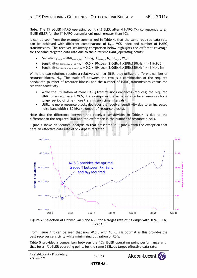
Figure 7 shows an identical analysis to that presented in Figure 6 with the exception that
here an effective data rate of 512kbps is targeted.
-115.0 dBm
-110.0 dBm
-105.0 dBm
-100.0 dBm
-95.0 dBm
-90.0 dBm
MCS 0 MCS 5 MCS 10 MCS 15 MCS 20 MCS 25 MCS 30
eNode-B Rx Sensitivity
1 RB
6 RB
11 RB
16 RB
21 RB
26 RB
Required # RB for Service
Figure 7: Selection of Optimal MCS and NRB for a target rate of 512kbps with 10% iBLER,
EVehA3
From Figure 7 it can be seen that now MCS 3 with 10 RB’s is optimal as this provides the
best receiver sensitivity while minimizing utilization of RB’s.
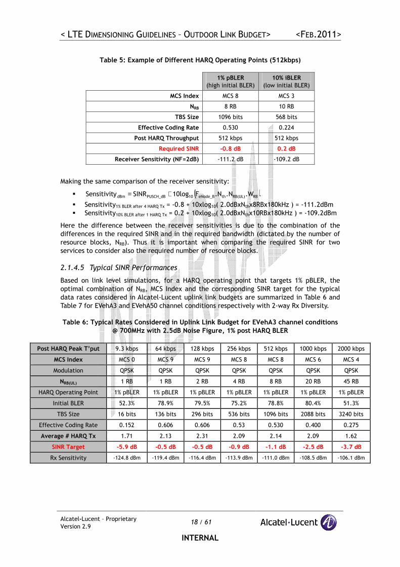
Table 5 provides a comparison between the 10% iBLER operating point performance with
that for a 1% pBLER operating point, for the same 512kbps target effective data rate:
MCS 3 provides the optimal
tradeoff between Rx. Sens
and NRB required
< LTE DIMENSIONING GUIDELINES – OUTDOOR LINK BUDGET> <FEB.2011>
Alcatel-Lucent – Proprietary
Version 2.9 18 / 61
INTERNAL
Table 5: Example of Different HARQ Operating Points (512kbps)
1% pBLER
(high initial BLER)
10% iBLER
(low initial BLER)
MCS Index MCS 8 MCS 3
NRB 8 RB 10 RB
TBS Size 1096 bits 568 bits
Effective Coding Rate 0.530 0.224
Post HARQ Throughput 512 kbps 512 kbps
Required SINR -0.8 dB 0.2 dB
Receiver Sensitivity (NF=2dB) -111.2 dB -109.2 dB
Making the same comparison of the receiver sensitivity:
� ( )RBRB(UL)theNode_B10PUSCH_dBdBm .W.N.NF10log SINRySensitivit +=
� Sensitivity1% BLER after 4 HARQ Tx = -0.8 + 10xlog10( 2.0dBxNthx8RBx180kHz ) = -111.2dBm
� Sensitivity10% BLER after 1 HARQ Tx = 0.2 + 10xlog10( 2.0dBxNthx10RBx180kHz ) = -109.2dBm
Here the difference between the receiver sensitivities is due to the combination of the
differences in the required SINR and in the required bandwidth (dictated by the number of
resource blocks, NRB). Thus it is important when comparing the required SINR for two
services to consider also the required number of resource blocks.
2.1.4.5 Typical SINR Performances
Based on link level simulations, for a HARQ operating point that targets 1% pBLER, the
optimal combination of NRB, MCS Index and the corresponding SINR target for the typical
data rates considered in Alcatel-Lucent uplink link budgets are summarized in Table 6 and
Table 7 for EVehA3 and EVehA50 channel conditions respectively with 2-way Rx Diversity.
Table 6: Typical Rates Considered in Uplink Link Budget for EVehA3 channel conditions
@ 700MHz with 2.5dB Noise Figure, 1% post HARQ BLER
Post HARQ Peak T’put 9.3 kbps 64 kbps 128 kbps 256 kbps 512 kbps 1000 kbps 2000 kbps
MCS Index MCS 0 MCS 9 MCS 9 MCS 8 MCS 8 MCS 6 MCS 4
Modulation QPSK QPSK QPSK QPSK QPSK QPSK QPSK
NRB(UL) 1 RB 1 RB 2 RB 4 RB 8 RB 20 RB 45 RB
HARQ Operating Point 1% pBLER 1% pBLER 1% pBLER 1% pBLER 1% pBLER 1% pBLER 1% pBLER
Initial BLER 52.3% 78.9% 79.5% 75.2% 78.8% 80.4% 51.3%
TBS Size 16 bits 136 bits 296 bits 536 bits 1096 bits 2088 bits 3240 bits
Effective Coding Rate 0.152 0.606 0.606 0.53 0.530 0.400 0.275
Average # HARQ Tx 1.71 2.13 2.31 2.09 2.14 2.09 1.62
SINR Target -5.9 dB -0.5 dB -0.5 dB -0.9 dB -1.1 dB -2.5 dB -3.7 dB
Rx Sensitivity -124.8 dBm -119.4 dBm -116.4 dBm -113.9 dBm -111.0 dBm -108.5 dBm -106.1 dBm
< LTE DIMENSIONING GUIDELINES – OUTDOOR LINK BUDGET> <FEB.2011>
Alcatel-Lucent – Proprietary
Version 2.9 19 / 61
INTERNAL
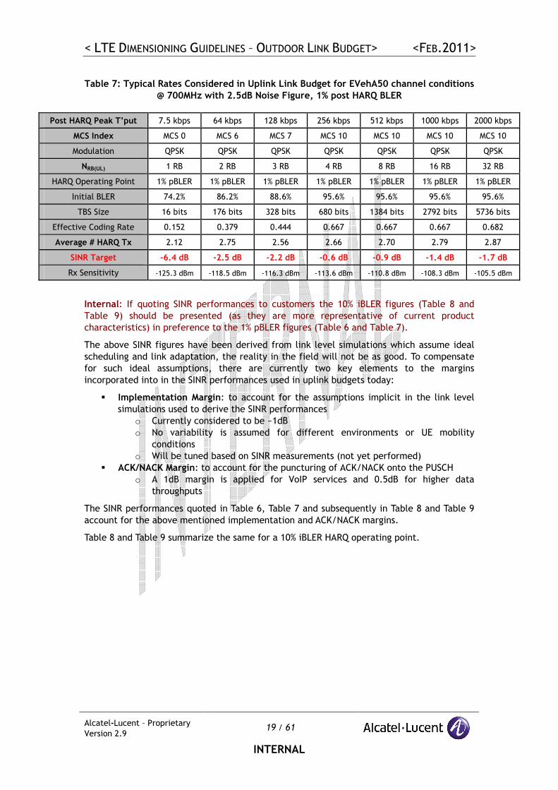
Table 7: Typical Rates Considered in Uplink Link Budget for EVehA50 channel conditions
@ 700MHz with 2.5dB Noise Figure, 1% post HARQ BLER
Post HARQ Peak T’put 7.5 kbps 64 kbps 128 kbps 256 kbps 512 kbps 1000 kbps 2000 kbps
MCS Index MCS 0 MCS 6 MCS 7 MCS 10 MCS 10 MCS 10 MCS 10
Modulation QPSK QPSK QPSK QPSK QPSK QPSK QPSK
NRB(UL) 1 RB 2 RB 3 RB 4 RB 8 RB 16 RB 32 RB
HARQ Operating Point 1% pBLER 1% pBLER 1% pBLER 1% pBLER 1% pBLER 1% pBLER 1% pBLER
Initial BLER 74.2% 86.2% 88.6% 95.6% 95.6% 95.6% 95.6%
TBS Size 16 bits 176 bits 328 bits 680 bits 1384 bits 2792 bits 5736 bits
Effective Coding Rate 0.152 0.379 0.444 0.667 0.667 0.667 0.682
Average # HARQ Tx 2.12 2.75 2.56 2.66 2.70 2.79 2.87
SINR Target -6.4 dB -2.5 dB -2.2 dB -0.6 dB -0.9 dB -1.4 dB -1.7 dB
Rx Sensitivity -125.3 dBm -118.5 dBm -116.3 dBm -113.6 dBm -110.8 dBm -108.3 dBm -105.5 dBm
Internal: If quoting SINR performances to customers the 10% iBLER figures (Table 8 and
Table 9) should be presented (as they are more representative of current product
characteristics) in preference to the 1% pBLER figures (Table 6 and Table 7).
The above SINR figures have been derived from link level simulations which assume ideal
scheduling and link adaptation, the reality in the field will not be as good. To compensate
for such ideal assumptions, there are currently two key elements to the margins
incorporated into in the SINR performances used in uplink budgets today:
� Implementation Margin: to account for the assumptions implicit in the link level
simulations used to derive the SINR performances
o Currently considered to be ~1dB
o No variability is assumed for different environments or UE mobility
conditions
o Will be tuned based on SINR measurements (not yet performed)
� ACK/NACK Margin: to account for the puncturing of ACK/NACK onto the PUSCH
o A 1dB margin is applied for VoIP services and 0.5dB for higher data
throughputs
The SINR performances quoted in Table 6, Table 7 and subsequently in Table 8 and Table 9
account for the above mentioned implementation and ACK/NACK margins.
Table 8 and Table 9 summarize the same for a 10% iBLER HARQ operating point.
< LTE DIMENSIONING GUIDELINES – OUTDOOR LINK BUDGET> <FEB.2011>
Alcatel-Lucent – Proprietary
Version 2.9 20 / 61
INTERNAL
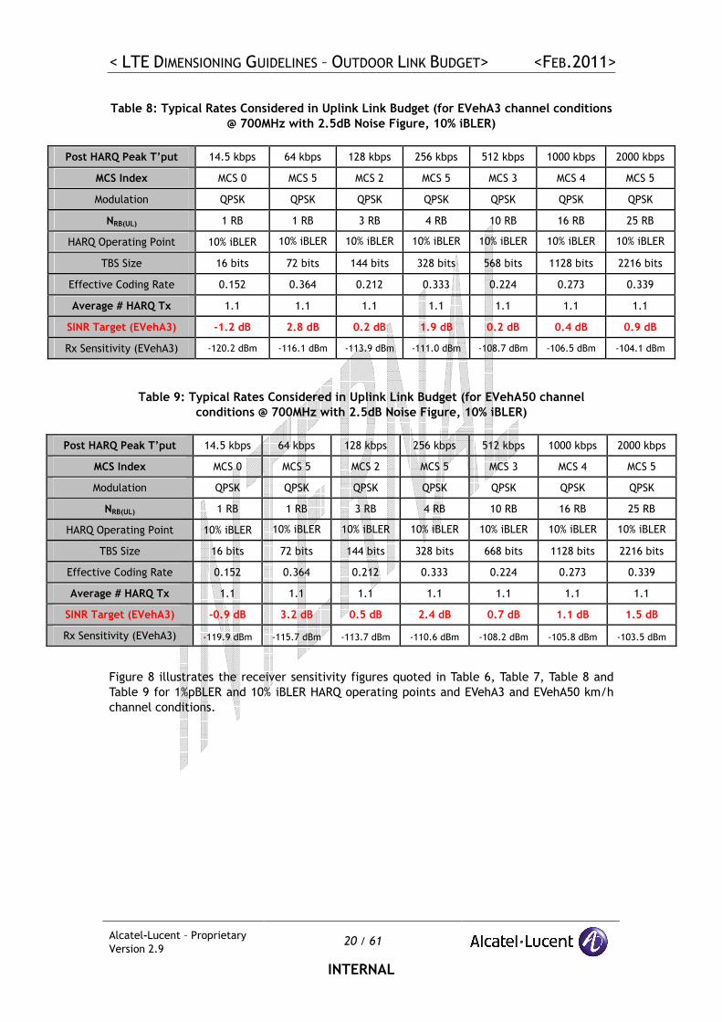
Table 8: Typical Rates Considered in Uplink Link Budget (for EVehA3 channel conditions
@ 700MHz with 2.5dB Noise Figure, 10% iBLER)
Post HARQ Peak T’put 14.5 kbps 64 kbps 128 kbps 256 kbps 512 kbps 1000 kbps 2000 kbps
MCS Index MCS 0 MCS 5 MCS 2 MCS 5 MCS 3 MCS 4 MCS 5
Modulation QPSK QPSK QPSK QPSK QPSK QPSK QPSK
NRB(UL) 1 RB 1 RB 3 RB 4 RB 10 RB 16 RB 25 RB
HARQ Operating Point 10% iBLER 10% iBLER 10% iBLER 10% iBLER 10% iBLER 10% iBLER 10% iBLER
TBS Size 16 bits 72 bits 144 bits 328 bits 568 bits 1128 bits 2216 bits
Effective Coding Rate 0.152 0.364 0.212 0.333 0.224 0.273 0.339
Average # HARQ Tx 1.1 1.1 1.1 1.1 1.1 1.1 1.1
SINR Target (EVehA3) -1.2 dB 2.8 dB 0.2 dB 1.9 dB 0.2 dB 0.4 dB 0.9 dB
Rx Sensitivity (EVehA3) -120.2 dBm -116.1 dBm -113.9 dBm -111.0 dBm -108.7 dBm -106.5 dBm -104.1 dBm
Table 9: Typical Rates Considered in Uplink Link Budget (for EVehA50 channel
conditions @ 700MHz with 2.5dB Noise Figure, 10% iBLER)
Post HARQ Peak T’put 14.5 kbps 64 kbps 128 kbps 256 kbps 512 kbps 1000 kbps 2000 kbps
MCS Index MCS 0 MCS 5 MCS 2 MCS 5 MCS 3 MCS 4 MCS 5
Modulation QPSK QPSK QPSK QPSK QPSK QPSK QPSK
NRB(UL) 1 RB 1 RB 3 RB 4 RB 10 RB 16 RB 25 RB
HARQ Operating Point 10% iBLER 10% iBLER 10% iBLER 10% iBLER 10% iBLER 10% iBLER 10% iBLER
TBS Size 16 bits 72 bits 144 bits 328 bits 668 bits 1128 bits 2216 bits
Effective Coding Rate 0.152 0.364 0.212 0.333 0.224 0.273 0.339
Average # HARQ Tx 1.1 1.1 1.1 1.1 1.1 1.1 1.1
SINR Target (EVehA3) -0.9 dB 3.2 dB 0.5 dB 2.4 dB 0.7 dB 1.1 dB 1.5 dB
Rx Sensitivity (EVehA3) -119.9 dBm -115.7 dBm -113.7 dBm -110.6 dBm -108.2 dBm -105.8 dBm -103.5 dBm
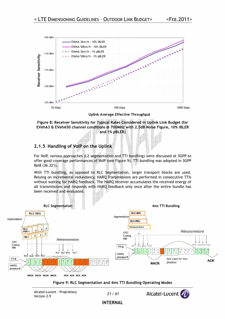
Figure 8 illustrates the receiver sensitivity figures quoted in Table 6, Table 7, Table 8 and
Table 9 for 1%pBLER and 10% iBLER HARQ operating points and EVehA3 and EVehA50 km/h
channel conditions.
< LTE DIMENSIONING GUIDELINES – OUTDOOR LINK BUDGET> <FEB.2011>
Alcatel-Lucent – Proprietary
Version 2.9 21 / 61
INTERNAL
-125 dBm
-120 dBm
-115 dBm
-110 dBm
-105 dBm
10 kbps 100 kbps 1000 kbps
Uplink Average Effective Throughput
Receiver Sensitivity
EVehA 3km/h - 10% iBLER
EVehA 50km/h - 10% iBLER
EVehA 3km/h - 1% pBLER
EVehA 50km/h - 1% pBLER
Figure 8: Receiver Sensitivity for Typical Rates Considered in Uplink Link Budget (for
EVehA3 & EVehA50 channel conditions @ 700MHz with 2.5dB Noise Figure, 10% iBLER
and 1% pBLER)
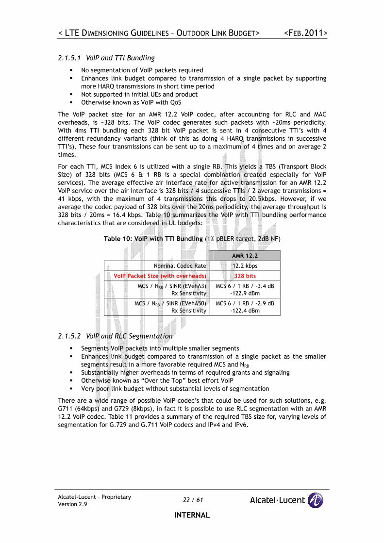
2.1.5 Handling of VoIP on the Uplink
For VoIP, various approaches (L2 segmentation and TTI bundling) were discussed at 3GPP to
offer good coverage performances of VoIP (see Figure 9). TTI bundling was adopted in 3GPP
Rel8 (36.321).
With TTI bundling, as opposed to RLC Segmentation, larger transport blocks are used.
Relying on incremental redundancy, HARQ Transmissions are performed in consecutive TTIs
without waiting for HARQ feedback. The HARQ receiver accumulates the received energy of
all transmissions and responds with HARQ feedback only once after the entire bundle has
been received and evaluated.
RLC Segmentation 4ms TTI Bundling
Figure 9: RLC Segmentation and 4ms TTI Bundling Operating Modes
< LTE DIMENSIONING GUIDELINES – OUTDOOR LINK BUDGET> <FEB.2011>
Alcatel-Lucent – Proprietary
Version 2.9 22 / 61
INTERNAL
2.1.5.1 VoIP and TTI Bundling
� No segmentation of VoIP packets required
� Enhances link budget compared to transmission of a single packet by supporting
more HARQ transmissions in short time period
� Not supported in initial UEs and product
� Otherwise known as VoIP with QoS
The VoIP packet size for an AMR 12.2 VoIP codec, after accounting for RLC and MAC
overheads, is ~328 bits. The VoIP codec generates such packets with ~20ms periodicity.
With 4ms TTI bundling each 328 bit VoIP packet is sent in 4 consecutive TTI’s with 4
different redundancy variants (think of this as doing 4 HARQ transmissions in successive
TTI’s). These four transmissions can be sent up to a maximum of 4 times and on average 2
times.
For each TTI, MCS Index 6 is utilized with a single RB. This yields a TBS (Transport Block
Size) of 328 bits (MCS 6 & 1 RB is a special combination created especially for VoIP
services). The average effective air interface rate for active transmission for an AMR 12.2
VoIP service over the air interface is 328 bits / 4 successive TTIs / 2 average transmissions =
41 kbps, with the maximum of 4 transmissions this drops to 20.5kbps. However, if we
average the codec payload of 328 bits over the 20ms periodicity, the average throughput is
328 bits / 20ms = 16.4 kbps. Table 10 summarizes the VoIP with TTI bundling performance
characteristics that are considered in UL budgets:
Table 10: VoIP with TTI Bundling (1% pBLER target, 2dB NF)
AMR 12.2
Nominal Codec Rate 12.2 kbps
VoIP Packet Size (with overheads) 328 bits
MCS / NRB / SINR (EVehA3)
Rx Sensitivity
MCS 6 / 1 RB / -3.4 dB
-122.9 dBm
MCS / NRB / SINR (EVehA50)
Rx Sensitivity
MCS 6 / 1 RB / -2.9 dB
-122.4 dBm
2.1.5.2 VoIP and RLC Segmentation
� Segments VoIP packets into multiple smaller segments
� Enhances link budget compared to transmission of a single packet as the smaller
segments result in a more favorable required MCS and NRB
� Substantially higher overheads in terms of required grants and signaling
� Otherwise known as “Over the Top” best effort VoIP
� Very poor link budget without substantial levels of segmentation
There are a wide range of possible VoIP codec’s that could be used for such solutions, e.g.
G711 (64kbps) and G729 (8kbps), in fact it is possible to use RLC segmentation with an AMR
12.2 VoIP codec. Table 11 provides a summary of the required TBS size for, varying levels of
segmentation for G.729 and G.711 VoIP codecs and IPv4 and IPv6.
< LTE DIMENSIONING GUIDELINES – OUTDOOR LINK BUDGET> <FEB.2011>
Alcatel-Lucent – Proprietary
Version 2.9 23 / 61
INTERNAL
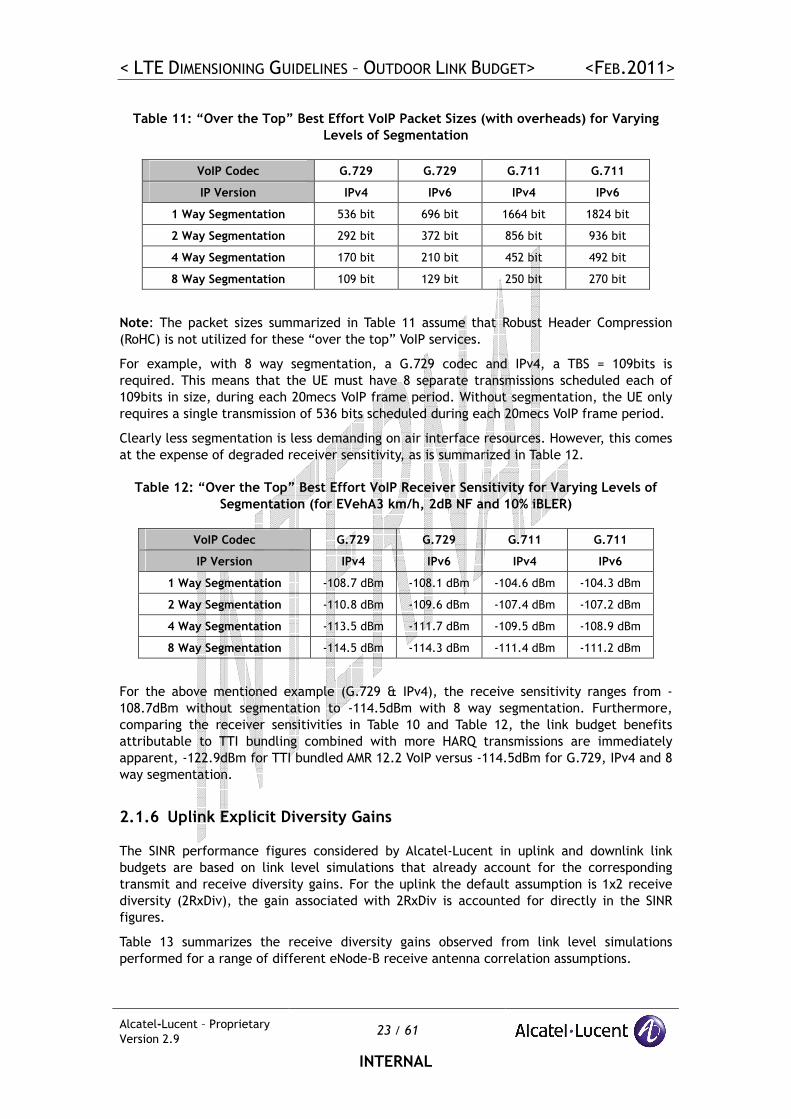
Table 11: “Over the Top” Best Effort VoIP Packet Sizes (with overheads) for Varying
Levels of Segmentation
VoIP Codec G.729 G.729 G.711 G.711
IP Version IPv4 IPv6 IPv4 IPv6
1 Way Segmentation 536 bit 696 bit 1664 bit 1824 bit
2 Way Segmentation 292 bit 372 bit 856 bit 936 bit
4 Way Segmentation 170 bit 210 bit 452 bit 492 bit
8 Way Segmentation 109 bit 129 bit 250 bit 270 bit
Note: The packet sizes summarized in Table 11 assume that Robust Header Compression
(RoHC) is not utilized for these “over the top” VoIP services.
For example, with 8 way segmentation, a G.729 codec and IPv4, a TBS = 109bits is
required. This means that the UE must have 8 separate transmissions scheduled each of
109bits in size, during each 20mecs VoIP frame period. Without segmentation, the UE only
requires a single transmission of 536 bits scheduled during each 20mecs VoIP frame period.
Clearly less segmentation is less demanding on air interface resources. However, this comes
at the expense of degraded receiver sensitivity, as is summarized in Table 12.
Table 12: “Over the Top” Best Effort VoIP Receiver Sensitivity for Varying Levels of
Segmentation (for EVehA3 km/h, 2dB NF and 10% iBLER)
VoIP Codec G.729 G.729 G.711 G.711
IP Version IPv4 IPv6 IPv4 IPv6
1 Way Segmentation -108.7 dBm -108.1 dBm -104.6 dBm -104.3 dBm
2 Way Segmentation -110.8 dBm -109.6 dBm -107.4 dBm -107.2 dBm
4 Way Segmentation -113.5 dBm -111.7 dBm -109.5 dBm -108.9 dBm
8 Way Segmentation -114.5 dBm -114.3 dBm -111.4 dBm -111.2 dBm
For the above mentioned example (G.729 & IPv4), the receive sensitivity ranges from -
108.7dBm without segmentation to -114.5dBm with 8 way segmentation. Furthermore,
comparing the receiver sensitivities in Table 10 and Table 12, the link budget benefits
attributable to TTI bundling combined with more HARQ transmissions are immediately
apparent, -122.9dBm for TTI bundled AMR 12.2 VoIP versus -114.5dBm for G.729, IPv4 and 8
way segmentation.
2.1.6 Uplink Explicit Diversity Gains
The SINR performance figures considered by Alcatel-Lucent in uplink and downlink link
budgets are based on link level simulations that already account for the corresponding
transmit and receive diversity gains. For the uplink the default assumption is 1x2 receive
diversity (2RxDiv), the gain associated with 2RxDiv is accounted for directly in the SINR
figures.
Table 13 summarizes the receive diversity gains observed from link level simulations
performed for a range of different eNode-B receive antenna correlation assumptions.
< LTE DIMENSIONING GUIDELINES – OUTDOOR LINK BUDGET> <FEB.2011>
Alcatel-Lucent – Proprietary
Version 2.9 24 / 61
INTERNAL
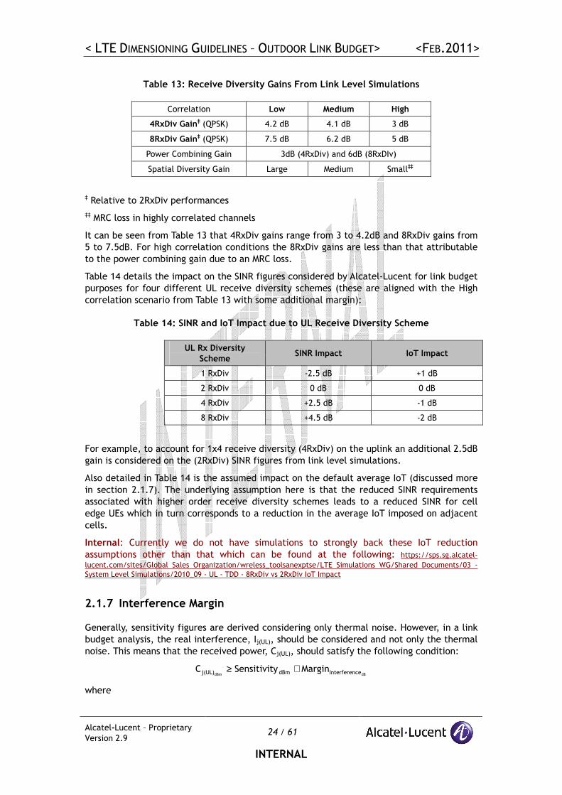
Table 13: Receive Diversity Gains From Link Level Simulations
Correlation Low Medium High
4RxDiv Gain‡ (QPSK) 4.2 dB 4.1 dB 3 dB
8RxDiv Gain‡ (QPSK) 7.5 dB 6.2 dB 5 dB
Power Combining Gain 3dB (4RxDiv) and 6dB (8RxDIv)
Spatial Diversity Gain Large Medium Small‡‡
‡ Relative to 2RxDiv performances
‡‡ MRC loss in highly correlated channels
It can be seen from Table 13 that 4RxDiv gains range from 3 to 4.2dB and 8RxDiv gains from
5 to 7.5dB. For high correlation conditions the 8RxDiv gains are less than that attributable
to the power combining gain due to an MRC loss.
Table 14 details the impact on the SINR figures considered by Alcatel-Lucent for link budget
purposes for four different UL receive diversity schemes (these are aligned with the High
correlation scenario from Table 13 with some additional margin):
Table 14: SINR and IoT Impact due to UL Receive Diversity Scheme
UL Rx Diversity
Scheme SINR Impact IoT Impact
1 RxDiv -2.5 dB +1 dB
2 RxDiv 0 dB 0 dB
4 RxDiv +2.5 dB -1 dB
8 RxDiv +4.5 dB -2 dB
For example, to account for 1x4 receive diversity (4RxDiv) on the uplink an additional 2.5dB
gain is considered on the (2RxDiv) SINR figures from link level simulations.
Also detailed in Table 14 is the assumed impact on the default average IoT (discussed more
in section 2.1.7). The underlying assumption here is that the reduced SINR requirements
associated with higher order receive diversity schemes leads to a reduced SINR for cell
edge UEs which in turn corresponds to a reduction in the average IoT imposed on adjacent
cells.
Internal: Currently we do not have simulations to strongly back these IoT reduction
assumptions other than that which can be found at the following: https://sps.sg.alcatel-
lucent.com/sites/Global Sales Organization/wreless_toolsanexptse/LTE Simulations WG/Shared Documents/03 -
System Level Simulations/2010_09 - UL - TDD - 8RxDiv vs 2RxDiv IoT Impact
2.1.7 Interference Margin
Generally, sensitivity figures are derived considering only thermal noise. However, in a link
budget analysis, the real interference, Ij(UL), should be considered and not only the thermal
noise. This means that the received power, Cj(UL), should satisfy the following condition:
dBdBm ceInterferendBmj(UL) MarginySensitivitC +≥
where
< LTE DIMENSIONING GUIDELINES – OUTDOOR LINK BUDGET> <FEB.2011>
Alcatel-Lucent – Proprietary
Version 2.9 25 / 61
INTERNAL
+=
WN
WNI10logMargin
th
thj(UL)
ceInterferen dB
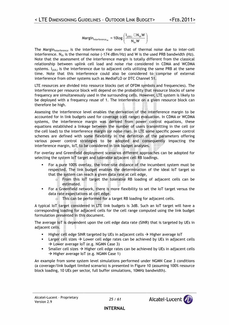
The MarginInterference is the interference rise over that of thermal noise due to inter-cell
interference. Nth is the thermal noise (-174 dBm/Hz) and W is the used PRB bandwidth (Hz).
Note that the assessment of the interference margin is totally different from the classical
relationship between uplink cell load and noise rise considered in CDMA and WCDMA
systems. Ij(UL) is the interference due to adjacent cells utilizing the same PRB at the same
time. Note that this interference could also be considered to comprise of external
interference from other systems such as MediaFLO or DTC Channel 51.
LTE resources are divided into resource blocks (set of OFDM symbols and frequencies). The
interference per resource block will depend on the probability that resource blocks of same
frequency are simultaneously used in the surrounding cells. However, LTE system is likely to
be deployed with a frequency reuse of 1. The interference on a given resource block can
therefore be high.
Assessing the interference level enables the derivation of the interference margin to be
accounted for in link budgets used for coverage (cell range) evaluation. In CDMA or WCDMA
systems, the interference margin was derived from power control equations, these
equations established a linkage between the number of users transmitting in the cell (or
the cell load) to the interference margin (or noise rise). In LTE some specific power control
schemes are defined with some flexibility in the definition of the parameters offering
various power control strategies to be adopted and consequently impacting the
interference margin, IoT, to be considered in link budget analyses.
For overlay and Greenfield deployment scenarios different approaches can be adopted for
selecting the system IoT target and tolerable adjacent cell RB loadings.
� For a pure 100% overlay, the inter-site distance of the incumbent system must be
respected. The link budget enables the determination of the ideal IoT target so
that the system can reach a given data rate at cell edge,
o From this IoT target the tolerable RB loading of adjacent cells can be
estimated.
� For a Greenfield network, there is more flexibility to set the IoT target versus the
data rate expectations at cell edge.
o This can be performed for a target RB loading for adjacent cells.
A typical IoT target considered in LTE link budgets is 3dB. Such an IoT target will have a
corresponding loading for adjacent cells for the cell range computed using the link budget
formulation presented in this document.
The average IoT is dependent upon the cell edge data rate (SINR) that is targeted by UEs in
adjacent cells.
� Higher cell edge SINR targeted by UEs in adjacent cells � Higher average IoT
� Larger cell sizes � Lower cell edge rates can be achieved by UEs in adjacent cells
� Lower average IoT (e.g. NGMN Case 3)
� Smaller cell sizes � Higher cell edge rates can be achieved by UEs in adjacent cells
� Higher average IoT (e.g. NGMN Case 1)
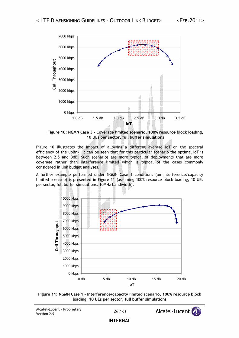
An example from some system level simulations performed under NGMN Case 3 conditions
(a coverage/link budget limited scenario) is presented in Figure 10 (assuming 100% resource
block loading, 10 UEs per sector, full buffer simulations, 10MHz bandwidth).
< LTE DIMENSIONING GUIDELINES – OUTDOOR LINK BUDGET> <FEB.2011>
Alcatel-Lucent – Proprietary
Version 2.9 26 / 61
INTERNAL
0 kbps
1000 kbps
2000 kbps
3000 kbps
4000 kbps
5000 kbps
6000 kbps
7000 kbps
1.0 dB 1.5 dB 2.0 dB 2.5 dB 3.0 dB 3.5 dB
IoT
Cell Throughput
Figure 10: NGMN Case 3 – Coverage limited scenario, 100% resource block loading,
10 UEs per sector, full buffer simulations
Figure 10 illustrates the impact of allowing a different average IoT on the spectral
efficiency of the uplink. It can be seen that for this particular scenario the optimal IoT is
between 2.5 and 3dB. Such scenarios are more typical of deployments that are more
coverage rather than interference limited which is typical of the cases commonly
considered in link budget analyses.
A further example performed under NGMN Case 1 conditions (an interference/capacity
limited scenario) is presented in Figure 11 (assuming 100% resource block loading, 10 UEs
per sector, full buffer simulations, 10MHz bandwidth).
0 kbps
1000 kbps
2000 kbps
3000 kbps
4000 kbps
5000 kbps
6000 kbps
7000 kbps
8000 kbps
9000 kbps
10000 kbps
0 dB 5 dB 10 dB 15 dB 20 dB
IoT
Cell Throughput
Figure 11: NGMN Case 1 – Interference/capacity limited scenario, 100% resource block
loading, 10 UEs per sector, full buffer simulations
< LTE DIMENSIONING GUIDELINES – OUTDOOR LINK BUDGET> <FEB.2011>
Alcatel-Lucent – Proprietary
Version 2.9 27 / 61
INTERNAL
Figure 11 illustrates the impact of allowing a different average IoT on the spectral
efficiency of the uplink. It can be seen that for this particular scenario the optimal IoT is
greater than 5dB. However, in this case the link budget is not constraining and thus from a
link budget perspective there is no issue with tolerating a higher IoT.
Note that while the simulations indicate there are gains to be had at IoTs of up to 15dB or
more, operating points greater ~5.5dB are not currently recommended by Alcatel-Lucent.
As was mentioned in section 2.1.6, when considering different receive diversity schemes,
the default IoT recommendations are offset according to the figures recommended in Table
14.
2.1.8 Shadowing Margin
From the previous section, the link budget should satisfy the following equation:
dBdBm ceInterferendBmj(UL) MarginySensitivitC +≥
This equation should be satisfied from a statistical point of view with a given probability,
Pcov, (coverage probability) within the cell. Typically, the received power should be better
than the sensitivity over more than 95% of the cell area:
( ) covceInterferendBmj(UL) PMarginySensitivitCProbadBdBm
≥+≥
Generally, a target of 95% cell coverage is considered in dense urban, urban and suburban
environments, while 90% is considered in rural environments, but this is dictated by the
operator’s coverage quality objectives.
The received power from a mobile within the cell will depend upon the shadowing
conditions due to obstacles between the UE and the base station antennas. These slow
shadowing variations (in dB) can be represented as a Gaussian random variable with a zero-
mean and a standard deviation that is dependent upon the environment (typically between
5 to 10 dB).
Due to the Gaussian properties of the shadowing, a margin called the “shadowing margin”
can be computed and incorporated in the link budget calculations to consider the coverage
probability requirement, either probability at cell edge or over the cell. The following
formulas are used to derive the shadowing margins according to the specified coverage
probability:
−=
2σ
Marginerfc
2
11P dBShadowing
border cell cov
( )
+−++=+
b
ab1erf1eaerf1
2
1 P
2b
2ab1
area cell cov
Where
� 2σ
Margina
Shadowing=
� ( ) 2σ10ln
K b 2=
� K2 is the propagation model coefficient.
More details on the way these equations are derived can be found in [1].
< LTE DIMENSIONING GUIDELINES – OUTDOOR LINK BUDGET> <FEB.2011>
Alcatel-Lucent – Proprietary
Version 2.9 28 / 61
INTERNAL
In order to guarantee a given level of indoor coverage, a penetration margin is considered
in the link budget (see sections 2.1 and 2.1.11). Either this penetration margin is defined as
a worst-case (e.g. 95th percentile value) value for which indoor coverage must be ensured
or as an average penetration loss value with an associated standard deviation. In the
former case, both variations of penetration and shadowing can be considered together
through a single Gaussian random variable with the following composite standard deviation:
2npenetratio
2shadowing σσσ +=
In order to simplify the link budget it is recommended to consider the former approach, i.e.
the penetration margin defined in Section 2.1.11 is therefore considered as a worst case
value, without the requirement to consider any additional standard deviation.
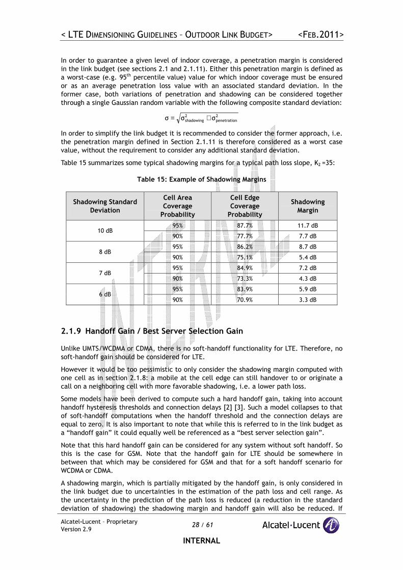
Table 15 summarizes some typical shadowing margins for a typical path loss slope, K2 =35:
Table 15: Example of Shadowing Margins
Shadowing Standard
Deviation
Cell Area
Coverage
Probability
Cell Edge
Coverage
Probability
Shadowing
Margin
95% 87.7% 11.7 dB 10 dB
90% 77.7% 7.7 dB
95% 86.2% 8.7 dB 8 dB
90% 75.1% 5.4 dB
95% 84.9% 7.2 dB 7 dB
90% 73.3% 4.3 dB
95% 83.9% 5.9 dB 6 dB
90% 70.9% 3.3 dB
2.1.9 Handoff Gain / Best Server Selection Gain
Unlike UMTS/WCDMA or CDMA, there is no soft-handoff functionality for LTE. Therefore, no
soft-handoff gain should be considered for LTE.
However it would be too pessimistic to only consider the shadowing margin computed with
one cell as in section 2.1.8: a mobile at the cell edge can still handover to or originate a
call on a neighboring cell with more favorable shadowing, i.e. a lower path loss.
Some models have been derived to compute such a hard handoff gain, taking into account
handoff hysteresis thresholds and connection delays [2] [3]. Such a model collapses to that
of soft-handoff computations when the handoff threshold and the connection delays are
equal to zero. It is also important to note that while this is referred to in the link budget as
a “handoff gain” it could equally well be referenced as a “best server selection gain”.
Note that this hard handoff gain can be considered for any system without soft handoff. So
this is the case for GSM. Note that the handoff gain for LTE should be somewhere in
between that which may be considered for GSM and that for a soft handoff scenario for
WCDMA or CDMA.
A shadowing margin, which is partially mitigated by the handoff gain, is only considered in
the link budget due to uncertainties in the estimation of the path loss and cell range. As
the uncertainty in the prediction of the path loss is reduced (a reduction in the standard
deviation of shadowing) the shadowing margin and handoff gain will also be reduced. If
< LTE DIMENSIONING GUIDELINES – OUTDOOR LINK BUDGET> <FEB.2011>
Alcatel-Lucent – Proprietary
Version 2.9 29 / 61
INTERNAL
there are no uncertainties in the estimation of the path loss and the corresponding cell
range, there will be no need to consider any shadowing margin or handoff gain.
Internal: However we are not used to considering such a gain in GSM. It is highly
recommended to consider such a hard handoff gain, above all to have favorable link budget
comparison with CDMA or WCDMA, both of which consider a soft handoff gain in their link
budgets.
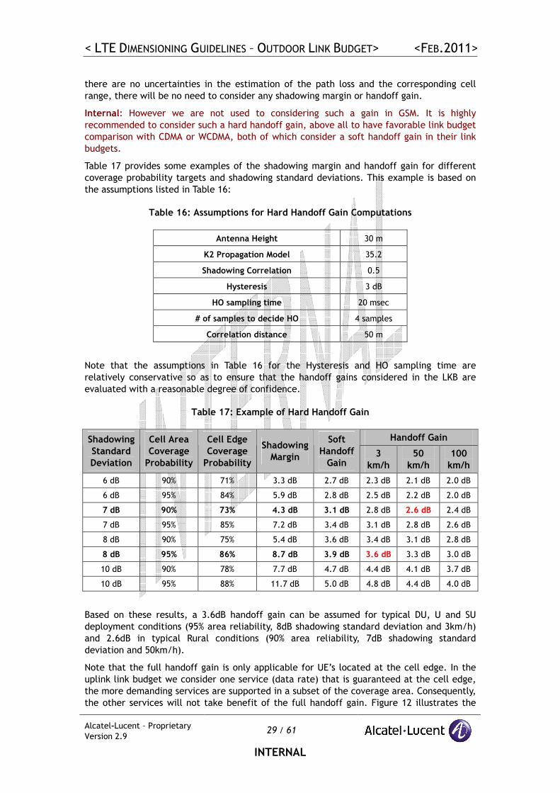
Table 17 provides some examples of the shadowing margin and handoff gain for different
coverage probability targets and shadowing standard deviations. This example is based on
the assumptions listed in Table 16:
Table 16: Assumptions for Hard Handoff Gain Computations
Antenna Height 30 m
K2 Propagation Model 35.2
Shadowing Correlation 0.5
Hysteresis 3 dB
HO sampling time 20 msec
# of samples to decide HO 4 samples
Correlation distance 50 m
Note that the assumptions in Table 16 for the Hysteresis and HO sampling time are
relatively conservative so as to ensure that the handoff gains considered in the LKB are
evaluated with a reasonable degree of confidence.
Table 17: Example of Hard Handoff Gain
Handoff Gain Shadowing
Standard
Deviation
Cell Area
Coverage
Probability
Cell Edge
Coverage
Probability
Shadowing
Margin
Soft
Handoff
Gain 3
km/h
50
km/h
100
km/h
6 dB 90% 71% 3.3 dB 2.7 dB 2.3 dB 2.1 dB 2.0 dB
6 dB 95% 84% 5.9 dB 2.8 dB 2.5 dB 2.2 dB 2.0 dB
7 dB 90% 73% 4.3 dB 3.1 dB 2.8 dB 2.6 dB 2.4 dB
7 dB 95% 85% 7.2 dB 3.4 dB 3.1 dB 2.8 dB 2.6 dB
8 dB 90% 75% 5.4 dB 3.6 dB 3.4 dB 3.1 dB 2.8 dB
8 dB 95% 86% 8.7 dB 3.9 dB 3.6 dB 3.3 dB 3.0 dB
10 dB 90% 78% 7.7 dB 4.7 dB 4.4 dB 4.1 dB 3.7 dB
10 dB 95% 88% 11.7 dB 5.0 dB 4.8 dB 4.4 dB 4.0 dB
Based on these results, a 3.6dB handoff gain can be assumed for typical DU, U and SU
deployment conditions (95% area reliability, 8dB shadowing standard deviation and 3km/h)
and 2.6dB in typical Rural conditions (90% area reliability, 7dB shadowing standard
deviation and 50km/h).
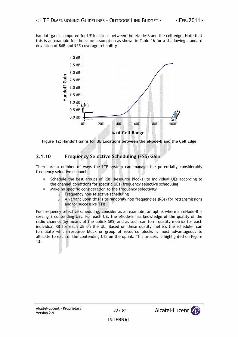
Note that the full handoff gain is only applicable for UE’s located at the cell edge. In the
uplink link budget we consider one service (data rate) that is guaranteed at the cell edge,
the more demanding services are supported in a subset of the coverage area. Consequently,
the other services will not take benefit of the full handoff gain. Figure 12 illustrates the
< LTE DIMENSIONING GUIDELINES – OUTDOOR LINK BUDGET> <FEB.2011>
Alcatel-Lucent – Proprietary
Version 2.9 30 / 61
INTERNAL
handoff gains computed for UE locations between the eNode-B and the cell edge. Note that
this is an example for the same assumption as shown in Table 16 for a shadowing standard
deviation of 8dB and 95% coverage reliability.
0.0 dB
0.5 dB
1.0 dB
1.5 dB
2.0 dB
2.5 dB
3.0 dB
3.5 dB
4.0 dB
0% 20% 40% 60% 80% 100%
% of Cell Range
Handoff Gain
Figure 12: Handoff Gains for UE Locations between the eNode-B and the Cell Edge
2.1.10 Frequency Selective Scheduling (FSS) Gain
There are a number of ways the LTE system can manage the potentially considerably
frequency selective channel:
� Schedule the best groups of RBs (Resource Blocks) to individual UEs according to
the channel conditions for specific UEs (frequency selective scheduling)
� Make no specific consideration to the frequency selectivity
o Frequency non-selective scheduling
o A variant upon this is to randomly hop frequencies (RBs) for retransmissions
and/or successive TTIs
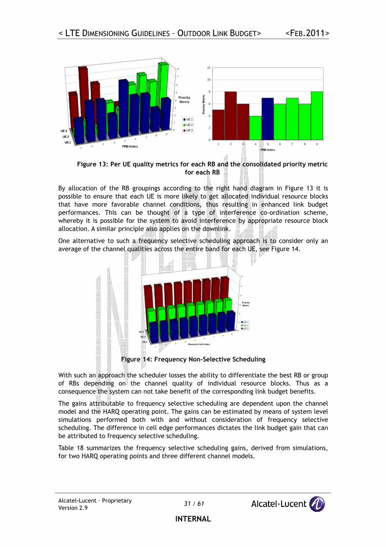
For frequency selective scheduling, consider as an example, an uplink where an eNode-B is
serving 3 contending UEs. For each UE, the eNode-B has knowledge of the quality of the
radio channel (by means of the uplink SRS) and as such can form quality metrics for each
individual RB for each UE on the UL. Based on these quality metrics the scheduler can
formulate which resource block or group of resource blocks is most advantageous to
allocate to each of the contending UEs on the uplink. This process is highlighted on Figure
13.
< LTE DIMENSIONING GUIDELINES – OUTDOOR LINK BUDGET> <FEB.2011>
Alcatel-Lucent – Proprietary
Version 2.9 31 / 61
INTERNAL
12
34
56
78
9
UE 1
UE 2
UE 3 0
1
2
3
4
5
6
7
8
Priority Metric
PRB Index
UE 1
UE 2
UE 3
0
2
4
6
8
10
12
1 2 3 4 5 6 7 8 9
PRB Index
Prio
rity
Met
ric
Figure 13: Per UE quality metrics for each RB and the consolidated priority metric
for each RB
By allocation of the RB groupings according to the right hand diagram in Figure 13 it is
possible to ensure that each UE is more likely to get allocated individual resource blocks
that have more favorable channel conditions, thus resulting in enhanced link budget
performances. This can be thought of a type of interference co-ordination scheme,
whereby it is possible for the system to avoid interference by appropriate resource block
allocation. A similar principle also applies on the downlink.
One alternative to such a frequency selective scheduling approach is to consider only an
average of the channel qualities across the entire band for each UE, see Figure 14.
12
34
56
78
9
UE 1
UE 2
UE 30
1
2
3
4
5
6
Priority Metric
Resource Unit Index
UE 1UE 2UE 3
Figure 14: Frequency Non-Selective Scheduling
With such an approach the scheduler losses the ability to differentiate the best RB or group
of RBs depending on the channel quality of individual resource blocks. Thus as a
consequence the system can not take benefit of the corresponding link budget benefits.
The gains attributable to frequency selective scheduling are dependent upon the channel
model and the HARQ operating point. The gains can be estimated by means of system level
simulations performed both with and without consideration of frequency selective
scheduling. The difference in cell edge performances dictates the link budget gain that can
be attributed to frequency selective scheduling.
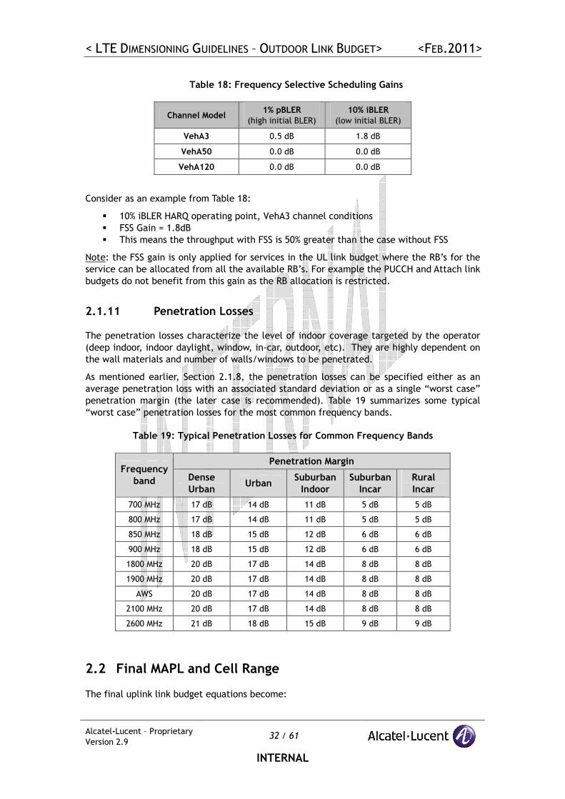
Table 18 summarizes the frequency selective scheduling gains, derived from simulations,
for two HARQ operating points and three different channel models.
< LTE DIMENSIONING GUIDELINES – OUTDOOR LINK BUDGET> <FEB.2011>
Alcatel-Lucent – Proprietary
Version 2.9 32 / 61
INTERNAL
Table 18: Frequency Selective Scheduling Gains
Channel Model 1% pBLER
(high initial BLER)
10% iBLER
(low initial BLER)
VehA3 0.5 dB 1.8 dB
VehA50 0.0 dB 0.0 dB
VehA120 0.0 dB 0.0 dB
Consider as an example from Table 18:
� 10% iBLER HARQ operating point, VehA3 channel conditions
� FSS Gain = 1.8dB
� This means the throughput with FSS is 50% greater than the case without FSS
Note: the FSS gain is only applied for services in the UL link budget where the RB’s for the
service can be allocated from all the available RB’s. For example the PUCCH and Attach link
budgets do not benefit from this gain as the RB allocation is restricted.
2.1.11 Penetration Losses
The penetration losses characterize the level of indoor coverage targeted by the operator
(deep indoor, indoor daylight, window, in-car, outdoor, etc). They are highly dependent on
the wall materials and number of walls/windows to be penetrated.
As mentioned earlier, Section 2.1.8, the penetration losses can be specified either as an
average penetration loss with an associated standard deviation or as a single “worst case”
penetration margin (the later case is recommended). Table 19 summarizes some typical
“worst case” penetration losses for the most common frequency bands.
Table 19: Typical Penetration Losses for Common Frequency Bands
Penetration Margin Frequency
band Dense
Urban Urban
Suburban
Indoor
Suburban
Incar
Rural
Incar
700 MHz 17 dB 14 dB 11 dB 5 dB 5 dB
800 MHz 17 dB 14 dB 11 dB 5 dB 5 dB
850 MHz 18 dB 15 dB 12 dB 6 dB 6 dB
900 MHz 18 dB 15 dB 12 dB 6 dB 6 dB
1800 MHz 20 dB 17 dB 14 dB 8 dB 8 dB
1900 MHz 20 dB 17 dB 14 dB 8 dB 8 dB
AWS 20 dB 17 dB 14 dB 8 dB 8 dB
2100 MHz 20 dB 17 dB 14 dB 8 dB 8 dB
2600 MHz 21 dB 18 dB 15 dB 9 dB 9 dB
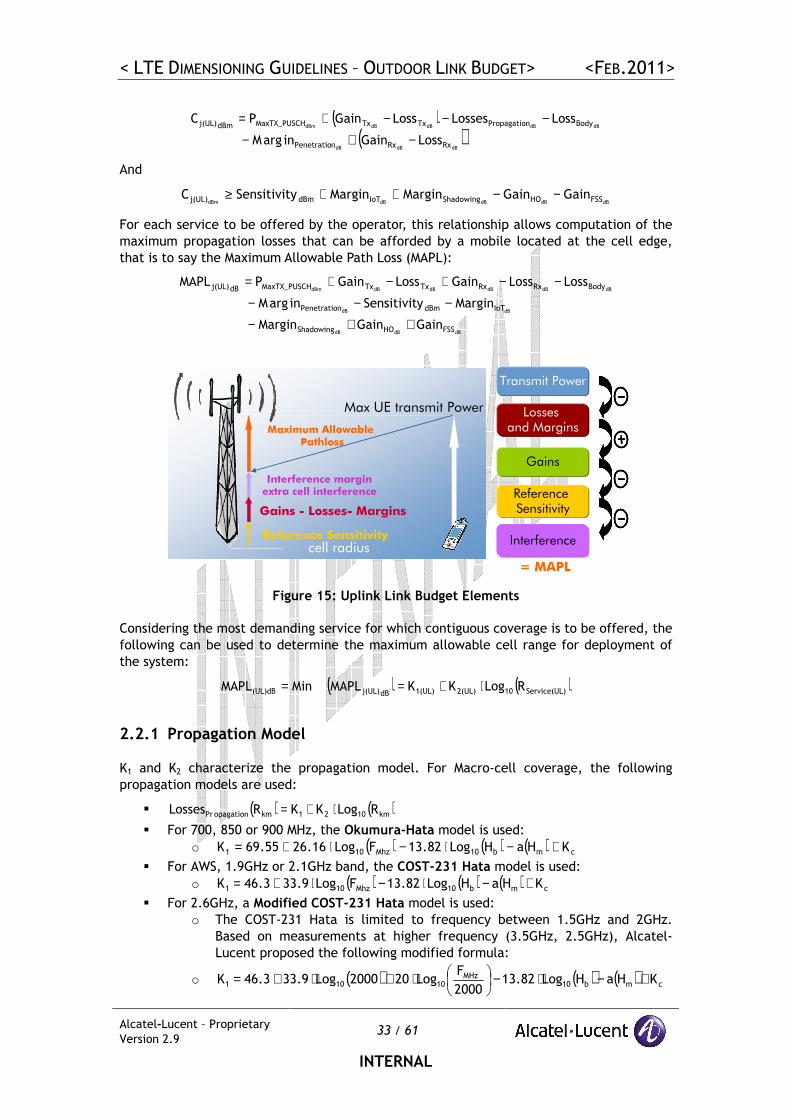
2.2 Final MAPL and Cell Range
The final uplink link budget equations become:
< LTE DIMENSIONING GUIDELINES – OUTDOOR LINK BUDGET> <FEB.2011>
Alcatel-Lucent – Proprietary
Version 2.9 33 / 61
INTERNAL
( )( )
dBdBdB
dBdBdBdBdBm
RxRxnPenetratio
BodynPropagatioTxTxHMaxTX_PUSCdBmj(UL)
LossGaininargM
ssLoLossesLossGainPC
−+−
−−−+=
And
dBdBdBdBdBm FSSHOShadowingIoTdBmj(UL) GainGainMarginMarginySensitivitC −−++≥
For each service to be offered by the operator, this relationship allows computation of the
maximum propagation losses that can be afforded by a mobile located at the cell edge,
that is to say the Maximum Allowable Path Loss (MAPL):
dBdBdB
dBdB
dBdBdBdBdBdBm
FSSHOShadowing
IoTdBmnPenetratio
BodyRxRxTxTxHMaxTX_PUSCdBj(UL)
GainGainMargin
MarginySensitivitinargM
LossossLGainossLGainPMAPL
++−
−−−
−−+−+=
Reference Sensitivity
Transmit Power
Losses and Margins
Gains
•= MAPL
Interferencecell radius
Maximum Allowable Pathloss
Reference Sensitivity
Max UE transmit Power
Gains - Losses- Margins
Interference marginextra cell interference
Figure 15: Uplink Link Budget Elements
Considering the most demanding service for which contiguous coverage is to be offered, the
following can be used to determine the maximum allowable cell range for deployment of
the system:
( ) ( ))Service(UL102(UL)1(UL)dBj(UL)(UL)dB RLogKKMAPLMinMAPL ⋅+==
2.2.1 Propagation Model
K1 and K2 characterize the propagation model. For Macro-cell coverage, the following
propagation models are used:
� ( ) ( )km1021kmopagationPr RLogKKRossesL ⋅+=
� For 700, 850 or 900 MHz, the Okumura-Hata model is used:
o ( ) ( ) ( ) cmb10Mhz101 KHaHLog82.13FLog16.2655.69K +−⋅−⋅+=
� For AWS, 1.9GHz or 2.1GHz band, the COST-231 Hata model is used:
o ( ) ( ) ( ) cmb10Mhz101 KHaHLog82.13FLog9.333.46K +−⋅−⋅+=
� For 2.6GHz, a Modified COST-231 Hata model is used:
o The COST-231 Hata is limited to frequency between 1.5GHz and 2GHz.
Based on measurements at higher frequency (3.5GHz, 2.5GHz), Alcatel-
Lucent proposed the following modified formula:
o ( ) ( ) ( ) cmb10MHz
10101 KHaHLog82.132000
FLog202000Log9.333.46K +−⋅−
⋅+⋅+=
< LTE DIMENSIONING GUIDELINES – OUTDOOR LINK BUDGET> <FEB.2011>
Alcatel-Lucent – Proprietary
Version 2.9 34 / 61
INTERNAL
o The Modified Cost-231 Hata model is only considered applicable for
Suburban and Rural morphologies. For Dense Urban and Urban morphologies
the Cost-231 Hata model is considered to be a better representation.
� Where
o ( )b102 HLog55.69.44K ⋅−=
o ( ) [ ] 597.4) xH(11.75(Log3.2 2m10 −>−⋅= cm KforHa
o ( ) ( )[ ] [ ] 50.8-)(FLog1.567.01.1 MHz1010 −≤⋅−⋅−⋅= cmMHzm KforHFLogHa
FMHz represents the operating frequency in MHz. Hb is the height of the eNode-B antenna in
meters and Hm is the height of the UE antenna in meters (typically 1.5m).
A morphology correction factor, Kc, is used depending on the type of environment, e.g.
dense urban, urban, suburban, rural (typical values from calibration measurement
campaign).
Internal: For the propagation model, it is always better to use a calibrated propagation
model for the country or city you are studying – if a calibration measurement campaign is
available. Otherwise, use the default morpho correction factors defined in the document
“Clutter Classes For Radio Network Planning”.
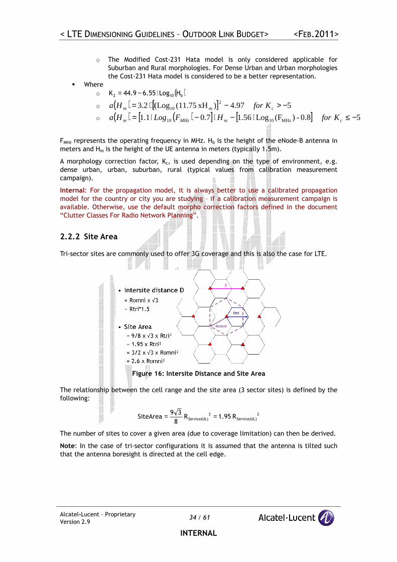
2.2.2 Site Area
Tri-sector sites are commonly used to offer 3G coverage and this is also the case for LTE.
Figure 16: Intersite Distance and Site Area
The relationship between the cell range and the site area (3 sector sites) is defined by the
following:
2
)Service(UL
2
)Service(UL R1.95R8
39SiteArea ==
The number of sites to cover a given area (due to coverage limitation) can then be derived.
Note: In the case of tri-sector configurations it is assumed that the antenna is tilted such
that the antenna boresight is directed at the cell edge.
< LTE DIMENSIONING GUIDELINES – OUTDOOR LINK BUDGET> <FEB.2011>
Alcatel-Lucent – Proprietary
Version 2.9 35 / 61
INTERNAL
2.3 Impact of RRH and TMA
2.3.1 RRH
Remote Radio Heads (RRH) are a popular solution that enables to separate the RF part of
the eNode-B and locate it physically close to the antenna, resulting lower feeder losses
between the eNode-B and the antenna (lower losses on UL, more effective radiated power
on the DL). Depending on where the RRH is located relative to the antenna, more or less
losses have to be considered in the uplink link budget:
� At least 0.5dB losses should be considered due to the jumper required between the
RRH and the antenna, applicable where the RRH is deployed very close to the
antenna,
� Higher losses should be considered if the RRH is installed farther from the antenna
(e.g. RRH at rooftop but still some non-zero length of feeder between the RRH and
the antenna).
The other parameters of the link budget are not modified.
2.3.2 TMA
Tower Mounted Amplifiers (TMA) (also called Mast Head Amplifiers (MHA) or Tower Top Low
Noise Amplifiers (TTLNA)) can be used to enhance the uplink coverage of eNode-Bs with
high feeder losses between the eNode-B and the antenna, allowing the required number of
sites to be minimized (in the case of coverage-limited scenarios but not for capacity-
limited scenarios) or allowing the reuse of incumbent 2G/3G sites to be maximized while
offering higher data rates than in 2G/3G.
For example, TMAs can be particularly beneficial if LTE is deployed in the 2.6GHz band,
while incumbent 2G/3G sites were deployed in a lower band (e.g. 2GHz or even 850 or
900MHz), this allows the uplink LTE cell range, affected by higher propagation losses at the
higher frequency, to be enhanced.
As for any active element inserted in the reception chain of an eNode-B, the impact of a
TMA on the link budget can be assessed by means of the Friis formula.
feederTMA
BeNode
TMA
feederTMAoverall
gg
1n
g
1nnn
⋅−+−+= − with 10
NF
element
element
10n = and 10
G
element
element
10g = ,
where NFfeeder = -Gfeeder = Feeder Losses. The typical TMA characteristics are NFTMA = 2dB,
GTMA = 12dB and Insertion Losses = 0.4dB
This has 2 key impacts on the link budget parameters:
� Compensation of the feeder losses,
� Reduction in the overall Noise Figure of the eNode-B.
However, TMA insertion losses of 0.4dB must be considered in the DL link budget.
The typical gain on the MAPL for a 3dB feeder loss is approximately 2.7dB, which
corresponds to 36% less sites, thanks to TMA usage. Note that such gains are only applicable
for scenarios where uplink coverage remains as the limitation (i.e. low traffic scenarios).
< LTE DIMENSIONING GUIDELINES – OUTDOOR LINK BUDGET> <FEB.2011>
Alcatel-Lucent – Proprietary
Version 2.9 36 / 61
INTERNAL
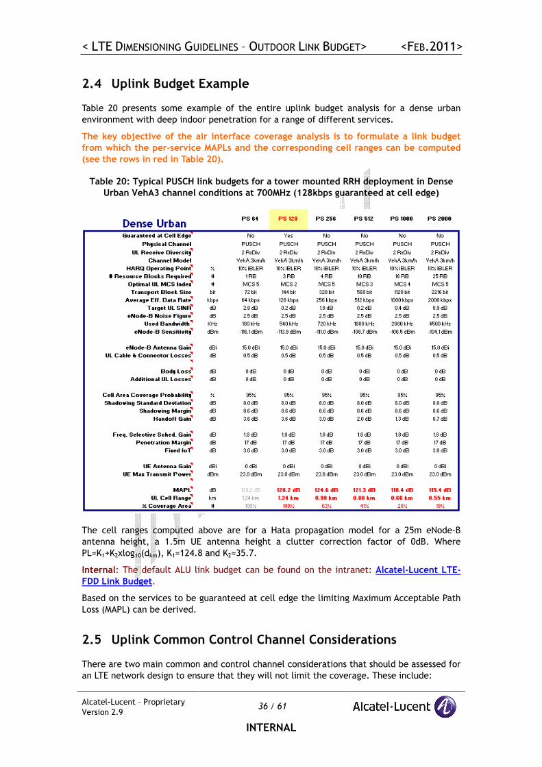
2.4 Uplink Budget Example
Table 20 presents some example of the entire uplink budget analysis for a dense urban
environment with deep indoor penetration for a range of different services.
The key objective of the air interface coverage analysis is to formulate a link budget
from which the per-service MAPLs and the corresponding cell ranges can be computed
(see the rows in red in Table 20).
Table 20: Typical PUSCH link budgets for a tower mounted RRH deployment in Dense
Urban VehA3 channel conditions at 700MHz (128kbps guaranteed at cell edge)
The cell ranges computed above are for a Hata propagation model for a 25m eNode-B
antenna height, a 1.5m UE antenna height a clutter correction factor of 0dB. Where
PL=K1+K2xlog10(dkm), K1=124.8 and K2=35.7.
Internal: The default ALU link budget can be found on the intranet: Alcatel-Lucent LTE-
FDD Link Budget.
Based on the services to be guaranteed at cell edge the limiting Maximum Acceptable Path
Loss (MAPL) can be derived.
2.5 Uplink Common Control Channel Considerations
There are two main common and control channel considerations that should be assessed for
an LTE network design to ensure that they will not limit the coverage. These include:
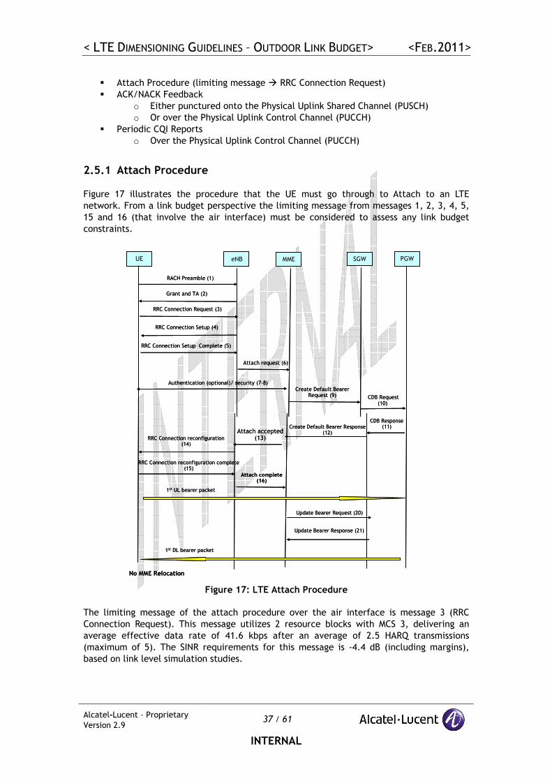
< LTE DIMENSIONING GUIDELINES – OUTDOOR LINK BUDGET> <FEB.2011>
Alcatel-Lucent – Proprietary
Version 2.9 37 / 61
INTERNAL
� Attach Procedure (limiting message � RRC Connection Request)
� ACK/NACK Feedback
o Either punctured onto the Physical Uplink Shared Channel (PUSCH)
o Or over the Physical Uplink Control Channel (PUCCH)
� Periodic CQI Reports
o Over the Physical Uplink Control Channel (PUCCH)
2.5.1 Attach Procedure
Figure 17 illustrates the procedure that the UE must go through to Attach to an LTE
network. From a link budget perspective the limiting message from messages 1, 2, 3, 4, 5,
15 and 16 (that involve the air interface) must be considered to assess any link budget
constraints.
eNBUE MME
RACH Preamble (1)
Grant and TA (2)
RRC Connection Request (3)
RRC Connection Setup (4)
RRC Connection Setup Complete (5)
SGW PGW
Attach request (6)
Authentication (optional)/ security (7-8)Create Default Bearer
Request (9) CDB Request (10)
Attach accepted (13)
Create Default Bearer Response (12)
CDB Response (11)
RRC Connection reconfiguration (14)
RRC Connection reconfiguration complete (15)
Attach complete (16)
No MME Relocation
1st UL bearer packet
Update Bearer Request (20)
Update Bearer Response (21)
1st DL bearer packet
Figure 17: LTE Attach Procedure
The limiting message of the attach procedure over the air interface is message 3 (RRC
Connection Request). This message utilizes 2 resource blocks with MCS 3, delivering an
average effective data rate of 41.6 kbps after an average of 2.5 HARQ transmissions
(maximum of 5). The SINR requirements for this message is -4.4 dB (including margins),
based on link level simulation studies.
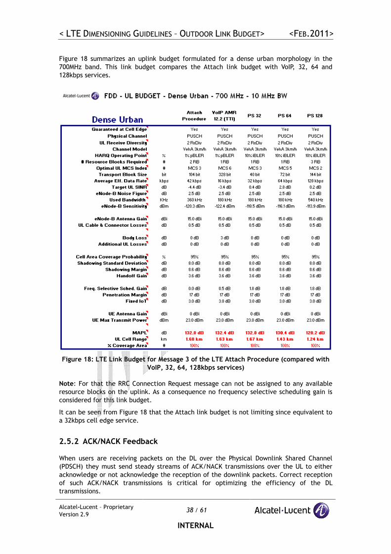
< LTE DIMENSIONING GUIDELINES – OUTDOOR LINK BUDGET> <FEB.2011>
Alcatel-Lucent – Proprietary
Version 2.9 38 / 61
INTERNAL
Figure 18 summarizes an uplink budget formulated for a dense urban morphology in the
700MHz band. This link budget compares the Attach link budget with VoIP, 32, 64 and
128kbps services.
Figure 18: LTE Link Budget for Message 3 of the LTE Attach Procedure (compared with
VoIP, 32, 64, 128kbps services)
Note: For that the RRC Connection Request message can not be assigned to any available
resource blocks on the uplink. As a consequence no frequency selective scheduling gain is
considered for this link budget.
It can be seen from Figure 18 that the Attach link budget is not limiting since equivalent to
a 32kbps cell edge service.
2.5.2 ACK/NACK Feedback
When users are receiving packets on the DL over the Physical Downlink Shared Channel
(PDSCH) they must send steady streams of ACK/NACK transmissions over the UL to either
acknowledge or not acknowledge the reception of the downlink packets. Correct reception
of such ACK/NACK transmissions is critical for optimizing the efficiency of the DL
transmissions.
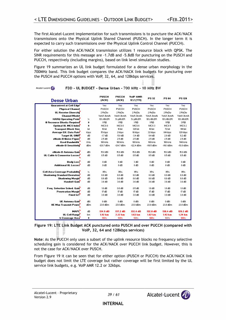
< LTE DIMENSIONING GUIDELINES – OUTDOOR LINK BUDGET> <FEB.2011>
Alcatel-Lucent – Proprietary
Version 2.9 39 / 61
INTERNAL
The first Alcatel-Lucent implementation for such transmissions is to puncture the ACK/NACK
transmissions onto the Physical Uplink Shared Channel (PUSCH). In the longer term it is
expected to carry such transmissions over the Physical Uplink Control Channel (PUCCH).
For either solution the ACK/NACK transmission utilizes 1 resource block with QPSK. The
SINR requirements for this message are -1.7dB and -5.8dB for puncturing on the PUSCH and
PUCCH, respectively (including margins), based on link level simulation studies.
Figure 19 summarizes an UL link budget formulated for a dense urban morphology in the
700MHz band. This link budget compares the ACK/NACK link budgets for puncturing over
the PUSCH and PUCCH options with VoIP, 32, 64, and 128kbps services.
Figure 19: LTE Link Budget ACK punctured onto PUSCH and over PUCCH (compared with
VoIP, 32, 64 and 128kbps services)
Note: As the PUCCH only uses a subset of the uplink resource blocks no frequency selective
scheduling gain is considered for the ACK/NACK over PUCCH link budget. However, this is
not the case for ACK/NACK over PUSCH.
From Figure 19 it can be seen that for either option (PUSCH or PUCCH) the ACK/NACK link
budget does not limit the LTE coverage but rather coverage will be first limited by the UL
service link budgets, e.g. VoIP AMR 12.2 or 32kbps.
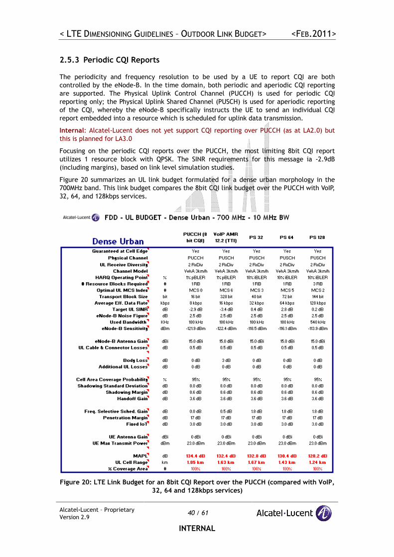
< LTE DIMENSIONING GUIDELINES – OUTDOOR LINK BUDGET> <FEB.2011>
Alcatel-Lucent – Proprietary
Version 2.9 40 / 61
INTERNAL
2.5.3 Periodic CQI Reports
The periodicity and frequency resolution to be used by a UE to report CQI are both
controlled by the eNode-B. In the time domain, both periodic and aperiodic CQI reporting
are supported. The Physical Uplink Control Channel (PUCCH) is used for periodic CQI
reporting only; the Physical Uplink Shared Channel (PUSCH) is used for aperiodic reporting
of the CQI, whereby the eNode-B specifically instructs the UE to send an individual CQI
report embedded into a resource which is scheduled for uplink data transmission.
Internal: Alcatel-Lucent does not yet support CQI reporting over PUCCH (as at LA2.0) but
this is planned for LA3.0
Focusing on the periodic CQI reports over the PUCCH, the most limiting 8bit CQI report
utilizes 1 resource block with QPSK. The SINR requirements for this message ia -2.9dB
(including margins), based on link level simulation studies.
Figure 20 summarizes an UL link budget formulated for a dense urban morphology in the
700MHz band. This link budget compares the 8bit CQI link budget over the PUCCH with VoIP,
32, 64, and 128kbps services.
Figure 20: LTE Link Budget for an 8bit CQI Report over the PUCCH (compared with VoIP,
32, 64 and 128kbps services)
< LTE DIMENSIONING GUIDELINES – OUTDOOR LINK BUDGET> <FEB.2011>
Alcatel-Lucent – Proprietary
Version 2.9 41 / 61
INTERNAL
Note: As the PUCCH only uses a subset of the uplink resource blocks no frequency selective
scheduling gain is considered for the 8bit CQI report over PUCCH link budget.
From Figure 20 it can be seen that the 8bit CQI link budget over the PUCCH does not limit
the LTE coverage but rather coverage will be first limited by the UL service link budgets,
e.g. VoIP AMR 12.2 or 32kbps.
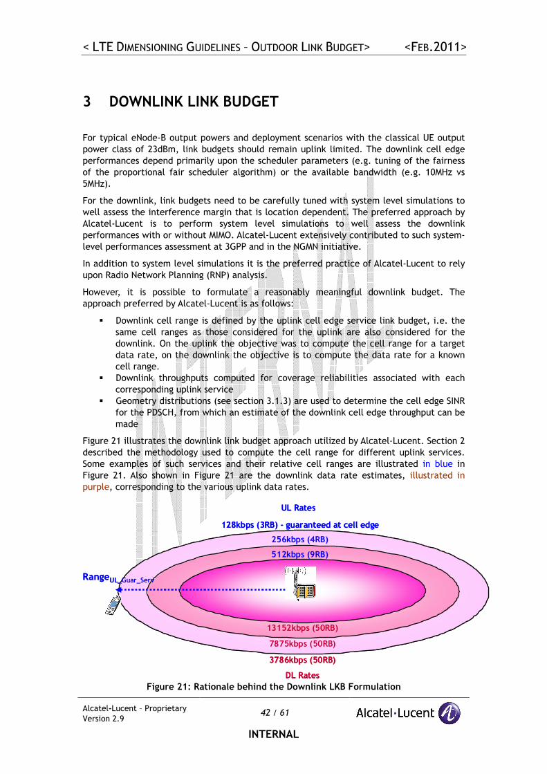
< LTE DIMENSIONING GUIDELINES – OUTDOOR LINK BUDGET> <FEB.2011>
Alcatel-Lucent – Proprietary
Version 2.9 42 / 61
INTERNAL
3 DOWNLINK LINK BUDGET
For typical eNode-B output powers and deployment scenarios with the classical UE output
power class of 23dBm, link budgets should remain uplink limited. The downlink cell edge
performances depend primarily upon the scheduler parameters (e.g. tuning of the fairness
of the proportional fair scheduler algorithm) or the available bandwidth (e.g. 10MHz vs
5MHz).
For the downlink, link budgets need to be carefully tuned with system level simulations to
well assess the interference margin that is location dependent. The preferred approach by
Alcatel-Lucent is to perform system level simulations to well assess the downlink
performances with or without MIMO. Alcatel-Lucent extensively contributed to such system-
level performances assessment at 3GPP and in the NGMN initiative.
In addition to system level simulations it is the preferred practice of Alcatel-Lucent to rely
upon Radio Network Planning (RNP) analysis.
However, it is possible to formulate a reasonably meaningful downlink budget. The
approach preferred by Alcatel-Lucent is as follows:
� Downlink cell range is defined by the uplink cell edge service link budget, i.e. the
same cell ranges as those considered for the uplink are also considered for the
downlink. On the uplink the objective was to compute the cell range for a target
data rate, on the downlink the objective is to compute the data rate for a known
cell range.
� Downlink throughputs computed for coverage reliabilities associated with each
corresponding uplink service
� Geometry distributions (see section 3.1.3) are used to determine the cell edge SINR
for the PDSCH, from which an estimate of the downlink cell edge throughput can be
made
Figure 21 illustrates the downlink link budget approach utilized by Alcatel-Lucent. Section 2
described the methodology used to compute the cell range for different uplink services.
Some examples of such services and their relative cell ranges are illustrated in blue in
Figure 21. Also shown in Figure 21 are the downlink data rate estimates, illustrated in
purple, corresponding to the various uplink data rates.
RangeUL_Guar_Serv
128kbps (3RB) - guaranteed at cell edge
256kbps (4RB)
512kbps (9RB)
UL Rates
DL Rates
7875kbps (50RB)
13152kbps (50RB)
3786kbps (50RB)
RangeUL_Guar_Serv
128kbps (3RB) - guaranteed at cell edge
256kbps (4RB)
512kbps (9RB)
UL Rates
DL Rates
7875kbps (50RB)
13152kbps (50RB)
3786kbps (50RB)
Figure 21: Rationale behind the Downlink LKB Formulation
< LTE DIMENSIONING GUIDELINES – OUTDOOR LINK BUDGET> <FEB.2011>
Alcatel-Lucent – Proprietary
Version 2.9 43 / 61
INTERNAL
The example shown in Figure 21 is for an urban morphology, indoor 0dBi omni UE
configuration, cell range fixed for uplink 128kbps, 50% adjacent cell downlink resource
block loading, no TMA, 700MHz and 10MHz bandwidth. This example illustrates the concept
behind downlink link budget approach that is described in this section.
Note: The diagram shown in Figure 21 is not to scale and does not include all rates.
3.1 Downlink Budget Parameters
3.1.1 SINR
One of the measures of quality used on the downlink is the SINR. There are a number of
important channels for which the SINR is of interest, these include:
� SINRPDSCH
� SINRPDCCH
� SINRDLRS
Of the above, the SINRPDSCH is the most commonly referenced downlink SINR metric.
Note: There is no consistent standard or industry defined measure of SINRPDSCH exists that is
a completely unambiguous and can be used as a concise reference measure of downlink
signal quality in the field.
For example, the SINRPDSCH can be quantified both with and without inclusion of a
combining gain at the UE (the default for Alcatel-Lucent is to incorporate such a combining
gain). While Alcatel-Lucent link level performances are quantified in terms of the SINRPDSCH,
the reference to be used, measured and validated in the field is the RSRQ (see section
3.1.2), which is more unambiguously defined.
Unlike the uplink, the observed downlink SINR performances are dependent upon the UE
location, i.e. the signal to interference plus noise ratio for the PDSCH, PDCCH or DLRS
channels, SINRChannel_Des, is dependent on the user location. Thus, for a given UE location,
SINRChannel_Des, for a number of transmit paths, PathDL, is given by:
(DL)j(DL)
DL(DL) Desj_Channel_
sChannel_DeNI
PathsCINRS
+⋅
= ,
where Channel_Des is the desired channel for the SINR computation. This can be either
PDSCH, PDCCH or DLRS.
Note: PathsDL = 1 when computing SINRDLRS as the DLRS is not transmitted on the same RE
from all transmit paths.
The worst performances will be experienced when the UE is at cell edge far from the
eNode-B. The relationship between the SINRPDSCH, and downlink throughput is discussed in
more detail in section 3.1.5.
Cj_Channel_Des (DL) is the power of the considered channel, PDSCH, PDCCH or DLRS, received at
the UE located at the uplink service cell range, RService(UL), per Resource Element (RE) from
the UE’s serving eNode-B, that is transmitting with its maximal power and is given by:
ChanneldBmj_DLRS(DL)dBm(DL) Desj_Channel_ OffsetCC +=
( ) ( )( )
dBdBdBdBdB
dBdBdBdB
HOShadowingRxRxnPenetratio
Body)UL(ServicenPropagatioTxTxDLRSdBmj_DLRS(DL)
GainMarginLossGaininargM
LossRLossesLossGainEPREC
+−−+−
−−−+=
< LTE DIMENSIONING GUIDELINES – OUTDOOR LINK BUDGET> <FEB.2011>
Alcatel-Lucent – Proprietary
Version 2.9 44 / 61
INTERNAL
where
� EPREDLRS is the Energy Per Resource Element for the reference symbol (see Section
3.1.7)
� OffsetPDSCH / PDCCH / DLRS is the margin by which PDSCH, PDCCH and DLRS RE’s are
offset in power from the EPREDLRS. OffsetDLRS is by definition always equal to 0dB.
OffsetPDCCH is driven by dynamic PDCCH power control.
� GainTx and LossTx, represent the gains and losses at the transmitter side such as the
eNode-B antenna gain and the feeder losses between the eNode-B and the antenna,
� GainRx and LossRx, the gains and losses at the receiver side such as UE antenna gain,
� LossBody is the body loss induced by the users proximity to the UE, typically 3dB
body losses are considered for voice services and 0 dB for data services (handset
position is far from the head when using data services),
� MarginPenetration is the loss (in dB) induced by buildings, windows or vehicles
according to the penetration coverage objective (deep or light indoor, outdoor)
(see Section 2.1.11),
� The downlink MAPL, MAPL(DL)dB, that corresponds to an uplink service cell range,
RService(UL) (as computed in section 2.2), is dependent upon the propagation model
differences (K1(DL) & K2(DL)) due to the frequency duplex difference between uplink
and downlink,
� MarginShadowing is a margin that compensates for the slow variability in mean path
loss about that predicted using the propagation model, e.g. Hata (see section 0)
� GainHO is a handoff gain or best server selection gain that models the benefits due
to the ability to reselect to the best available serving site at any given location (see
section 0)
( ))Service(UL2(DL)1(DL)nPropagatio RlogKKLossesdB
+= .
Ij(DL), is the average received interfering power at the UE from all adjacent cells per RE.
Averaging is based upon the average number of RE allocated to the various interfering
channels. The channels considered as sources of interference, Channel_Int, are detailed in
section 3.1.3, these can include a combination of the PDSCH, RS, PDCCH, SCH, BCH, PCFICH
and PHICH. The average number of RE elements per TTI assigned to each channel type is
detailed in Section 3.1.6.
( )SINR_ShadPercentileDL
PHICH(DL)&j_PCFICHj_BCH(DL)j_SCH(DL)j_DLRS(DL)
DLAvg)j_PDCCH(DLAvg)j_PDSCH(DL
dBmj(DL) inargMGeometry -PathsIIII
LoadingIII
AvgAvgAvgAvg
+⋅
+++
+⋅+=
where
� Ij_Channel_Int(DL) is the average interference contribution due to RE’s allocated to the
various interfering channels (where Channel_Int can be PDSCH, PDCCH, SCH, BCH
and PCFICH & PHICH) and is given by (Note: power offset for PDCCH interferences
is assumed to be null to account for dynamic PDCCH power control):
( )TTI_Total
TTI_hannelCInt_hannelC
ChanneldBmj_RS(DL)AvgInt(DL)j_Channel_RE
REConsideredOffsetCI
⋅⋅+= ,
� Ij_RS(DL) is the average interference contribution due to RE’s allocated to RS’s and is
given by (Note: The 3rd and 4th antennas, if present, only transmit the RS on half
the number of RE’s as the 1st two antennas):
( )TTI_Total
TTI_DLRSInt_DLRS
DLj_RS(DL)j_RS(DL)RE
REConsidered1Else75.0Then,4PathsIfCI
Avg
⋅⋅=⋅= ,
< LTE DIMENSIONING GUIDELINES – OUTDOOR LINK BUDGET> <FEB.2011>
Alcatel-Lucent – Proprietary
Version 2.9 45 / 61
INTERNAL
� RETotal_TTI, is the sum of the RE for the considered interfering channels and is given
by (where ConsideredChannels_Int for PDSCH, DLRS, PDCCH, SCH, BCH and PCFICH &
PHICH is defined in section 3.1.3 and depends upon the considered Channel_Des):
∑ ⋅=ChannelsAll
TTI_ChannelInt_ChannelTTI_Total REConsideredRE
� LoadingDL is the assumed average resource blocking loading of adjacent cells on the
downlink. Note: It is assumed that the interference due to both PDSCH and PDCCH
from adjacent cells will be reduced with reduced average RB loading.
� GeometryReliability, represents the downlink geometry that corresponds to the UL cell
range, RService(UL) (discussed in more detailed in section 3.1.3),
� MarginShad_SINR is the shadowing margin applied to the SINR distribution to account
for the fact that the desired and interfering signals are not perfectly correlated
with each other (see section 0)
The thermal noise for a single subcarrier is given by:
( )SC10UEthdBm)DL( WLog10FNN ⋅++=
where
� Nth is the thermal noise density (-174dBm/Hz),
� FUE is the noise figure of the UE receiver (8dB by default),
� WSC is the bandwidth used by one subcarrier, each of a 15kHz bandwidth.
Internal: Note that currently there is no consideration of any frequency selective
scheduling benefits in the downlink budget as there is in the uplink (see section 2.1.10).
This does not mean such gains are not realized in the field on the downlink, but rather that
such gains are not yet accounted for in the current downlink budget. This may be addressed
in future link budget updates.
3.1.2 RSRQ
While, SINRPDSCH, is a meaningful measure of the cell edge quality (see section 3.1.1), this is
not a measure that is standardized by 3GPP and as such is somewhat open to interpretation
when it comes to measurement in the field, i.e. whether a power combining gain is
accounted for in the computation of SINR. The standardized measure of the downlink
quality is RSRQ (Reference Symbol Receive Quality) and is given by:
TotalRB10)Service(UL RSSI)N(log10 SRPRRSRQ −⋅+=
where
� RSRP is the Reference Signal Received Power at the UE from its serving cell and is
given by Cj_DLRS(DL) (see above)
� NRB is the maximum number of RB’s for the consider carrier bandwidth
� RSSITotal is the total received power at the UE from its serving cell and all adjacent
cells across the entire bandwidth and is given by:
( ) RBRB)DL()DL(jCell_OwnTotal NsSubCarrierNISSIRRSSI ⋅⋅++=
� SubCarriersRB is the number of sub carries per RB, this is defined by the standards
to be 12 sub-carriers per RB
� RSSIOwn_Cell is the average power received at the UE from its serving cell per RE. The
averaging is based upon the average number of RE allocated to the various
interfering channels (see Section 3.1.6 for details of the RE distribution) and is
given by:
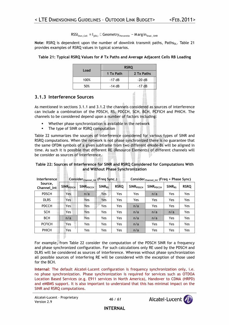
< LTE DIMENSIONING GUIDELINES – OUTDOOR LINK BUDGET> <FEB.2011>
Alcatel-Lucent – Proprietary
Version 2.9 46 / 61
INTERNAL
SINR_ShadPercentile)DL(jOwn_Cell inargMGeometry IRSSI −+=
Note: RSRQ is dependent upon the number of downlink transmit paths, PathsDL. Table 21
provides examples of RSRQ values in typical scenarios.
Table 21: Typical RSRQ Values for # Tx Paths and Average Adjacent Cells RB Loading
RSRQ Load
1 Tx Path 2 Tx Paths
100% -17 dB -20 dB
50% -14 dB -17 dB
3.1.3 Interference Sources
As mentioned in sections 3.1.1 and 3.1.2 the channels considered as sources of interference
can include a combination of the PDSCH, RS, PDCCH, SCH, BCH, PCFICH and PHICH. The
channels to be considered depend upon a number of factors including:
� Whether phase synchronization is available in the network
� The type of SINR or RSRQ computation
Table 22 summarizes the sources of interference considered for various types of SINR and
RSRQ computations. When the network is not phase synchronized there is no guarantee that
the same OFDM symbols of a given subframe from two different eNode-Bs will be aligned in
time. As such it is possible that different RE (Resource Elements) of different channels will
be consider as sources of interference.
Table 22: Sources of Interference for SINR and RSRQ Considered for Computations With
and Without Phase Synchronization
ConsiderChannel_Int (Freq Sync.) ConsiderChannel_Int (Freq + Phase Sync) Interference
Source,
Channel_Int SINRPDSCH SINRPDCCH SINRRS RSRQ SINRPDSCH SINRPDCCH SINRRS RSRQ
PDSCH Yes n/a Yes Yes Yes n/a Yes Yes
DLRS Yes Yes Yes Yes Yes Yes Yes Yes
PDCCH Yes Yes Yes Yes n/a Yes Yes Yes
SCH Yes Yes Yes Yes n/a n/a n/a Yes
BCH n/a Yes Yes Yes n/a n/a Yes Yes
PCFICH Yes Yes Yes Yes n/a Yes Yes Yes
PHICH Yes Yes Yes Yes n/a Yes Yes Yes
For example, from Table 22 consider the computation of the PDSCH SINR for a frequency
and phase synchronized configuration. For such calculations only RE used by the PDSCH and
DLRS will be considered as sources of interference. Whereas without phase synchronization
all possible sources of interfering RE will be considered with the exception of those used
for the BCH.
Internal: The default Alcatel-Lucent configuration is frequency synchronization only, i.e.
no phase synchronization. Phase synchronization is required for services such as OTDOA
Location Based Services (e.g. E911 services in North America), Handover to CDMA (HRPD)
and eMBMS support. It is also important to understand that this has minimal impact on the
SINR and RSRQ computations.
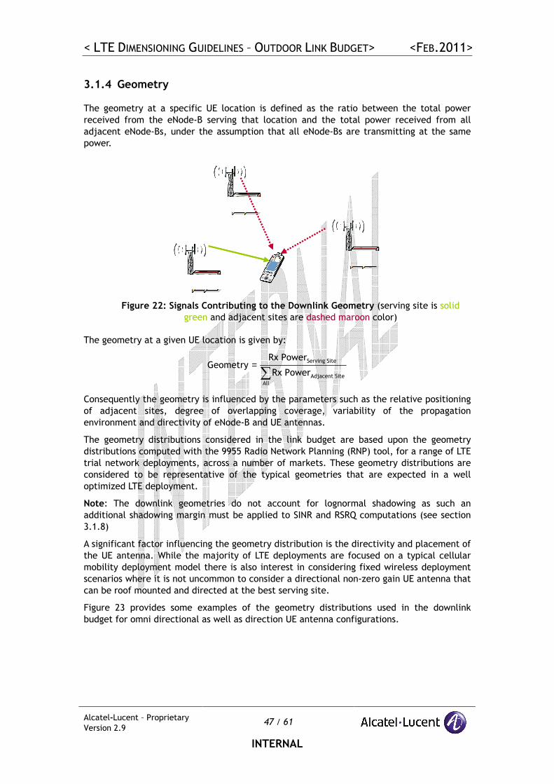
< LTE DIMENSIONING GUIDELINES – OUTDOOR LINK BUDGET> <FEB.2011>
Alcatel-Lucent – Proprietary
Version 2.9 47 / 61
INTERNAL
3.1.4 Geometry
The geometry at a specific UE location is defined as the ratio between the total power
received from the eNode-B serving that location and the total power received from all
adjacent eNode-Bs, under the assumption that all eNode-Bs are transmitting at the same
power.
Figure 22: Signals Contributing to the Downlink Geometry (serving site is solid
green and adjacent sites are dashed maroon color)
The geometry at a given UE location is given by:
∑=
All
SiteAdjacent
SiteServing
PowerRx
PowerRxGeometry
Consequently the geometry is influenced by the parameters such as the relative positioning
of adjacent sites, degree of overlapping coverage, variability of the propagation
environment and directivity of eNode-B and UE antennas.
The geometry distributions considered in the link budget are based upon the geometry
distributions computed with the 9955 Radio Network Planning (RNP) tool, for a range of LTE
trial network deployments, across a number of markets. These geometry distributions are
considered to be representative of the typical geometries that are expected in a well
optimized LTE deployment.
Note: The downlink geometries do not account for lognormal shadowing as such an
additional shadowing margin must be applied to SINR and RSRQ computations (see section
3.1.8)
A significant factor influencing the geometry distribution is the directivity and placement of
the UE antenna. While the majority of LTE deployments are focused on a typical cellular
mobility deployment model there is also interest in considering fixed wireless deployment
scenarios where it is not uncommon to consider a directional non-zero gain UE antenna that
can be roof mounted and directed at the best serving site.
Figure 23 provides some examples of the geometry distributions used in the downlink
budget for omni directional as well as direction UE antenna configurations.
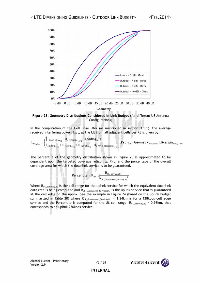
< LTE DIMENSIONING GUIDELINES – OUTDOOR LINK BUDGET> <FEB.2011>
Alcatel-Lucent – Proprietary
Version 2.9 48 / 61
INTERNAL
0%
10%
20%
30%
40%
50%
60%
70%
80%
90%
100%
-5 dB 0 dB 5 dB 10 dB 15 dB 20 dB 25 dB 30 dB 35 dB 40 dB
Geometry
Indoor - 0 dBi - Omni
Outdoor - 4 dBi - Direc.
Outdoor - 8 dBi - Direc.
Outdoor - 10 dBi - Direc.
Figure 23: Geometry Distributions Considered in Link Budget (for different UE Antenna
Configurations)
In the computation of the Cell Edge SINR (as mentioned in section 3.1.1), the average
received interfering power, Ij(DL), at the UE from all adjacent cells per RE is given by:
( )SINR_ShadPercentileDL
PHICH(DL)&j_PCFICHj_BCH(DL)j_SCH(DL)j_DLRS(DL)
DLAvg)j_PDCCH(DLAvg)j_PDSCH(DL
dBmj(DL) inargMGeometry -PathsIIII
LoadingIII
AvgAvgAvgAvg
+⋅
+++
+⋅+=
The percentile of the geometry distribution shown in Figure 23 is approximated to be
dependent upon the targeted coverage reliability, PCov, and the percentage of the overall
coverage area for which the downlink service is to be guaranteed.
2
e(UL)eed_ServicUL_Guarant
2
(UL)UL_Service
CovR
RPPercentile ⋅=
Where RUL_Service(UL) is the cell range for the uplink service for which the equivalent downlink
data rate is being computed and RUL_Guaranteed_Service(UL) is the uplink service that is guaranteed
at the cell edge on the uplink. See the example in Figure 24 (based on the uplink budget
summarized in Table 20) where RUL_Guaranteed_Service(UL) = 1.24km is for a 128kbps cell edge
service and the Percentile is computed for the UL cell range, RUL_Service(UL) = 0.98km, that
corresponds to an uplink 256kbps service.
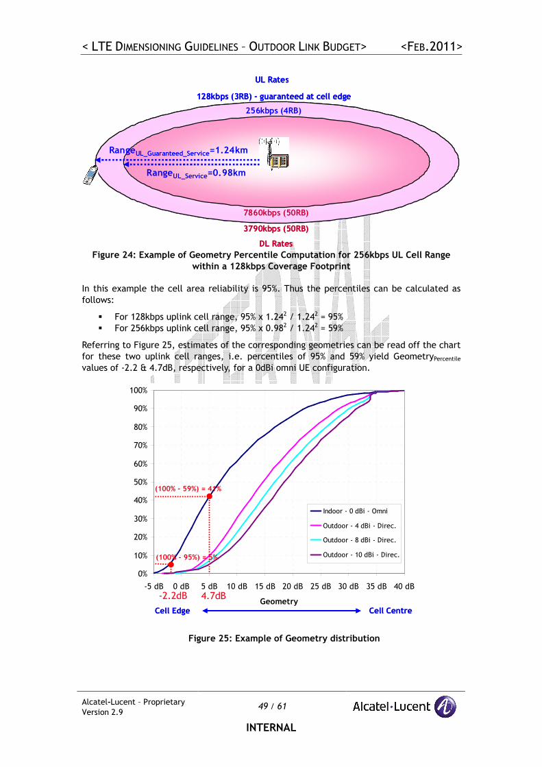
< LTE DIMENSIONING GUIDELINES – OUTDOOR LINK BUDGET> <FEB.2011>
Alcatel-Lucent – Proprietary
Version 2.9 49 / 61
INTERNAL
RangeUL_Guaranteed_Service=1.24km
128kbps (3RB) - guaranteed at cell edge
256kbps (4RB)
UL Rates
DL Rates
7860kbps (50RB)
3790kbps (50RB)
RangeUL_Service=0.98km
RangeUL_Guaranteed_Service=1.24km
128kbps (3RB) - guaranteed at cell edge
256kbps (4RB)
UL Rates
DL Rates
7860kbps (50RB)
3790kbps (50RB)
RangeUL_Service=0.98km
Figure 24: Example of Geometry Percentile Computation for 256kbps UL Cell Range
within a 128kbps Coverage Footprint
In this example the cell area reliability is 95%. Thus the percentiles can be calculated as
follows:
� For 128kbps uplink cell range, 95% x 1.242 / 1.242 = 95%
� For 256kbps uplink cell range, 95% x 0.982 / 1.242 = 59%
Referring to Figure 25, estimates of the corresponding geometries can be read off the chart
for these two uplink cell ranges, i.e. percentiles of 95% and 59% yield GeometryPercentile
values of -2.2 & 4.7dB, respectively, for a 0dBi omni UE configuration.
0%
10%
20%
30%
40%
50%
60%
70%
80%
90%
100%
-5 dB 0 dB 5 dB 10 dB 15 dB 20 dB 25 dB 30 dB 35 dB 40 dB
Geometry
Indoor - 0 dBi - Omni
Outdoor - 4 dBi - Direc.
Outdoor - 8 dBi - Direc.
Outdoor - 10 dBi - Direc.(100% - 95%) = 5%
-2.2dB
(100% - 59%) = 41%
4.7dB
Cell Edge Cell Centre
0%
10%
20%
30%
40%
50%
60%
70%
80%
90%
100%
-5 dB 0 dB 5 dB 10 dB 15 dB 20 dB 25 dB 30 dB 35 dB 40 dB
Geometry
Indoor - 0 dBi - Omni
Outdoor - 4 dBi - Direc.
Outdoor - 8 dBi - Direc.
Outdoor - 10 dBi - Direc.(100% - 95%) = 5%
-2.2dB
(100% - 59%) = 41%
4.7dB
Cell Edge Cell Centre
Figure 25: Example of Geometry distribution
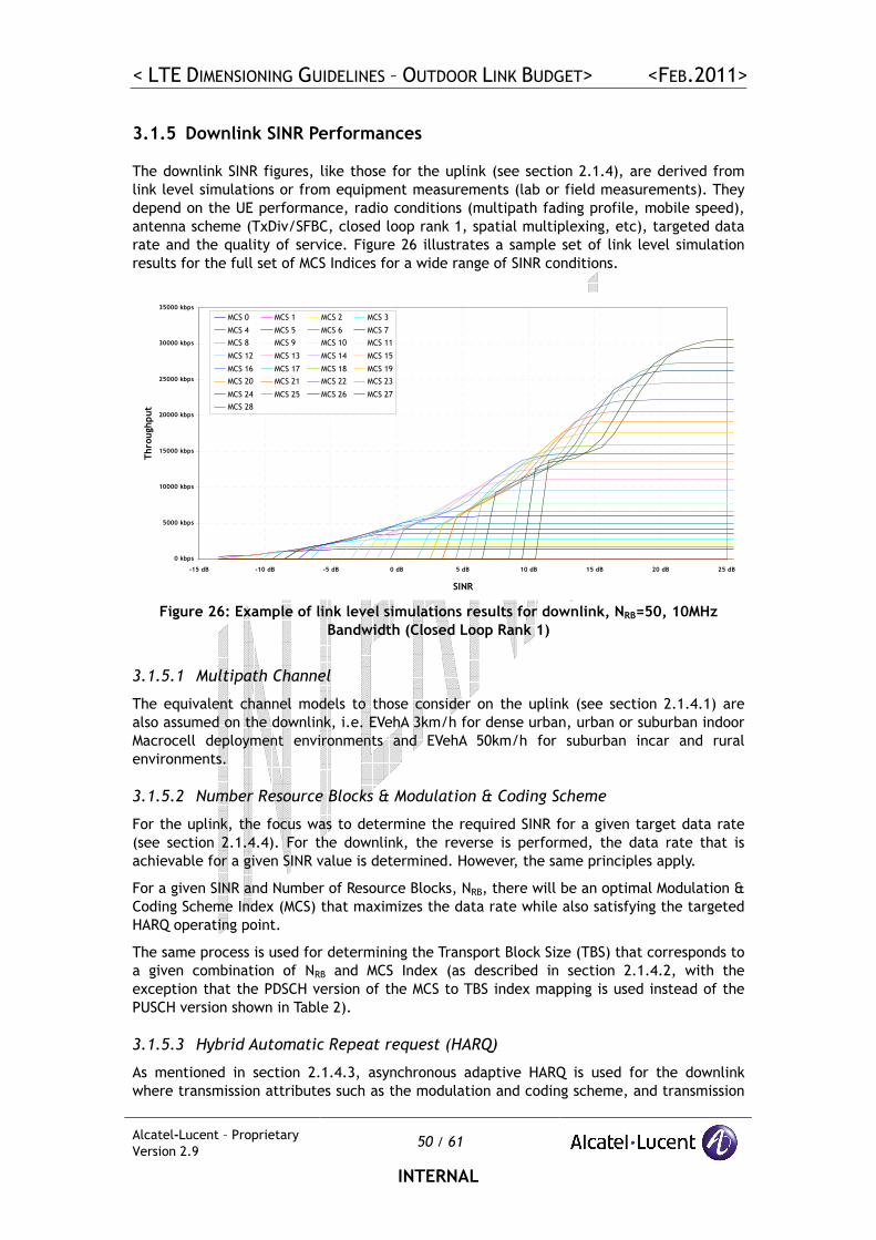
< LTE DIMENSIONING GUIDELINES – OUTDOOR LINK BUDGET> <FEB.2011>
Alcatel-Lucent – Proprietary
Version 2.9 50 / 61
INTERNAL
3.1.5 Downlink SINR Performances
The downlink SINR figures, like those for the uplink (see section 2.1.4), are derived from
link level simulations or from equipment measurements (lab or field measurements). They
depend on the UE performance, radio conditions (multipath fading profile, mobile speed),
antenna scheme (TxDiv/SFBC, closed loop rank 1, spatial multiplexing, etc), targeted data
rate and the quality of service. Figure 26 illustrates a sample set of link level simulation
results for the full set of MCS Indices for a wide range of SINR conditions.
0 kbps
5000 kbps
10000 kbps
15000 kbps
20000 kbps
25000 kbps
30000 kbps
35000 kbps
-15 dB -10 dB -5 dB 0 dB 5 dB 10 dB 15 dB 20 dB 25 dB
SINR
Throughput
MCS 0 MCS 1 MCS 2 MCS 3
MCS 4 MCS 5 MCS 6 MCS 7
MCS 8 MCS 9 MCS 10 MCS 11
MCS 12 MCS 13 MCS 14 MCS 15
MCS 16 MCS 17 MCS 18 MCS 19
MCS 20 MCS 21 MCS 22 MCS 23
MCS 24 MCS 25 MCS 26 MCS 27
MCS 28
Figure 26: Example of link level simulations results for downlink, NRB=50, 10MHz
Bandwidth (Closed Loop Rank 1)
3.1.5.1 Multipath Channel
The equivalent channel models to those consider on the uplink (see section 2.1.4.1) are
also assumed on the downlink, i.e. EVehA 3km/h for dense urban, urban or suburban indoor
Macrocell deployment environments and EVehA 50km/h for suburban incar and rural
environments.
3.1.5.2 Number Resource Blocks & Modulation & Coding Scheme
For the uplink, the focus was to determine the required SINR for a given target data rate
(see section 2.1.4.4). For the downlink, the reverse is performed, the data rate that is
achievable for a given SINR value is determined. However, the same principles apply.
For a given SINR and Number of Resource Blocks, NRB, there will be an optimal Modulation &
Coding Scheme Index (MCS) that maximizes the data rate while also satisfying the targeted
HARQ operating point.
The same process is used for determining the Transport Block Size (TBS) that corresponds to
a given combination of NRB and MCS Index (as described in section 2.1.4.2, with the
exception that the PDSCH version of the MCS to TBS index mapping is used instead of the
PUSCH version shown in Table 2).
3.1.5.3 Hybrid Automatic Repeat request (HARQ)
As mentioned in section 2.1.4.3, asynchronous adaptive HARQ is used for the downlink
where transmission attributes such as the modulation and coding scheme, and transmission
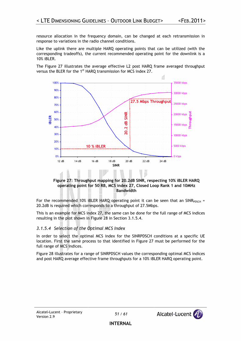
< LTE DIMENSIONING GUIDELINES – OUTDOOR LINK BUDGET> <FEB.2011>
Alcatel-Lucent – Proprietary
Version 2.9 51 / 61
INTERNAL
resource allocation in the frequency domain, can be changed at each retransmission in
response to variations in the radio channel conditions.
Like the uplink there are multiple HARQ operating points that can be utilized (with the
corresponding tradeoffs), the current recommended operating point for the downlink is a
10% iBLER.
The Figure 27 illustrates the average effective L2 post HARQ frame averaged throughput
versus the BLER for the 1st HARQ transmission for MCS index 27.
0%
10%
20%
30%
40%
50%
60%
70%
80%
90%
100%
12 dB 14 dB 16 dB 18 dB 20 dB 22 dB 24 dB
SINR
iBLER
0 kbps
5000 kbps
10000 kbps
15000 kbps
20000 kbps
25000 kbps
30000 kbps
35000 kbps
Through
put
10 % iBLER
20.2 dB SINR
27.5 Mbps Throughput
0%
10%
20%
30%
40%
50%
60%
70%
80%
90%
100%
12 dB 14 dB 16 dB 18 dB 20 dB 22 dB 24 dB
SINR
iBLER
0 kbps
5000 kbps
10000 kbps
15000 kbps
20000 kbps
25000 kbps
30000 kbps
35000 kbps
Through
put
10 % iBLER
20.2 dB SINR
27.5 Mbps Throughput
Figure 27: Throughput mapping for 20.2dB SINR, respecting 10% iBLER HARQ
operating point for 50 RB, MCS index 27, Closed Loop Rank 1 and 10MHz
Bandwidth
For the recommended 10% iBLER HARQ operating point it can be seen that an SINRPDSCH =
20.2dB is required which corresponds to a throughput of 27.5Mbps.
This is an example for MCS index 27, the same can be done for the full range of MCS indices
resulting in the plot shown in Figure 28 in Section 3.1.5.4.
3.1.5.4 Selection of the Optimal MCS Index
In order to select the optimal MCS index for the SINRPDSCH conditions at a specific UE
location. First the same process to that identified in Figure 27 must be performed for the
full range of MCS indices.
Figure 28 illustrates for a range of SINRPDSCH values the corresponding optimal MCS indices
and post HARQ average effective frame throughputs for a 10% iBLER HARQ operating point.
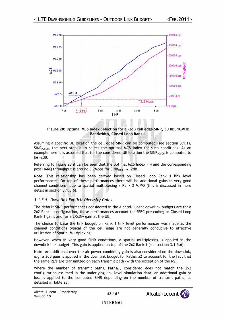
< LTE DIMENSIONING GUIDELINES – OUTDOOR LINK BUDGET> <FEB.2011>
Alcatel-Lucent – Proprietary
Version 2.9 52 / 61
INTERNAL
MCS 0
MCS 5
MCS 10
MCS 15
MCS 20
MCS 25
MCS 30
-7 dB -2 dB 3 dB 8 dB 13 dB 18 dB
SINR
MCS
0 kbps
5000 kbps
10000 kbps
15000 kbps
20000 kbps
25000 kbps
30000 kbps
35000 kbps
Throughput
˜ 3.2 Mbps
MCS 4
MCS 0
MCS 5
MCS 10
MCS 15
MCS 20
MCS 25
MCS 30
-7 dB -2 dB 3 dB 8 dB 13 dB 18 dB
SINR
MCS
0 kbps
5000 kbps
10000 kbps
15000 kbps
20000 kbps
25000 kbps
30000 kbps
35000 kbps
Throughput
˜ 3.2 Mbps
MCS 4
Figure 28: Optimal MCS Index Selection for a -2dB cell edge SINR, 50 RB, 10MHz
Bandwidth, Closed Loop Rank 1
Assuming a specific UE location the cell edge SINR can be computed (see section 3.1.1),
SINRPDSCH, the next step is to select the optimal MCS index for such conditions. As an
example here it is assumed that for the considered UE location the SINRPDSCH is computed to
be -2dB.
Referring to Figure 28 it can be seen that the optimal MCS Index = 4 and the corresponding
post HARQ throughput is around 3.2Mbps for SINRPDSCH = -2dB.
Note: This relationship has been derived based on Closed Loop Rank 1 link level
performances. On top of these performances there will be additional gains in very good
channel conditions, due to spatial multiplexing / Rank 2 MIMO (this is discussed in more
detail in section 3.1.5.6).
3.1.5.5 Downlink Explicit Diversity Gains
The default SINR performances considered in the Alcatel-Lucent downlink budgets are for a
2x2 Rank 1 configuration, these performances account for SFBC pre-coding or Closed Loop
Rank 1 gains and for a 2RxDiv gain at the UE.
The choice to base the link budget on Rank 1 link level performances was made as the
channel conditions typical of the cell edge are not generally conducive to effective
utilization of Spatial Multiplexing.
However, when in very good SINR conditions, a spatial multiplexing is applied in the
downlink link budget. This gain is applied on top of the 2x2 Rank 1 (see section 3.1.5.6).
Note: An additional over the air power combining gain is also considered on the downlink,
e.g. a 3dB gain is applied in the downlink budget for PathsDL≥2 to account for the fact that
the same RE’s are transmitted on each transmit path (with the exception of the RS).
Where the number of transmit paths, PathsDL, considered does not match the 2x2
configuration assumed in the underlying link level simulation data, an additional gain or
loss is applied to the computed SINR depending on the number of transmit paths, as
detailed in Table 23:
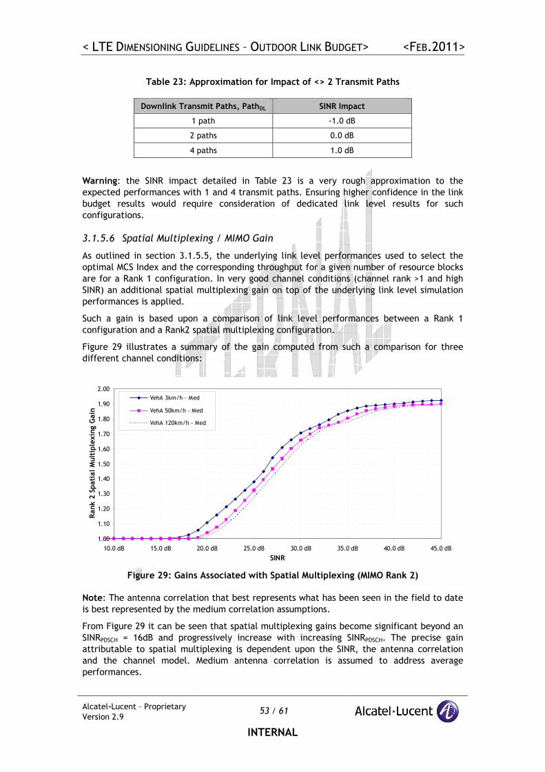
< LTE DIMENSIONING GUIDELINES – OUTDOOR LINK BUDGET> <FEB.2011>
Alcatel-Lucent – Proprietary
Version 2.9 53 / 61
INTERNAL
Table 23: Approximation for Impact of <> 2 Transmit Paths
Downlink Transmit Paths, PathDL SINR Impact
1 path -1.0 dB
2 paths 0.0 dB
4 paths 1.0 dB
Warning: the SINR impact detailed in Table 23 is a very rough approximation to the
expected performances with 1 and 4 transmit paths. Ensuring higher confidence in the link
budget results would require consideration of dedicated link level results for such
configurations.
3.1.5.6 Spatial Multiplexing / MIMO Gain
As outlined in section 3.1.5.5, the underlying link level performances used to select the
optimal MCS Index and the corresponding throughput for a given number of resource blocks
are for a Rank 1 configuration. In very good channel conditions (channel rank >1 and high
SINR) an additional spatial multiplexing gain on top of the underlying link level simulation
performances is applied.
Such a gain is based upon a comparison of link level performances between a Rank 1
configuration and a Rank2 spatial multiplexing configuration.
Figure 29 illustrates a summary of the gain computed from such a comparison for three
different channel conditions:
1.00
1.10
1.20
1.30
1.40
1.50
1.60
1.70
1.80
1.90
2.00
10.0 dB 15.0 dB 20.0 dB 25.0 dB 30.0 dB 35.0 dB 40.0 dB 45.0 dB
SINR
Rank 2 Spatial Multiplexing Gain
VehA 3km/h - Med
VehA 50km/h - Med
VehA 120km/h - Med
Figure 29: Gains Associated with Spatial Multiplexing (MIMO Rank 2)
Note: The antenna correlation that best represents what has been seen in the field to date
is best represented by the medium correlation assumptions.
From Figure 29 it can be seen that spatial multiplexing gains become significant beyond an
SINRPDSCH = 16dB and progressively increase with increasing SINRPDSCH. The precise gain
attributable to spatial multiplexing is dependent upon the SINR, the antenna correlation
and the channel model. Medium antenna correlation is assumed to address average
performances.
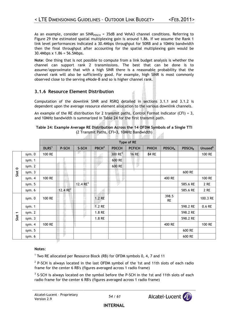
< LTE DIMENSIONING GUIDELINES – OUTDOOR LINK BUDGET> <FEB.2011>
Alcatel-Lucent – Proprietary
Version 2.9 54 / 61
INTERNAL
As an example, consider an SINRPDSCH = 35dB and VehA3 channel conditions. Referring to
Figure 29 the estimated spatial multiplexing gain is around 1.86. If we assume the Rank 1
link level performances indicated a 30.4Mbps throughput for 50RB and a 10MHz bandwidth
then the final throughput after accounting for the spatial multiplexing gain would be
30.4Mbps x 1.86 = 56.5Mbps.
Note: One thing that is not possible to compute from a link budget analysis is whether the
channel can support rank 2 transmissions. The best that can be done is to
assume/approximate that with a high SINR there is a reasonable probability that the
channel rank will also be sufficiently good. For example, high SINR is most commonly
observed close to the serving eNode-B and so is higher channel rank.
3.1.6 Resource Element Distribution
Computation of the downlink SINR and RSRQ detailed in sections 3.1.1 and 3.1.2 is
dependent upon the average resource element allocation to the various downlink channels.
An example of the RE distribution for 2 transmit paths, Control Format Indicator (CFI) = 3,
and 10MHz bandwidth is summarized in Table 24 for the first transmit path.
Table 24: Example Average RE Distribution Across the 14 OFDM Symbols of a Single TTI
(2 Transmit Paths, CFI=3, 10MHz Bandwidth)
Type of RE
DLRS1 P-SCH S-SCH PBCH4 PDCCH PCFICH PHICH PDSCHA PDSCHB Unused6
sym. 0 100 RE 0 RE 0 RE 0 RE 300 RE5 16 RE 84 RE 0 RE 0 RE 100 RE
sym. 1 0 RE 0 RE 0 RE 0 RE 600 RE 0 RE 0 RE 0 RE 0 RE 0 RE
sym. 2 0 RE 0 RE 0 RE 0 RE 600 RE 0 RE 0 RE 0 RE 0 RE 0 RE
sym. 3 0 RE 0 RE 0 RE 0 RE 0 RE 0 RE 0 RE 0 RE 600 RE 0 RE
sym. 4 100 RE 0 RE 0 RE 0 RE 0 RE 0 RE 0 RE 400 RE 0 RE 100 RE
sym. 5 0 RE 0 RE 12.4 RE3 0 RE 0 RE 0 RE 0 RE 0 RE 585.6 RE 2 RE
Slot 0
sym. 6 0 RE 12.4 RE2 0 RE 0 RE 0 RE 0 RE 0 RE 0 RE 585.6 RE 2 RE
sym. 0 100 RE 0 RE 0 RE 1.2 RE 0 RE 0 RE 0 RE 398.5
RE 0 RE 100.3 RE
sym. 1 0 RE 0 RE 0 RE 1.2 RE 0 RE 0 RE 0 RE 0 RE 598.2 RE 0.6 RE
sym. 2 0 RE 0 RE 0 RE 1.8 RE 0 RE 0 RE 0 RE 0 RE 598.2 RE 0 RE
sym. 3 0 RE 0 RE 0 RE 1.8 RE 0 RE 0 RE 0 RE 0 RE 598.2 RE 0 RE
sym. 4 100 RE 0 RE 0 RE 0 RE 0 RE 0 RE 0 RE 400 RE 0 RE 100 RE
sym. 5 0 RE 0 RE 0 RE 0 RE 0 RE 0 RE 0 RE 0 RE 600 RE 0 RE
Slot 1
sym. 6 0 RE 0 RE 0 RE 0 RE 0 RE 0 RE 0 RE 0 RE 600 RE 0 RE
Notes:
1 Two RE allocated per Resource Block (RB) for OFDM symbols 0, 4, 7 and 11
2 P-SCH is always located in the last OFDM symbol of the 1st and 11th slots of each radio
frame for the center 6 RB's (figures averaged across 1 radio frame)
3 S-SCH is always located on the symbol before the P-SCH in the 1st and 11th slots of each
radio frame for the center 6 RB's (figures averaged across 1 radio frame)
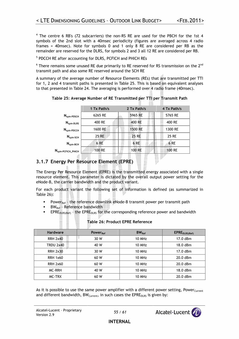
< LTE DIMENSIONING GUIDELINES – OUTDOOR LINK BUDGET> <FEB.2011>
Alcatel-Lucent – Proprietary
Version 2.9 55 / 61
INTERNAL
4 The centre 6 RB's (72 subcarriers) the non-RS RE are used for the PBCH for the 1st 4
symbols of the 2nd slot with a 40msec periodicity (figures are averaged across 4 radio
frames = 40msec). Note for symbols 0 and 1 only 8 RE are considered per RB as the
remainder are reserved for the DLRS, for symbols 2 and 3 all 12 RE are considered per RB.
5 PDCCH RE after accounting for DLRS, PCFICH and PHICH REs
6 There remains some unused RE due primarily to RE reserved for RS transmission on the 2nd
transmit path and also some RE reserved around the SCH RE
A summary of the average number of Resource Elements (REs) that are transmitted per TTI
for 1, 2 and 4 transmit paths is presented in Table 25. This is based on equivalent analyses
to that presented in Table 24. The averaging is performed over 4 radio frame (40msec).
Table 25: Average Number of RE Transmitted per TTI per Transmit Path
1 Tx Path/s 2 Tx Path/s 4 Tx Path/s
Nsym-PDSCH 6265 RE 5965 RE 5765 RE
Nsym-DLRS 400 RE 400 RE 400 RE
Nsym-PDCCH 1600 RE 1500 RE 1300 RE
Nsym-SCH 25 RE 25 RE 25 RE
Nsym-BCH 6 RE 6 RE 6 RE
Nsym-PCFICH_PHICH 100 RE 100 RE 100 RE
3.1.7 Energy Per Resource Element (EPRE)
The Energy Per Resource Element (EPRE) is the transmitted energy associated with a single
resource element. This parameter is dictated by the overall output power setting for the
eNode-B, the carrier bandwidth and the product variant.
For each product variant the following set of information is defined (as summarized in
Table 26):
� PowerRef – the reference downlink eNode-B transmit power per transmit path
� BWRef – Reference bandwidth
� EPREDLRS(Ref) – the EPREDLRS for the corresponding reference power and bandwidth
Table 26: Product EPRE Reference
Hardware PowerRef BWRef EPREDLRS(Ref)
RRH 2x40 30 W 10 MHz 17.0 dBm
TRDU 2x40 40 W 10 MHz 18.0 dBm
RRH 2x30 30 W 10 MHz 17.0 dBm
RRH 1x60 60 W 10 MHz 20.0 dBm
RRH 2x60 60 W 10 MHz 20.0 dBm
MC-RRH 40 W 10 MHz 18.0 dBm
MC-TRX 60 W 10 MHz 20.0 dBm
As it is possible to use the same power amplifier with a different power setting, PowerCurrent
and different bandwidth, BWCurrent, in such cases the EPREDLRS is given by:
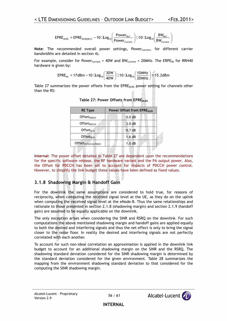
< LTE DIMENSIONING GUIDELINES – OUTDOOR LINK BUDGET> <FEB.2011>
Alcatel-Lucent – Proprietary
Version 2.9 56 / 61
INTERNAL
⋅+
⋅−=
Current
fRe10
Current
fRe10)f(ReDLRSDLRS
BW
BWLog10
Power
PowerLog10EPREEPRE
Note: The recommended overall power settings, PowerCurrent, for different carrier
bandwidths are detailed in section 4).
For example, consider for PowerCurrent = 40W and BWCurrent = 20MHz. The ERPERS for RRH40
hardware is given by:
dBm2.15MHz20
MHz10Log10
W40
W30Log10dBm17EPRE 1010RS =
⋅+
⋅−=
Table 27 summarizes the power offsets from the EPREDLRS power setting for channels other
than the RS:
Table 27: Power Offsets from EPREDLRS
RE Type Power Offset from EPREDLRS
OffsetPDSCH 0.0 dB
OffsetPDCCH 3.0 dB
OffsetSCH 0.7 dB
OffsetBCH 1.6 dB
OffsetPCFICH & PHICH 1.0 dB
Internal: The power offset detailed in Table 27 are dependent upon the recommendations
for the specific software release, the RF hardware variant and the PA output power. Also,
the Offset for PDCCH has been set to account for impacts of PDCCH power control.
However, to simplify the link budget these values have been defined as fixed values.
3.1.8 Shadowing Margin & Handoff Gain
For the downlink the same assumptions are considered to hold true, for reasons of
reciprocity, when computing the received signal level at the UE, as they do on the uplink
when computing the received signal level at the eNode-B. Thus the same relationships and
rationale to those presented in section 2.1.8 (shadowing margin) and section 2.1.9 (handoff
gain) are assumed to be equally applicable on the downlink.
The only exception arises when considering the SINR and RSRQ on the downlink. For such
computations the above mentioned shadowing margin and handoff gains are applied equally
to both the desired and interfering signals and thus the net effect is only to bring the signal
closer to the noise floor. In reality the desired and interfering signals are not perfectly
correlated with each another.
To account for such non-ideal correlation an approximation is applied in the downlink link
budget to account for an additional shadowing margin on the SINR and the RSRQ. The
shadowing standard deviation considered for the SINR shadowing margin is determined by
the standard deviation considered for the given environment. Table 28 summarizes the
mapping from the environment shadowing standard deviation to that considered for the
computing the SINR shadowing margin.

< LTE DIMENSIONING GUIDELINES – OUTDOOR LINK BUDGET> <FEB.2011>
Alcatel-Lucent – Proprietary
Version 2.9 57 / 61
INTERNAL
Table 28: Mapping from Environment Shadowing Standard Deviation to the Shadowing
Standard Deviation Used for Computing SINR Shadowing Margin
Environment
Shadowing Std. Dev.
DL SINR
Shadowing Std.
Dev.
6 dB 0 dB
7 dB 1 dB
8 dB 2 dB
The same method as detailed in section 2.1.8 is used to compute the SINR shadowing
margin based on the SINR shadowing standard deviations presented in Table 28.
Note: Close agreement has been observed when comparing field measured SINR and RSRQ
distributions with predicted SINR and RSRQ distributions that account for a shadowing
margin based on the standard deviations presented in Table 28.
3.2 Downlink Budget Example
Table 29 presents some example of the entire downlink budget analysis for a dense urban
environment with deep indoor penetration for a range of different services. Note that this
is the downlink link budget that corresponds to the uplink budget presented in Table 20.
The key objective of the downlink link budget analysis is to formulate estimates of the
data rate expectations for the cell ranges of some nominal uplink data rates (see the
rows in red in Table 29).

< LTE DIMENSIONING GUIDELINES – OUTDOOR LINK BUDGET> <FEB.2011>
Alcatel-Lucent – Proprietary
Version 2.9 58 / 61
INTERNAL
Table 29: Typical PDSCH link budgets for a RRH deployment in Dense Urban VehA3
channel conditions at 700MHz (uplink 128kbps guaranteed at cell edge)
It is important to note that the downlink data rate estimates presented in the last row of
Table 29 are achievable with 95% coverage reliability over the downlink cell ranges
indicated in the row titled “UL Service Cell Range”. Note also that the same data rates are
achieved over the entire coverage area (1.24km cell range) with reduced reliabilities for
the higher data rates.
Internal: The default ALU link budget can be found on the intranet: Alcatel-Lucent LTE-
FDD & TDD Link Budget.

< LTE DIMENSIONING GUIDELINES – OUTDOOR LINK BUDGET> <FEB.2011>
Alcatel-Lucent – Proprietary
Version 2.9 59 / 61
INTERNAL
4 DOWNLINK OUTPUT POWER
Assuming that the carrier bandwidth is known it is important to size the downlink power
amplifier to ensure sufficient DL power resources to match the targeted uplink coverage.
A series of system simulation studies were performed to assess the required Power
Amplifier (PA) sizing for 4 different cases
� 700 MHz (10 MHz)
� 2.1 GHz (10 MHz)
� 2.1 GHz/AWS (5 MHz)
� 2.6 GHz (20 MHz)
All scenarios considered 2x2 MIMO on the DL and 2RxDiv on the UL.
In principle, all of the studies concluded that spectrum efficiency for “reasonable” cell
sizes is relatively invariant to reasonable choices of PA sizes and that edge rates become
much more sensitive to the choice of power at large cell radiuses.
The process for assessing the downlink power requirements is summarized below:
� Step 1: Confirm uplink edge data rate MAPL, i.e. 64 kb/s or higher through the use
of link budget
� Step 2: Determine the cell range based on the link budget for 64kb/s or other rate
� Step 3a: Run downlink system simulations using same cell size/range & other link
budget requirements (use CDMA power levels for guidance) and variable PA Size to
confirm that edge data rate requirements for the downlink are met
� Step 3b: Alternatively construct a downlink link budget (variations in loading &
interference, benefit of multi-user scheduling, frequency selective scheduling,
HARQ, can not be well modeled in downlink link budgets) and confirm that edge
data rate requirement can be met
� Step 4: Perform uplink system simulations and observe cell edge rate meets link
budget requirements
Table 30 summarizes the recommended PA sizing based on the observations from the above
mentioned study (independent of the frequency band).
Table 30: Recommended Power Amplifier Sizing
Carrier Bandwidths PA Power
1.4 MHz 2 x 20 W
3.0 MHz 2 x 20 W
5.0 MHz 2 x 20 W
10.0 MHz 2 x 30 W
15.0 MHz 2x40 W
20.0 MHz 2 x 40 W

< LTE DIMENSIONING GUIDELINES – OUTDOOR LINK BUDGET> <FEB.2011>
Alcatel-Lucent – Proprietary
Version 2.9 60 / 61
INTERNAL
5 RADIO NETWORK PLANNING
The key motivations for utilizing an RNP tool for LTE design purposes include:
� Enhancement of the accuracy of the initial link budget design by accounting for
field constraints such as the topology, morphology and traffic distribution. Site
positions, antenna heights, antenna tilts can also be optimized.
� Accounting more accurately for the interference (geometry) scenario encountered
for the specific deployment
It is the later point that is particularly important for LTE downlink coverage considerations.
The approach recommended by Alcatel-Lucent is to formulate an UL link budget to define
the cell range and then within that cell range perform an RNP study on the DL to assess the
SINR performances achievable at the cell edge. This allows the following points to be
assessed:
� Whether the DL is interference or noise limited
o If noise limited, a higher output power configuration should be considered
� Whether the corresponding DL cell edge performances satisfy the DL cell edge
performance expectations
o This will drive the required bandwidth, output power and MIMO
configuration on the DL
Alcatel-Lucent relies on the 9955 RNP tool, based on the ATOLL platform developed by
FORSK. 9955 is fully aligned with Alcatel-Lucent’s products and engineering tool chain.
Alcatel-Lucent customers can fully benefit from this tool since it is included in Alcatel-
Lucent’s product portfolio.

< LTE DIMENSIONING GUIDELINES – OUTDOOR LINK BUDGET> <FEB.2011>
Alcatel-Lucent – Proprietary
Version 2.9 61 / 61
INTERNAL
6 SUMMARY
This document has introduced the detailed formulation of Alcatel-Lucent’s LTE FDD link
budget for outdoor macro cellular deployments for both the uplink and the downlink.
LTE coverage is not considered to be limited by the downlink for typical eNode-B output
powers and deployment scenarios. Link budgets should remain uplink limited and as such
link budgets are used by Alcatel-Lucent primarily to derive the expected LTE performances
at the cell edge on the uplink and compare them with legacy systems in the case of an
overlay of an existing network and/or the required number of sites for a Greenfield
operator. In the case of overlay deployments, this allows for the estimation of the
proportion of sites that can be reused (additional constraints such as space for hardware
deployment, etc, have to be considered on top of this).
The downlink link budgets that have been detailed here are indicative of what rates are
achievable within the corresponding uplink service coverage areas. It is important to
understand that downlink cell edge performances are strongly dependent upon scheduler
parameters (e.g. tuning of the fairness of the proportional fair scheduler algorithm) or the
available bandwidth (e.g. 10MHz vs 5MHz)
Downlink performances in the link budget are based only on long term average PDSCH SINR
values and do not account for dynamic channel variations that can be addressed with
frequency selective scheduling functionalities
Better estimates of downlink performances can be achieved by means of system level
simulations and/or Radio Network Planning (RNP) analysis.
END END END END OF DOCUMENTOF DOCUMENTOF DOCUMENTOF DOCUMENT