01/05/2012 presentation: stress-based fatigue monitoring

Tim Gilman Associate NRC Fatigue Meeting January 5, 2012

Stress-Based Fatigue Monitoring: Methodology for Fatigue Monitoring of Class 1 Nuclear Components in a Reactor Water Environment (EPRI technical report 1022876)

2 © 2011 Electric Power Research Institute, Inc. All rights reserved.

Presentation Objective

• Present EPRI-sponsored methodology for stress-based environmental fatigue monitoring which addresses RIS 2008-30. • Obtain concurrence from NRC that general approach

outlined here resolves the concerns expressed in the RIS.


General Objectives of EPRI Report

• Resolve regulatory concerns about use of single stress term in fatigue monitoring (RIS 2008-30). • Provide for automatic calculation of environmentally-

assisted fatigue (EAF) – not just ASME Code fatigue.


NRC Position on Fatigue

• Draft NRC RIS-2008-XX (“Fatigue Analysis of Nuclear Power Plant Components” May 2008) was issued to inform licensees of NRC staff concern about use of simplified single stress term in fatigue evaluations. • NRC responded to public comments on the draft RIS in

Dec 2008. • Final RIS-2008-30 issued Dec 2008. • Fatigue calculations must consider all six stress

components in accordance with ASME Subarticle NB-3200 guidance.


What is Stress-Based Fatigue (SBF)?

• Actual plan measured data (temperatures, pressures, flow rates, valve positions, etc.) are used to compute detailed stress histories.

• From the stress histories, fatigue usage factors are computed for monitoring purposes.


FatiguePro and RIS-2008-30

• Historically, single stress term sometimes used for fatigue evaluations – Originally necessary because of computer limitations – Conventional stress cycle counting algorithms use

single stress – Simplified methodology can be shown to be

conservative, but great deal of judgment may be required for development

• Subsequent RAIs related to fatigue analysis question analyst judgments involved in general.


Guiding Principles for Development

• Accuracy – Benchmarks reproduce known problems – Meet design basis (ASME Subarticle NB-3200) and

regulatory requirements (NUREG-1801, GALL Report) – Industry guidance (EPRI’s EAF Expert Panel lessons)

• Validation – Results make physical sense. – Consistent with sound science and engineering principles.

• Repeatability – Comply with ASME NQA-1 – Minimize analyst and user judgments

• Transparency – Technical basis documented in EPRI report – Available for everyone to review


SBF Technical Basis Significant Areas of New Technology

• Stress calculations (linearized membrane, bending, and peak components) • Stress peak and valley detection • Stress cycle pairing and fatigue calculations • Environmental fatigue (Fen) calculations


Stress Calculation Objectives

• Compute time history of the 6 unique stress components for: – Primary plus secondary (usually

linearized membrane plus bending) – Total stresses (including peak)

• Plus metal surface temperature

Time SX SY SZ SXY SYZ SXZ SX SY SZ SXY SYZ SXZ Temp0 2.281 47.413 37.257 1.772 0.000 0.000 0.128 72.722 63.606 0.097 0.000 0.000 154.31 2.291 47.830 37.637 1.762 0.000 0.000 0.130 73.226 64.094 0.096 0.000 0.000 149.42 2.301 48.245 38.014 1.752 0.000 0.000 0.131 73.726 64.579 0.095 0.000 0.000 144.63 2.313 48.607 38.301 1.755 0.000 0.000 0.132 74.181 64.973 0.095 0.000 0.000 142.84 2.323 48.972 38.598 1.756 0.000 0.000 0.134 74.638 65.376 0.094 0.000 0.000 140.55 2.333 49.357 38.939 1.749 0.000 0.000 0.135 75.053 65.767 0.093 0.000 0.000 136.6

Primary (P) + Secondary (Q) Primary (P) + Secondary (Q) + Peak (F)


Stress Calculations (cont’d)

• Linearized stresses for static loads are scalable – Pressure – Piping interface loads (forces, moments)

• Thermal (time-dependent) stresses are calculated with Green’s Functions – Green’s Functions are simply influence functions – The RIS clearly states, “The Green’s function

methodology is not in question.”


Linearized Thermal Stresses

• Requires use of appropriately conservative ratio of (P+Q) to (P+Q+F) (analyst judgment or previously performed fatigue analysis), OR • Accurate knowledge of time-dependent, through-wall stress distribution

Implemented the latter to improve accuracy and minimize analyst judgments.


Linearized Thermal Stresses (cont’d)

• Use of either Lagrange Polynomial: • or piece-wise linear distribution

pp xHxHxHHy ++++= 2

210

-300000

-250000

-200000

-150000

-100000

-50000

0

50000

0 0.5 1 1.5 2 2.5

Hoo

p St

ress

(psi

)

Distance x (inches)

SZ (Lagrange Fit)

SZ (ANSYS)

Piece-Wise Linear



• Conventional membrane and bending stress computations. – “Cartesian” or generalized linearization in ANSYS – “Linearization for three-dimensional structures” in ABAQUS – Stress Linearization Procedure described in Section

5.A.4.1.2 of ANNEX 5.A of ASME Section VIII, Division 2

dxxtxt

dxxt

t

b

t

m

∫

∫

−=

=

02

0

2)(6

)(1

σσ

σσ Closed form solutions using previously determined Lagrange Polynomial



-60000

-40000

-20000

0

20000

40000

60000

80000

100000

120000

0 0.1 0.2 0.3 0.4 0.5 0.6 0.7 0.8

Stre

ss (p

si)

Distance x (inches)

TOT (Lagrange)

M+B (Lagrange)

M (Lagrange)

TOT (Piece-Wise Linear)

M+B (Piece-Wise Linear)

M (Piece-Wise Linear)


Multiaxial Green’s Function

Macro developed to create multiaxial Green’s Function. Includes all information necessary to compute linearized thermal stresses at a stress classification line for a given film coefficient.


Computation of Primary Plus Secondary and Total Stresses

• Pressure, piping interface, and other “static” loads added together by scaling to pressure, temperature, etc. – M+B and Total

• Through-wall time-dependent thermal stresses computed using Green’s Functions – All six M+B components computed based on through-

wall distributions • Fatigue strength reduction factors applied on M+B

stresses, as appropriate • Thermal peak is superimposed after the FSRF/SCF is

applied. • Same methodology implemented as in the EPRI EAF

Expert Panel sample problem.


Benchmark of Stress Calculations

• Sample problem from EPRI’s EAF Expert Panel performed • Comparisons made to values computed with ANSYS

using temperature-dependent material properties. – Total stress – Membrane plus bending stress – Temperature


-200

-150

-100

-50

0

50

100

150

200

0 500 1000 1500 2000 2500 3000 3500

SX_p

SY_p

SZ_p

SXY_p

SX_p_FP

SY_p_FP

SZ_p_FP

SXY_p_FP

Benchmark of Total Stresses

Total Stresses


-80

-60

-40

-20

0

20

40

60

80

0 500 1000 1500 2000 2500 3000 3500

SX_n

SY_n

SZ_n

SXY_n

SX_n_FP

SY_n_FP

SZ_n_FP

SXY_n_FP

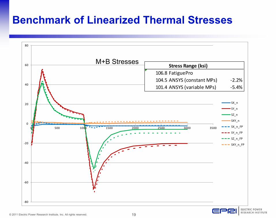
Benchmark of Linearized Thermal Stresses

M+B Stresses Stress Range (ksi)

106.8 FatiguePro104.5 ANSYS (constant MPs) -2.2%101.4 ANSYS (variable MPs) -5.4%


Benchmark of Metal Temperature Calculations

0

100

200

300

400

500

600

700

0 500 1000 1500 2000 2500 3000 3500

Tm_ANSYS (constant MPs) Tm_FatiguePro Tm_ANSYS (variable MPs)


Stress Cycle Counting Design vs. Monitoring

• Design Assumptions – Idealized transient definitions – Maximum number of cycles – Cycles postulated to occur in worst-possible order

• Monitoring – Real data – Typically less severe stress ranges, but increased

complexity – Cycles are known to occur in actual order

Taking order into account using all six stress components and other ASME Code rules requires a non-trivial solution!


Idealized ASME “Stress Cycle”

“… a condition where the alternating stress difference [NB-3222.4(e)] goes from an initial value through an algebraic maximum value and an algebraic minimum value and then returns to the initial value.”

An “operational cycle” can contain multiple stress cycles.

2∙Salt


Stress Cycles Traditional Design Analysis Example

Transient order unknown Local extreme stress conditions (peaks or valleys) assumed to pair in worst-possible order.


Stress Cycles Monitoring Example

• Local extreme conditions evaluated in known order.

• One large stress reversal with multiple internal cycles.

• Factor of 10 (possibly more, depending on analyst judgment) difference using known order.

-100

-50

0

50

100

150

200

Stre

ss (k

si)

Stress History

Sp Ke Salt n Nallow U200 3.333 333.3 1 54.47 0.01835873

50 1 25 18 1481072 1.21534E-05CUF = 0.018


Stress Cycle Monitoring Example

-40

-35

-30

-25

-20

-15

-10

-5

0

5

10

0 500 1000 1500 2000 2500St

ress

(ksi

)

Fact: Fatigue is path (order) dependent!

One stress cycle

Below endurance limit


Counting Ordered Stress Cycles Using Single Stress Term

• Fatigue damage under random loading studied extensively in auto and aerospace industries. • Several methods are available:

– Range-pair – Rainflow – Ordered Overall Range (OOR)

• These different numerical methods produce essentially the same results. • These methods are generally limited to single stress term

using conventional algorithms.


Rainflow Algorithm

• Simplified Rainflow Cycle Counting Method documented in ASTM Standard No. E1049 (Reapproved 2005). Standard practices for cycle counting in fatigue analysis. • ASME Section VIII Division 2 Annex 5.B (non-mandatory

guidance). • Peaks imagined as source of water that "drips" down a

pagoda roof. • Conventional algorithm uses single stress term • Proportional loading


Order Dependence in ASME Code

ASME Code does not prohibit consideration of order. Methods for handling seismic events reflect order dependence. Transient pair stress range increased by OBE stress amplitude. Remainder are internal (self) cycles.

Internal OBE cycles

Transient stress range without OBE

New transient stress range increased by OBE stress amplitude


The Multiaxial Challenge

• NB-3216.2 provides guidance in computing stress intensity difference when normal and shear stresses may vary arbitrarily, and the “stress cube” that determines principal stresses may rotate. • Challenge: SI between two points in a cycle is not equal to

the stress intensity difference, which is determined based on the difference of the 6 individual stress components in going from one cycle to another.

How to account for ordered stresses while meeting requirements and intent of ASME Code?

“In most cases it will be possible to choose at least one time during the cycle when the conditions are known to be extreme. In some cases it may be necessary to try different points in time to find the one which results in the largest value of alternating stress intensity.”


Example - Charging Nozzle

• High steady state thermal gradient during cold injection. • Difficulty with “design”

type stress cycle pairing illustrated with complexity of real data.


Charging Nozzle – Plant Heatup

0

100

200

300

400

500

600

-10000

0

10000

20000

30000

40000

50000

60000

Tem

pera

ture

(F)

Stre

ss (p

si)

SX

SY

SZ

SXY

SYZ

SXZ

TCHG

Tm

TCOLD

DESIGN_TCHG

Real data is much more complex than design transients. What do we need to consider? What can we ignore?


Solution Alternatives

• A solution to the problem requires two important steps. – Multiaxial peak and valley detection logic – Multiaxial stress cycle pairing logic

• Several options investigated for each. • Used together, “Rubberband” and “Rainflow-3D”

produced best results across many test cases.


Criteria for Selection of Algorithm How do we know what’s right?

• When simulated in the same order, we should reproduce known problems from ASME NB-3200 design calculation examples (benchmarks for accuracy) • Assuming a uniaxial stress with random, ordered loading,

we should with our algorithms identify the same stress cycles as that from heavily vetted algorithms such as Rainflow (validation of sound engineering principles) • Analyst judgments and manual adjustments to the stress

cycle counting should not be necessary to produce consistently meaningful results (repeatability of results)


Peak/Valley Detection – “Rubberband”

• Detects points of maximum distance from the previous possible extrema.

• Looks for SI range to increase from previous extrema to a given threshold and then decrease to another threshold to identify a new extrema.

• Range varies in multiple dimensions.

• Filters out insignificant reversals well below the endurance limit

• Range of time included for each


Peak/Valley Detection – “Rubberband”

0

100

200

300

400

500

600

700

-200

-150

-100

-50

0

50

100

150

0 500 1000 1500 2000 2500 3000 3500

Tem

pera

ture

( °F)

Stre

ss (k

si)

SX_n

SY_n

SZ_n

SXY_n

SX_p

SY_p

SZ_p

SXY_p

Temp, °F

Peak

Valley

PVs are time windows to ensure conservative stress range computations.


“Rubberband” Addresses General Concern in NRC RIS 2011–14 (December 29, 2011)

• By taking order and multiaxial stress range into account, manual peak and valley adjustment is not required. • Process is predictable, repeatable and conservative.

“Although this method of analyst intervention [manual modification of peaks and valleys] could provide acceptable results in some cases, reliance on the user’s engineering judgment and ability to modify peak and valley times/stresses, without control and documentation, could produce results that are not predictable, repeatable, or conservative.”


Pairing Logic – “Rainflow-3D”

• Conventional Rainflow algorithm implemented, but with following differences – SI range is computed between local extrema based on

all six components of stress (instead of the algebraic difference in two values)

– Each extrema contains at least one time point and likely represents a time window of more than one point.

– Most conservative range pair selected based on combination of stress range, Ke (function of primary plus secondary stress intensity range) and the elastic modulus ratio.


Example – EAF Sample Problem Transient 1 – SCL 1

001i

001j-150

-100

-50

0

50

100

0 500 1000 1500 2000 2500 3000

Stress

[ksi]

Time [sec]

Sx Sy Sz Sxy Syz Sxz

Peak and valley “time windows” in red. Fatigue pair points marked with triangles.

All pertinent fatigue parameters reproduced! ____SR___ ____Sn___ __Ke__ ____Sa___ ____Na___ ____Ui___ 280.6228 118.2572 3.333 518.9791 29.17570 0.034275 --------- --------- ------ --------- --------- ---------


Operational Cycle with Multiple Stress Cycles

001i

001j

002i

002j003j

004i

004j

-125

-100

-75

-50

-25

0

25

50

75

0 500 1000 1500 2000 2500 3000 3500

Stress

[ksi]

Time [sec]


____SR___ ____Sn___ __Ke__ ____Sa___ ____Na___ ____Ui___ 43.12391 16.56381 1.000 23.10216 268848.4 3.720e-06 80.63670 28.46853 1.000 44.45877 18579.07 5.382e-05 27.36576 10.77131 1.000 14.34155 1.560e+07 6.409e-08 204.7023 82.87598 3.119 357.1089 63.14125 0.015838 --------- --------- ------ --------- --------- --------- CUF = 0.015895

Pairing with end state demonstrates order dependence!


Charging Nozzle – Simulated Loss of Letdown with Delayed Return to Service

001j002i

002j

-25

0

25

50

75

100

125

0 100 200 300 400 500 600 700 800 900 1000 1100 1200

Stress

[ksi]

Time [sec]


This example uses two Green’s Functions and superposition of stresses – 1 for charging flow surface and one for the reactor coolant flow surface.


Charging Nozzle – Multiple Letdown Trips

001i

001j

002i

002j

-10

0

10

20

30

40

50

60

70

80

90

100

110

120

46000 47000 48000 49000 50000 51000 52000 53000 54000 55000

Stress

[ksi]

Time [sec]



Environmentally-Assisted Fatigue

• Methodology takes guidance from EPRI’s EAF Expert Panel recommendations. • Panel has reached general consensus on computation of

strain rate using multiaxial stresses. • Generally consistent with proposed Code case on strain

rate (ASME Record No. 10-293) – ASME Code Case N-792-1


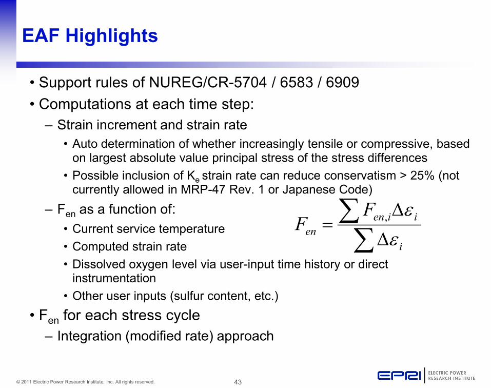
EAF Highlights

• Support rules of NUREG/CR-5704 / 6583 / 6909 • Computations at each time step:

– Strain increment and strain rate • Auto determination of whether increasingly tensile or compressive, based

on largest absolute value principal stress of the stress differences • Possible inclusion of Ke strain rate can reduce conservatism > 25% (not

currently allowed in MRP-47 Rev. 1 or Japanese Code)

– Fen as a function of: • Current service temperature • Computed strain rate • Dissolved oxygen level via user-input time history or direct

instrumentation • Other user inputs (sulfur content, etc.)

• Fen for each stress cycle – Integration (modified rate) approach

∑∑

∆∆

=i

iienen

FF

εε,


EAF Sample Problem Calculation



0

0.001

0.002

0.003

0.004

0.005

0.006

0.007

0.008

0.009

0.01

-200

-150

-100

-50

0

50

100

150

0 500 1000 1500 2000 2500 3000 3500

SY Fen∙de


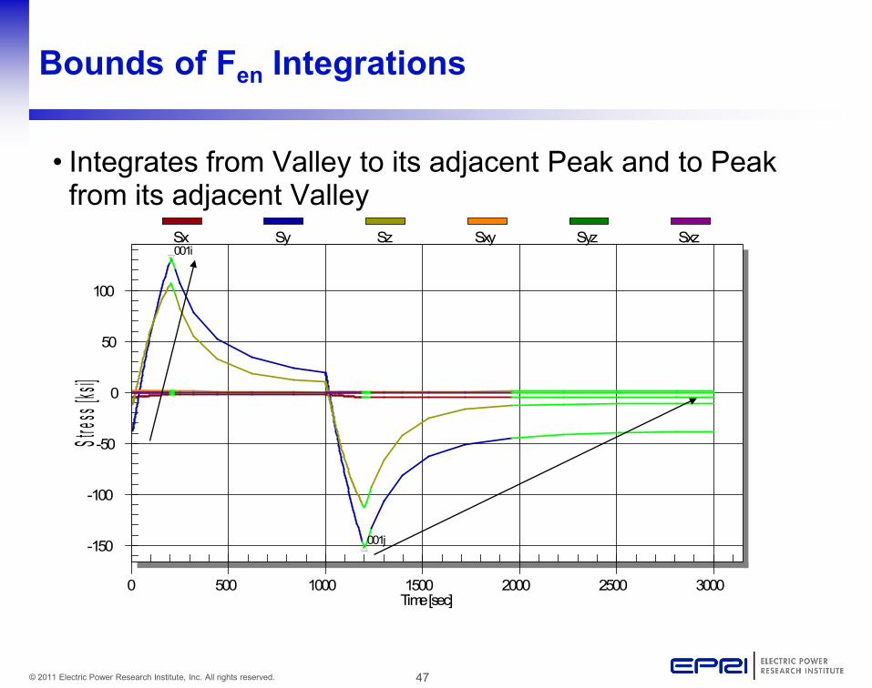
Bounds of Fen Integrations

• Integrates from Valley to its adjacent Peak and to Peak from its adjacent Valley

001i

001j-150

-100

-50

0

50

100

0 500 1000 1500 2000 2500 3000

Stress

[ksi]

Time [sec]



Fen’s for Complex Stress Cycling

001i

001j

002i

002j003j

004i

004j

-125

-100

-75

-50

-25

0

25

50

75

0 500 1000 1500 2000 2500 3000 3500

Stress

[ksi]

Time [sec]



Conclusions

• Overall methodology combines many proven practices • Basic steps in the process include:

– Multiaxial stress calculations • Address NRC RIS 2008-30 • Accurate knowledge of through-wall distributions

– Smart Peak/Valley Detection and Stress Cycle Counting • Rubberband (detects reversal regions using multiaxial

stress range criteria) • Rainflow-3D (identifies stress cycles)

– Calculation of EAF • Meets GALL requirements • Implements Expert Panel guidance


Questions and Comments

01/05/2012 presentation: stress-based fatigue monitoring

Documents