Motion Estimation for MovingTarget Detection

VISHAL MARKANDEY, Member, IEEE

ANTHONY REID, Member, IEEE

SHENQ WANG, Member, IEEETexas Instruments

This paper describes a suite of techniques for the autonomous

detection of moving targets by processing electro-optical sensor

imagery (such as visible or infrared imagery). Specific application

scenarios that require moving target detection capability are

described, and solutions are developed under the constraints

imposed by the scenarios. Performance evaluation results are

presented using a test data set of over 300 images, consisting

of real imagery (visible and infrared) representative of the

application scenarios.

Manuscript received November 16, 1992; revised December 15, 1995.

IEEE Log No. T-AES/32/3/05861.

Authors’ addresses: V. Markandey, Digital Video Products, TexasInstruments, Dallas, TX 75265; A. Reid and S. Wang, SystemsTechnology Center, Systems Group, Texas Instruments, Plano, TX75086.

0018-9251/96/$10.00 c° 1996 IEEE

I. INTRODUCTION

The autonomous detection of moving targets usingelectro-optical sensor imagery is a requirement inseveral defense application scenarios. Examples ofsuch applications are: detection of moving targetsfrom a surveillance post, a missile flyby search forground-based moving targets, and the detection ofairborne targets from an airborne platform. Eachapplication imposes a unique set of constraints, andthe solution developed needs to take these constraintsinto account. For example, the detection of movingtargets from a stationary platform can be addressed bydetecting the presence of motion in an image sequenceand compensating for sensor drift if necessary. Onthe other hand, in applications that involve significantsensor motion, motion detection alone is not enough.Sensor motion creates apparent background motionin the imagery, and this motion can be significantlygreater than the target motion. Compensation forapparent background motion by image registration andsegmentation of motion information into target andbackground motion is required in such a scenario.The first step in the detection of moving targets

in image sequences is the detection and estimationof motion from sensor data. The detection of motioncan be performed by simple operations such as imagedifferencing followed by thresholding, and is thusattractive from a computational standpoint. Howeverits applicability is limited to scenarios where thereis no background motion. Motion estimation canprovide a richer source of information that can beuseful not only in target detection but also in thefollow-on activity of target tracking. Motion estimationtechniques that provide motion measurement (opticalflow) at every pixel location in the image planeare particularly attractive as they can be useful inthe detection of low contrast targets. While suchtechniques have been extensively developed andstudied in the fields of computer vision and imageprocessing, not much has been done in applyingthem to moving target detection. We have appliedmotion estimation and analysis techniques to variousapplication scenarios within the domain of movingtarget detection. Each scenario imposes its own uniqueconstraints on the problem and the solution has totake these constraints into account. This has led usto develop several new results in motion estimationand analysis–primary among them being robustmotion estimation in the presence of noise, andmultiresolution motion estimation for moving sensorscenarios. We have also developed new techniquesto process the motion estimates to produce usablemeasures of target detection. In this work we describeour development of motion estimation techniques,their application to moving target detection applicationscenarios, and the results of testing on real imagery.Please note that we do not address target tracking

866 IEEE TRANSACTIONS ON AEROSPACE AND ELECTRONIC SYSTEMS VOL. 32, NO. 3 JULY 1996

here. Our focus is on moving target detection. Thedetection results can certainly be useful in tracking (assay in initializing a tracker), but in this work we limitourselves to the detection problem alone.The rest of this work is organized as follows. In

the rest of this section we describe the techniquesavailable in literature for both motion estimation andmoving target detection. In Section II we describemotion estimation techniques that we have developedfor several moving target detection applicationscenarios. In Section III we describe motion analysistechniques that analyze the motion estimates providedby Section II, to achieve moving target detectionfunctionality. In Section IV we provide results ofexperimental testing of our techniques.One of the common approaches to pixel level

motion estimation or optical flow computation, isbased on the brightness constancy assumption [5],which states that if I(x,y, t) is the image intensity atpixel (x,y) at time t then:

dI

dt= 0: (1)

Application of the chain rule to the term on theleft-hand side gives

Ixu+ Iyv+ It = 0: (2)

Here Ix, Iy, and It are the partial derivatives of Iwith respect to x, y, and t, respectively, and (u,v)are the optical flow components. Horn and Schunck[5] proposed an iterative technique for computingoptical flow. They solved (2) for (u,v) by imposinga smoothness requirement on the flow field andminimizing an error functional in terms of accuracyand smoothness. A drawback of this technique fromthe moving target detection standpoint is that itsmooths across motion boundaries of objects, smearingmotion discontinuities caused by occluding contours.Other techniques have developed solutions to (2)

for (u,v) by alternate additional constraints. Wohn,et al. [14] applied constancy assumptions to imagefunctions such as spatial gradient magnitude, curvature,and moments. In similar work, constraints for solving(2) were obtained by applying constancy assumptionsto image functions such as contrast, and entropy in[9]. Schunck [11] developed a technique that solves (2)after transforming it into a polar form. This form isconsidered convenient for representing image flowswith discontinuities, as the polar equation will not have±-functions at discontinuities. Koch, et al. [7] addressedthe problem of smoothing across discontinuities byusing the concept of binary line processes whichexplicitly mark the presence of discontinuities. Theline process terms are encoded as a modification ofthe Horn and Schunck [5] minimization terms forsmoothness.While (1) has been used as the basis of many

optical flow techniques as discussed above, it is not

a realistic assumption in many cases. It requires thatthe image brightness corresponding to a physicalsurface patch remain unchanged over time. This isnot true when points on an object are obscured orrevealed in successive image frames, or when an objectmoves such that the light is incident at a given pointon the object from a different angle. This causes thesurface shading to vary. In view of this, Corneliusand Kanade [2] developed a variation fo the Hornand Schunck method. In their formulation (1) neednot hold true, and gradual changes are allowed in theway an object appears in a sequence of images. Thisis done by defining a smoothness measure for changein brightness variation and an error measure between(1) and (2), and minimizing a weighted sum of thesetwo quantities and the spatial gradient of the velocitycomponents defined by Horn and Schunck. Gennertand Negahdaripour [3] expanded further on this idea.Their approach allows a global linear transformationbetween brightness values in consecutive images. Theapproaches of Cornelius and Kanade, and of Hornand Schunck, can be shown to be special cases of thismethod. They provide qualitative results to show thattheir technique performs better than the Horn andSchunck, and Cornelius and Kanade techniques undercertain changing illumination conditions.Instead of considering the brightness constancy

assumption (1) as the starting point of optical flowcomputation, a gradient constancy requirement wasused in [4, 12]. This gradient constancy assumption isembodied by the equation,

d

dtrI = 0 (3)

where r is the spatial gradient operator over the imageplane. Equation (3) can be rewritten as

Ixxu+ Ixyv+ Ixt = 0 (4)

Ixyu+ Iyyv+ Iyt = 0 (5)

where (u,v) are the optical flow components. Opticalflow computation algorithms based on the gradientconstancy assumption require the solution of twolinear equations to compute the optical flow, acomputationally simple noniterative operation. Bycontrast the brightness constancy based algorithms aremuch more computationally complex (e.g., some ofthem are iterative). Thus gradient constancy algorithmshave a computational advantage over brightnessconstancy algorithms. On the other hand, gradientconstancy algorithms tend to be more noise sensitivethan brightness constancy algorithms because theyuse second-order image derivatives while brightnessconstancy algorithms use firt-order image derivatives.The motion estimation techniques discussed

so far are relevant to target detection from astationary sensor or where the apparent backgroundmotion in the imagery (induced by sensor motion)

MARKANDEY ET AL.: MOTION ESTIMATION FOR MOVING TARGET DETECTION 867

is of comparable magnitude to the target motionas perceived in the imagery. However there areapplication scenarios such as air-to-ground targetdetection or air-to-air target detection, where thecamera-induced sensor motion is often significantlygreater than the targets of interest. This means that inorder to achieve moving target detection functionality,image analysis must be precise enough to detect thesmall differential in the apparent motions of target andbackground in the image plane. Also, camera-inducedscene motion can be nonuniform across the image,due to perspective effects and sensor maneuvering. Anexample is closure, where the apparent backgroundmotion due to sensor motion is zero at the focus ofexpansion and has varying magnitude and direction indifferent parts of the image. Motion estimation andanalysis techniques should be able to distinguish sucheffects from the effects of target motion in imagery.The simple optical flow computation techniquesdiscussed above prove inadequate in such cases, andmore sophisticated techniques are needed for thecomputation of optical flow fields accurate enough torepresent the subtle variations due to target motion.A technique developed by Burt, et al. [1] computes

estimates of motion at various scales, or levels ofimage resolution, for the moving sensor movingtarget detection problem. Initial motion estimatescomputed at low resolution are used to registerimagery at successive levels of resolution and residualmotion estimates are computed at each resolutionlevel. Registration continues until the background iscompletely registered and the only apparent motion ina sequence is due to target motion. Image differencingis then used to discern the moving target regions.A shortcoming of this method is that, dependingon the differential between magnitudes of targetand apparent background motion, unless one knowsa priori when to stop the registration process, onecould register the target as well as background, sothat the moving targets are not detected in the finaldifference imagery. Also, the technique may notwork when the magnitudes of target and apparentbackground motion are similar (e.g., some cases ofpanning sensors), or if part of the apparent backgroundmotion is smaller in magnitude than target motion(e.g., in case of closure).The preceding discussion focused on the estimation

of motion, the first step of moving target detection.The motion estimates have to be further processed toproduce the final output of moving target detection:a target list containing centroid and bounding boxinformation of detected targets. For stationary sensors(including sensors with drift), optical flow discontinuitydetection and histogram segmentation approacheshave been used by Russo, et al. [10] to demonstratethe feasibility of performing moving target detection.These techniques provide only a visual output, and notan explicit target list.

II. MOTION ESTIMATION FOR MOVING TARGETDETECTION

All of the techniques described in Section I forbrightness constancy and gradient constancy basedoptical flow computation have one shortcoming incommon: they do not take into account the fact thatin real applications, noise is invariably present inthe image intensity measurements and will lead toviolations of their constancy assumptions. Opticalflow fields computed from these techniques using real,noisy data can therefore be noise sensitive. Attemptsare usually made in these techniques to reduce noiseeffects by performing spatial smoothing operations onthe flow field estimates computed from the constraints.Such attempts have limited applicability because oftheir ad hoc nature.The least squares technique proposed by Kearney

[6] differs from the approaches enumerated above, inthat it provides a formal, mathematical mechanismto account for the presence of noise in imagemeasurements. This technique is based on theassumption that the optical flow field is constantwithin a spatial neighborhood of a pixel. A brightnessconstancy constraint (2) is obtained from each pixelin this neighborhood, leading to an overconstrainedsystem of linear equations of the optical flowcomponents, i.e.,2666664

Ix1 Iy1

Ix2 Iy2

......

Ixn Iyn

3777775·u

v

¸=¡

266664It1

It2...

Itn

377775 (6)

where 1,2, : : : ,n are pixel indices. This is a linearsystem of equations of the general form

A~x= ~b (7)

where A and ~b are the measurements and ~x isthe parameter being estimated. The least squarestechnique assumes that noise is present only in ~b (as±~b), and minimizes the cost function

²LS = k±~bk2F = kA~x¡~bk2F (8)

where k ¢ kF is the Frobenius norm, defined for anM £N matrix C as

kCkF =vuut MX

i=1

NXj=1

jCij j2: (9)

The least squares solution thus obtained is

~xLS = (ATA)¡1AT~b: (10)

While this approach provides a mechanism to accountfor the presence of noise in image measurements,it is unfortunately of limited applicability because it

868 IEEE TRANSACTIONS ON AEROSPACE AND ELECTRONIC SYSTEMS VOL. 32, NO. 3 JULY 1996

assumes that the noise in (7) is present only in themeasurement of ~b and not in the measurement of A.In the case of optical flow computation, both A and ~bare noisy. Hence we have developed a more suitabletechnique for estimating optical flow. This techniqueis based on total least squares (TLS) [13]. It assumesthat in (7), measurements of both A and ~b are noisy,leading to

(A+ ±A)~x= ~b+ ±~b (11)

where ±A and ±~b are the noise terms. The costfunction minimized is

²TLS = k±A+ ±~bk2F: (12)

Minimization of this function leads to the solution:

~xTLS = (ATA¡¾2I)¡1AT~b (13)

where ¾2 is the minimum eigenvalue of[A;~b]T[A;~b], [A;~b] is the matrix formed by appending~b to A, and I is a 2£ 2 identity matrix.

Please note that while our discussion of leastsquares and TLS methods has focused on opticalflow computation based on the brightness constancyconstraint (2), it is equally applicable to opticalflow computation based on the gradient constancyconstraint (4), (5). In our experimental work wehave performed implementation and testing ofboth brightness and gradient constancy basedapproaches.

A. Moving Sensor Scenario

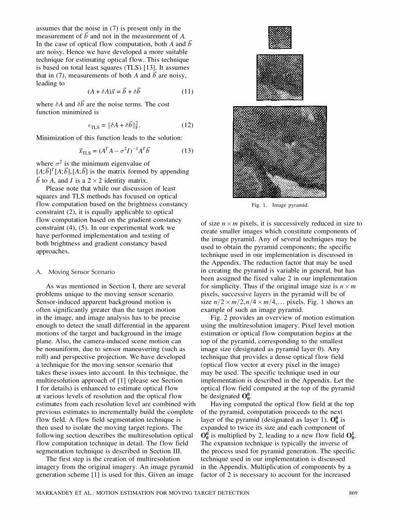
As was mentioned in Section I, there are severalproblems unique to the moving sensor scenario.Sensor-induced apparent background motion isoften significantly greater than the target motionin the image, and image analysis has to be preciseenough to detect the small differential in the apparentmotions of the target and background in the imageplane. Also, the camera-induced scene motion canbe nonuniform, due to sensor maneuvering (such asroll) and perspective projection. We have developeda technique for the moving sensor scenario thattakes these issues into account. In this technique, themultiresolution approach of [1] (please see SectionI for details) is enhanced to estimate optical flowat various levels of resolution and the optical flowestimates from each resolution level are combined withprevious estimates to incrementally build the completeflow field. A flow field segmentation technique isthen used to isolate the moving target regions. Thefollowing section describes the multiresolution opticalflow computation technique in detail. The flow fieldsegmentation technique is described in Section III.The first step is the creation of multiresolution

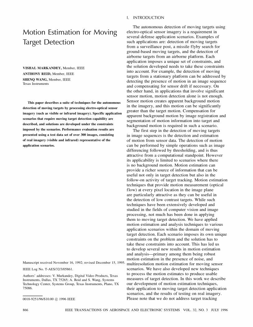
imagery from the original imagery. An image pyramidgeneration scheme [1] is used for this. Given an image

Fig. 1. Image pyramid.

of size n£m pixels, it is successively reduced in size tocreate smaller images which constitute components ofthe image pyramid. Any of several techniques may beused to obtain the pyramid components; the specifictechnique used in our implementation is discussed inthe Appendix. The reduction factor that may be usedin creating the pyramid is variable in general, but hasbeen assigned the fixed value 2 in our implementationfor simplicity. Thus if the original image size is n£mpixels, successive layers in the pyramid will be ofsize n=2£m=2,n=4£m=4, : : : pixels. Fig. 1 shows anexample of such an image pyramid.Fig. 2 provides an overview of motion estimation

using the multiresolution imagery. Pixel level motionestimation or optical flow computation begins at thetop of the pyramid, corresponding to the smallestimage size (designated as pyramid layer 0). Anytechnique that provides a dense optical flow field(optical flow vector at every pixel in the image)may be used. The specific technique used in ourimplementation is described in the Appendix. Let theoptical flow field computed at the top of the pyramidbe designated O00.Having computed the optical flow field at the top

of the pyramid, computation proceeds to the nextlayer of the pyramid (designated as layer 1). O00 isexpanded to twice its size and each component ofO00 is multiplied by 2, leading to a new flow field O

10.

The expansion technique is typically the inverse ofthe process used for pyramid generation. The specifictechnique used in our implementation is discussedin the Appendix. Multiplication of components by afactor of 2 is necessary to account for the increased

MARKANDEY ET AL.: MOTION ESTIMATION FOR MOVING TARGET DETECTION 869

Fig. 2. Multiresolution optical flow computation.

pixel resolution with respect to the previous pyramidlayer.O10 is used to warp the second image at layer

1 of the pyramid towards the first image. Warpingis performed on a pixel-by-pixel basis. The specifictechnique used in our implementation utilizes imageinterpolation to achieve subpixel accuracy. Detailsof the technique are provided in the Appendix.Residual optical flow is then computed between thefirst image of layer 1 and the warped image. Let thisvector field be called O01. The sum of O10 and O

01

provides a complete estimate of optical flow at layer1. Computation then moves to the next lower layer ofthe pyramid. The optical flow field from the previouslayer is expanded to twice its size, each componentmultiplied by 2, and the above steps are repeated.This computation is continued until the bottom of thepyramid, corresponding to the original image size, isreached. The optical flow field available at this pointhas been incrementally computed, with contributionsfrom each level of the pyramid. Let this flow fieldbe represented in terms of its component arrays as(U,V). This flow field may then be subjected to furtherprocessing, such as segmentation, to isolate regionscorresponding to moving targets. A segmentationtechnique is described in Section III.

III. USING MOTION ESTIMATES FOR MOVINGTARGET DETECTION

Having computed the motion estimates by oneof the gradient-based methods discussed above, thenext step in moving target detection is the processingof these motion estimates to generate a list of targetdetections. Next we present a technique to realize thisfunctionality for imagery acquired from a stationarysensor (sensor may have some drift). A technique forthe case of moving sensors is presented in SectionIIIB.

A. Stationary Sensor Scenario

Given the optical flow field consisting of estimates(u,v) at every pixel location, a measure of motionenergy in a pixel neighborhood is estimated byconsidering a circular region centered at that pixel andcomputing the sum of contributions from individualoptical flow components in the region. For a givenpixel location, the average motion energy computedfrom the surrounding circular region is

E =1N

NXi=1

(u2i + v2i ) (14)

where the index i specifies individual pixel location inthe region, and N is the total number of pixels in thecircular region of summation. A circular summationregion is used to account for the fact that the directionof target motion is not known a priori. The target mayhave purely lateral motion, it may be moving towardsor away from the sensor, or it may skew or swerve withrespect to the sensor. The nondirectional nature of thecircular region makes it a robust choice to account forthis possible variability in target motion.The value E computed above is assigned as the

score for the region. Regions are ranked according totheir motion energy scores and a cascade algorithmdeveloped in earlier work [8] is used for regionmerging and splitting before the final list of potentialmoving target regions is generated. The final outputis a ranked target list. Its content includes candidatemoving target regions with associated statisticssuch as region centroids, size estimates, confidencemeasures in relative motion scale, etc. Any usefulauxiliary information in the motion analysis can betabulated here for on-line study. The default numberof candidate regions on the list is set at ten whichmeets the requirements specified in many realapplications.

870 IEEE TRANSACTIONS ON AEROSPACE AND ELECTRONIC SYSTEMS VOL. 32, NO. 3 JULY 1996

B. Moving Sensor Scenario

The technique described above for motion analysisand target list generation is primarily suitable forstationary sensors, or sensors that may have somedrift. It is not suitable for moving sensors as it relieson detecting motion energy, and will pick up thesensor-induced apparent background motion. Wehave developed a separate technique for the caseof moving sensors. This new technique is generalenough that it can handle the case of stationarysensors also, but it is more computationally complexthan the technique described above for stationarysensors. Hence, from a computational standpoint, theabove technique is attractive when it is known that thesensor is stationary. The new technique is based onthe detection of discontinuities in optical flow fields,arising due to the presence of moving targets. Thetechnique consists of the following stages.1) Discontinuity Detection: Given the optical

flow field (U,V), we first compute spatial derivativesof its component arrays, (Ux,Uy,Vx,Vy), where (x,y)are spatial image coordinates. Any of various finitedifferencing methods may be used for the spatialderivative computation. Our implementation computesthese spatial derivatives by convolving the (U,V) arrayswith spatial derivatives of 2D Gaussians.2) Initialization: Blob detection is performed on

the spatial derivative arrays (Ux,Uy,Vx,Vy). A blob arrayis initialized and for a given pixel location, if any of thespatial derivative arrays has a value above a threshold,then the blob array is assigned a value of 1 for thatpixel location, otherwise the blob array is assigned avalue of 0 for that pixel location. After the blob arrayhas been thus assigned values for all pixel locations,the next step of labeling is invoked.3) Labeling: Given the blob array from the blob

detection step, blob regions are formed by checkingthe spatial connectivity of each pixel marked 1 inthe blob array to other pixels marked 1. If a pixel ismarked 1 and so is a neighboring pixel, then they areboth assigned the same label. If a pixel has a valueof 1 in the blob array but is spatially distinct fromthe previous pixels with value 1, then the blob labelcounter is incremented and it is assigned a new label.At the end of this step, every pixel of the blob arraythat was assigned a value of 1 in the previous step willhave a label associated with it. Spatially contiguouspixels that had values of 1 in the previous step willhave the same label, while spatially distinct sets ofsuch pixels will have different labels. The label mapthus formed is then passed to the next step ofmerging.4) Merging: Blob size and spatial proximity

constraints are used to combine spatially proximateblobs. This step is used to eliminate regions of small,spatially fragmented blobs. The blobs thus created aresubjected to the next step of abstraction.

Fig. 3. Stationary sensor.

5) Abstraction: The minimum and maximumspatial coordinates for a blob of each label specifythe bounding box coordinates of that blob. Thesecoordinates can be used to compute the centroid ofthe target detection corresponding to that blob. Atarget list is created consisting of each such targetdetection centroid, bounding box dimensions, and aconfidence measure for the detection. The confidencemeasure is the average value of the strength of thespatial derivatives of the optical flow field within thebounding box.

IV. EVALUATION RESULTS

In this section we present results of experimentaltesting of the techniques described in the abovesections. Real data (visible and infrared) representativeof application scenarios was used to perform thetesting.1) Stationary Sensor Scenarios: Here we describe

tests for the case of moving target detection from astationary sensor. The results of our first experimentare shown in Fig. 3. Infrared imagery (8—12 ¹m)was used in this experiment. Two moving targets arepresent in the field of view. Target 2 begins to enterthe field of view of the sensor in the second image.Although only a portion of target 2 is visible in thesecond image, it is detected by the algorithm.The results of our second experiment are presented

in Fig. 4. The imagery in this experiment is alsoinfrared (8—12 ¹m). This experiment tests thelong-range target detection capability of our technique.A stationary as well as a moving target are present inthe field of view. The technique correctly detects themoving target in all frames except the 12th where itis completely obscured behind the stationary target.The moving target reappears in the 13th frame and thetechnique locks-on to it immediately.Results of 10 other experiments are presented in

Table I. Each experiment used a sequence of multiple

MARKANDEY ET AL.: MOTION ESTIMATION FOR MOVING TARGET DETECTION 871

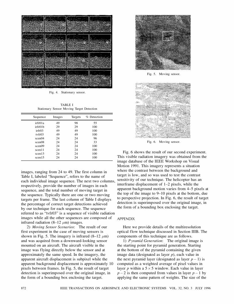
Fig. 4. Stationary sensor.

TABLE IStationary Sensor Moving Target Detection

Sequence Images Targets % Detection

irfr01a 49 98 55irfr01b 29 29 100irfr03 49 49 100tvfr03 49 49 100scen04 24 24 96scen08 24 24 33scen09 24 24 100scen11 24 24 100scen13 24 24 100scen15 24 24 100

images, ranging from 24 to 49. The first column inTable I, labeled “Sequence”, refers to the name ofeach individual image sequence. The next two columns,respectively, provide the number of images in eachsequence, and the total number of moving target inthe sequence. Typically there are one or two movingtargets per frame. The last column of Table I displaysthe percentage of correct target detections achievedby our technique for each sequence. The sequencereferred to as “tvfr03” is a sequence of visible radiationimages while all the other sequences are composed ofinfrared radiation (8—12 ¹m) images.2) Moving Sensor Scenarios: The result of our

first experiment in the case of moving sensors isshown in Fig. 5. The imagery is infrared (8—12 ¹m)and was acquired from a downward-looking sensormounted on an aircraft. The aircraft visible in theimage was flying directly below the sensor and atapproximately the same speed. In the imagery, theapparent aircraft displacement is subpixel while theapparent background displacement is approximately 10pixels between frames. In Fig. 5, the result of targetdetection is superimposed over the original image, inthe form of a bounding box enclosing the target.

Fig. 5. Moving sensor.

Fig. 6. Moving sensor.

Fig. 6 shows the result of our second experiment.This visible radiation imagery was obtained from theimage database of the IEEE Workshop on VisualMotion 1991. This imagery represents a situationwhere the contrast between the background andtarget is low, and so was used to test the contrastsensitivity of our technique. The helicopter has aninterframe displacement of 1—2 pixels, while theapparent background motion varies from 4—5 pixels atthe top of the image to 9—10 pixels at the bottom, dueto perspective projection. In Fig. 6, the result of targetdetection is superimposed over the original image, inthe form of a bounding box enclosing the target.

APPENDIX

Here we provide details of the multiresolutionoptical flow technique discussed in Section IIIB. Thecomponents of this technique are as follows.1) Pyramid Generation: The original image is

the starting point for pyramid generation. Startingat the bottom of the pyramid containing the givenimage data (designated as layer p), each value inthe next pyramid layer (designated as layer p¡ 1) iscomputed as a weighted average of pixel values inlayer p within a 5£ 5 window. Each value in layerp¡2 is then computed from values in layer p¡ 1 byapplying the same pattern of weights. The size of the

872 IEEE TRANSACTIONS ON AEROSPACE AND ELECTRONIC SYSTEMS VOL. 32, NO. 3 JULY 1996

weighting function is not critical and a 5£ 5 patternis used because it provides adequate filtering at lowcomputational cost. The weight values are selected toprovide an approximation to Gaussian filtering. Thefiltering operation can be represented as

Ik¡1(i,j) =2X

m=¡2

2Xn=¡2

w(m,n)Ik(2i+m,2j+n)

(15)

where Ik(i,j) is the image intensity at pixel location(i,j) in layer k of the pyramid, and w(m,n) is theweighting function.2) Optical Flow Field Computation: Any optical

flow computation technique that provides flowestimates at pixel level resolution may be used.Examples are several techniques based on thebrightness, and gradient constancy assumptions [2—7,9], and techniques based on correlation or Fouriertransform based techniques [1]. The technique used inour implementation is based on the gradient constancyassumption and computes the optical flow estimate(u,v) at every pixel by solving the following equations:

Ixxu+ Ixyv+ Ixt = 0 (16)

Ixyu+ Iyyv+ Iyt = 0 (17)

where the terms Ixx, : : : ,Iyt represent spatio-temporalderivatives of image intensity.3) Expansion: Expansion is the inverse of the

filtering operation used to generate the image pyramiddescribed in Section IIIB. Expansion from layer k¡ 1to layer k of the pyramid is achieved by

Ik(i,j) =2X

m=¡2

2Xn=¡2

w(m,n)Ik¡1

μi¡m2,j¡ n2

¶(18)

where Ik(i,j) is the image intensity at pixel location(i,j) in layer k of the pyramid, and w(m,n) is theweighting function. Note that this weighting functionis the same as that used for pyramid generation. Onlyterms for which (i¡m)=2 and (j¡ n)=2 are integersare used in the above sum.4) Warping: Given an image pair I1 and I2 and

the optical flow field O between them, the purposeof image warping is to warp I2 back in the directionof I1 on a pixel-by-pixel basis using the flow fieldcomponents of O. This is achieved by creating a newimage I2:

I2(x,y) = I2(x+ u±t,y+ v ±t) (19)

where (u,v) represents the optical flow vector atlocation (x,y), and ±t is the time interval betweenimage frames I1 and I2. Note that as the vectorcomponents (u,v) are typically real valued, the

quantities x+ u±t, y+ v ±t may not correspondto integer pixel locations. In such cases, bilinearinterpolation is used to compute the image intensityvalues.

REFERENCES

[1] Burt, P. J., et al. (1989)Object tracking with a moving camera.In Proceedings of the Workshop on Visual Motion, IEEE,1989.

[2] Cornelius, N., and Kanade, T. (1986)Adapting optical-flow to measure object motion inreflectance and X-ray image sequences.In N. I. Badler and J. K. Tsotsos (Ed.), Motion:Representation and Perception.Amsterdam: North-Holland Press, 1986.

[3] Gennert, M. A., and Negahdaripour, S. (1987)Relaxing the brightness constancy assumption incomputing optical flow.Memo 975, MIT AI Lab, 1987.

[4] Girosi, F., Verri, A., and Torre, V. (1989)Constraints for the computation of optical flow.In Proceedings of the Workshop on Visual Motion, 1989.

[5] Horn, B. K. P., and Schunck, B. G. (1981)Determining optical flow.In J. M. Brady (Ed.), Computer Vision.Amsterdam: North-Holland Publishing, 1981.

[6] Kearney, J. K. (1983)Gradient-based estimation of optical flow.Ph.D. dissertation, Dept. Computer Science, University ofMinnesota, Minneapolis, 1983.

[7] Koch, C., et al. (1989)Computing optical flow in resistive networks and in theprimate visual system.In Proceeding of the Workshop on Visual Motion, 1989.

[8] Merickel, M. B., Lundgren, J. C., and Shen, S. S. (1984)A spatial processing algorithm to reduce the effects ofmixed pixels and increase the separability between classes.Pattern Recognition, 17, 5 (1984), 525—533.

[9] Mitiche, A. (1984)Computation of optical flow and rigid motions.In Proceedings of the Workshop on Computer Vision:Representation and Control, 1984.

[10] Russo, P., Markandey, V., Bui, T. H., and Shrode, D. (1990)Optical flow techniques for moving target detection.In Proceedings of Sensor Fusion III: 3-D Perception andRecognition, SPIE, 1990.

[11] Schunck, B. G. (1988)Image flow: Fundamentals and algorithms.In W. N. Martin and J. K. Aggarwal (Eds.), MotionUnderstanding–Robot and Human Vision.Boston: Kluwer Academic Publishers, 1988.

[12] Tretiak, O., and Pastor, L. (1982)Velocity estimation from image sequences with secondorder differential operators.In Proceedings of the International Conference on PatternRecognition, 1982.

[13] Van Huffel, S., and Vandewalle, J. (1985)The use of total linear least squares techniques foridentification and parameter estimation.1985, 1167—1172.

[14] Wohn, K., Davis, L. S., and Thrift, P. (1983)Motion estimation based on multiple local constraints andnonlinear smoothings.Pattern Recognition, 16, 6 (1983).

MARKANDEY ET AL.: MOTION ESTIMATION FOR MOVING TARGET DETECTION 873

Vishal Markandey (S’84–M’90) received a Bachelor’s degree in electronics andcommunications engineering from Osmania University, India, in 1985, and aMaster’s degree in electrical engineering from Rice University, Houston, TX, in1988.He is a Senior Member of the Technical Staff and Team Leader of the

Advanced Video Systems Team in Texas Instruments’ Digital Imaging CorporateVenture Project. He is responsible for the development of algorithms andarchitectures for video products based on the Digital Micromirror Device.Mr. Markandey is a member of the Society of Motion Picture and Television

Engineers.

Anthony Reid (M’81) received his B.S.E.E. degree (cum laude) from RensselaerPolytechnic Institute, Troy, NY, in 1970, the M.S.E.E. degree from StanfordUniversity, Stanford, CA, in 1971, and the Ph.D. degree from Southern MethodistUniversity, Dallas, TX, in 1994.His engineering career started at Sandia Laboratories, Livermore, CA as

an MTS doing survivability analysis of U.S. strategic nuclear defense systems.Later, he was an MTS at AT&T Bell Labs, Indian Hill, IL doing system design,development and analysis of digital communication synchronization receivers,and fault-tolerant time division networks for long distance call switching. Priorto joining Texas Instruments (TI), he was a Senior Research Scientist withR. R. Donnelly and Sons, Chicago, IL. He joined TI in 1984 where he is now aSenior MTS and Branch Manager of Advanced Signal Processing in the SystemsTechnology Center of the Advanced Technology Entity in Systems Group.

Sheng Wang (M’79) received the B.S. degree from National Chiao TungUniversity, Hsinchu, Taiwan, in 1970, the M.S. degree from University ofConnecticut, Storrs, in 1974, and the Ph.D. degree from State University of NewYork, Buffalo, in 1979, all in electrical engineering.From 1979 until 1982, he was an Imaging Scientist at Picker International, Inc.,

Cleveland, OH. In February 1982, he joined Bell Labs, Indianapolis, IN as anMTS at the Advanced Communications Laboratory. Since May 1984, he has beenwith Texas Instruments, Inc. and is currently a member of the Group TechnicalStaff at TI Systems Group. His main interests are in the signal processing area,in particular, DSP applications, image sequence analysis, target tracking, andmultiresolution analysis.

874 IEEE TRANSACTIONS ON AEROSPACE AND ELECTRONIC SYSTEMS VOL. 32, NO. 3 JULY 1996