0011226
TRANSCRIPT
8/14/2019 0011226
http://slidepdf.com/reader/full/0011226 1/32
a r X i v : h e p - t h / 0 0 1 1 2 2 6 v 1 2
4 N o v 2 0 0 0
hep-th/0011226CTP-MIT-3044UUITP-11/00
Gauge Fields and Fermions in Tachyon Effective Field Theories
Joseph A. Minahan1
Department of Theoretical PhysicsBox 803, SE-751 08 Uppsala, Sweden
andBarton Zwiebach2
Center for Theoretical PhysicsMassachusetts Institute of Technology
Cambridge, MA 02139, USA
Abstract
In this paper we incorporate gauge fields into the tachyon field theory models for un-stable D-branes in bosonic and in Type II string theories. The chosen couplings yieldmassless gauge fields and an infinite set of equally spaced massive gauge fields on codi-mension one branes. A lack of a continuum spectrum is taken as evidence that the stabletachyon vacuum does not support conventional gauge excitations. For the bosonic stringmodel we find two possible solvable couplings, one closely related to Born-Infeld forms andthe other allowing a detailed comparison to the open string modes on bosonic D-branes.We also show how to include fermions in the type II model. They localize correctly onstable codimension one branes resulting in bose-fermi degeneracy at the massless level.Finally, we establish the solvability of a large class of models that include kinetic termswith more than two derivatives.
1E-mail: [email protected] E-mail: [email protected]
1

8/14/2019 0011226
http://slidepdf.com/reader/full/0011226 2/32
Contents
1 Introduction and summary 2
2 Coupling gauge fields to the superstring tachyon model 6
2.1 The superstring model revisited . . . . . . . . . . . . . . . . . . . . . . . . 7
2.2 Coupling to gauge fields . . . . . . . . . . . . . . . . . . . . . . . . . . . . 8
3 Coupling gauge fields to the bosonic string tachyon model 11
3.1 The bosonic string model revisited . . . . . . . . . . . . . . . . . . . . . . 12
3.2 Coupling to gauge fields . . . . . . . . . . . . . . . . . . . . . . . . . . . . 13
3.3 An alternative coupling to gauge fields . . . . . . . . . . . . . . . . . . . . 14
4 Comparison to the bosonic D-brane spectrum 17
5 Fermion fields in the superstring tachyon model 20
6 Higher derivative actions in the superstring tachyon model 22
6.1 Higher derivative actions . . . . . . . . . . . . . . . . . . . . . . . . . . . . 22
6.2 Gauge fluctuations for the modified Born-Infeld action . . . . . . . . . . . 25
6.3 Higher codimension branes . . . . . . . . . . . . . . . . . . . . . . . . . . . 26
7 Conclusions 27
1 Introduction and summary
While the complete understanding of Sen’s conjectures on tachyon condensation and D-
brane annihilation [1] is likely to require the full use of string field theory, simplified
field theory models of tachyon dynamics are a useful tool in describing some aspects of
this dynamics in a simpler context. In the familiar cubic version of open string field
theory [2] (and its nonpolynomial extension to open superstring field theory [3]) the
phenomenon of tachyon condensation is really a condensation of a string field ; the tachyon,
along with an infinite number of scalar modes acquire expectation values [4, 5, 6]. Onthe other hand, in boundary string field theory (B-SFT) [7, 8] – a much less developed
version of string field theory incorporating a certain degree of background independence,
tachyon condensation involves the tachyon field alone. Indeed, we proposed two models of
tachyon dynamics [9, 10] that anticipated the exact tachyon potentials that emerge from
2
8/14/2019 0011226
http://slidepdf.com/reader/full/0011226 3/32
analysis of B-SFT for both the open bosonic string and the open superstring respectively
[11, 12, 13, 14]. Our models were derived by taking an ℓ → ∞ limit of tachyon models
[15] whose spectrum around soliton solutions are governed by reflectionless Schroedinger
potentials U ℓ = ℓ2 − ℓ(ℓ + 1)sech2(x).3
We included gauge fixed dynamics in the open bosonic string model of ref. [9]. These
interactions, inspired by those of cubic string field theory considered in [18], give the
expected results for the gauge field spectrum on the brane represented by a lump solution.
Nevertheless, recent results in B-SFT including gauge fields [19, 20, 21, 22, 23] indicate
that simpler gauge invariant interactions would also represent the physics quite accurately.
One of the objectives of the present paper is to introduce into both the bosonic string and
the superstring tachyon models gauge invariant interactions that preserve solvability and
lead to localized gauge invariant dynamics on the world volume of solitons representing
lower dimensional branes. Again, much of our insight is based on the behavior of finiteℓ models. Happily, our results are consistent with the general (Born-Infeld type) forms
discussed in [19, 20, 21, 22, 23].
We will show that the gauge interactions in the superstring model lead to a discrete
spectrum for the gauge fluctuations on the tachyon background representing the codimen-
sion one brane. In particular we find no continuum sector. The masses for the fluctuations
match the masses found for the tachyon fluctuations. The coupling of the gauge fields is of
the form exp(−T 2/2)F 2µν . Since the tachyon vacuum is at T = ±∞ one may ask, as usual,
whether the gauge field has dynamics on this vacuum. While the factor multiplying this
gauge field is going to zero, suggesting that the gauge field becomes nondynamical and
acts as a Lagrange multiplier that sets the associated currents to zero [24], this vanishing
prefactor could alternatively be taken as a sign of strong coupling dynamics [25, 26] in
which case the fate of the gauge field is less clear. We think, however, that the proof of
gauge field localization on the codimension one brane, as evidenced by the discrete spec-
trum of gauge field fluctuations without a continuum, implies that the tachyonic vacuum
does not support conventional local gauge field excitations. This is because the asymp-
totic regions of the codimension one brane live on the tachyon vacuum, and particle-like
gauge fluctuations around this vacuum would have manifested themselves as a continuum
spectrum of fluctuations of the gauge field around the lump solution.
For the bosonic case, we discuss two plausible gauge interaction terms. In the first one,
arising from a Born-Infeld action, we find a discrete spectrum, where the spacing between3For a pedagogical review on these and other solvable Hamiltonians with references to the early
literature see [16]. Applications of reflectionless systems to fermions can be found in [17].
3
8/14/2019 0011226
http://slidepdf.com/reader/full/0011226 4/32
levels is twice the spacing for the tachyon fluctuations. For the second one the tachyon
prefactor in front of the gauge kinetic term is the same as that for the tachyon kinetic term.
Here we find that the level spacing matches those of the tachyon fluctuations. This second
form of the coupling does not appear to have a solvable finite ℓ counterpart. Nevertheless,the correctness of the mass level spacing leads us to believe that this is the coupling chosen
in string theory. The bosonic Born-Infeld action was considered in the recent papers of
Cornalba [19], Okuyama [20], Andreev [21] and Tseytlin [23]. In particular, Andreev [21]
discussed the possibility of ambiguities in such actions. The second form was actually
advocated by Gerasimov and Shatashvili [22], as a natural choice of coordinates in the
space of boundary interactions. While it seems likely that the two actions considered here
would be related by a field redefinition in the context of an extended full theory including
all higher derivatives, the truncations they represent do give different spectra.
Indeed, we use the spectrum associated to this second coupling to demonstrate how
the fluctuation modes for the tachyon and gauge fields compare with open string states
on bosonic D branes. In a complete string field theory model of tachyon condensation it is
not enough to show that there is a discrete spectrum about the lump solutions. One must
also account for the huge degeneracies that occur at the higher mass levels. In a theory
with just a tachyon, there are no degenerate states at higher mass levels. If other fields
are introduced, however, they too have fluctuations about the lump and modes can be
degenerate. Moreover, an interesting and highly suggestive pattern emerges. The massless
gauge field in the bulk localizes to a massless gauge field on the codimension one brane,
with no extra massless scalar, as opposed to the case of Kaluza-Klein reduction, where
a massless scalar accompanies the lower dimensional gauge field. String theory, however,
still has this massless scalar, and in our framework it arises as a fluctuation mode of the
tachyon field, the mode representing the translation of the brane. Such a pattern appears
to repeat at higher mass levels and we believe it is generic: modes removed through
localization reappear as fluctuation modes for lower mass fields. In light of these remarks,
we now see that the equally spaced mass levels of the original tachyon models are more
than just suggestive patterns. These patterns are necessary in order for the models to
reproduce the full open string spectrum on a D-brane when additional fields are included.
The result, with proper account of higher derivatives, is presumably B-SFT with all fields.
We also explore the coupling of fermions to the tachyon model of the superstring.
Thus we include, along with the tachyon and the gauge field, the Majorana spinor present
in the (unstable) D9 brane of IIA. We propose certain couplings of the tachyon field to the
4

8/14/2019 0011226
http://slidepdf.com/reader/full/0011226 5/32
fermions that result in rather desirable properties. Namely, half of the fermionic degrees
of freedom localize on the kink solution representing the D8, giving rise to a massless
spectrum consistent with supersymmetry. The massive fermion spectrum is calculable
and the mass squared spacing is the expected one. No continuum spectrum arises andthe fermion becomes infinitely massive at the stable tachyonic vacuum.
Finally, we explore how higher derivative terms affect the solvability of the models.
Focusing on the model relevant to the superstring we replace the derivative term ∂T∂T by
a general function f (∂T∂T ) where f ′(0) = 0, and show that solvability is preserved while
the precise values for the mass spacings and ratios of tensions between branes are altered.
In particular, judicious choices of the form of f allow us to obtain (solvable) Born-Infeld
type actions. In particular we study a Born-Infeld type action proposed by Garousi [27]
and Bergshoeff et.al. [28] where the tachyon kinetic term is insider the Born-Infeld square
root. Such an action was argued to be consistent with open string scattering amplitudes
and T duality. We will find that this action has a kink solution with vanishing width.
In addition, we find that the fluctuations for the tachyon field have the correct spacing
between mass levels, although the spacings for gauge fluctuations is half the expected
amount.
We will also see that higher derivative terms can lead to regular solutions for higher
codimension branes. For example, with higher derivative terms there can be even codi-
mension branes which are tachyon solitons of the world volume theory of several D9
brane-antibrane pairs of type IIB. Likewise, there can be odd codimension branes which
are solitons of the world-volume theory of several unstable D9 branes of type IIA. In
agreement with the observations of [13] such solutions do not appear to require expecta-
tion values for the gauge fields. The kinetic form of the tachyon field allows finite energy
configurations even though the asymptotic values of the tachyon wind over the sphere at
infinity.
We find it striking just how simple it is for the tachyon to induce complete localization
for the gauge fields and fermions on the brane. From the viewpoint of solitons, we see that
the complete localization of the tachyon relies on the absence of tachyon dynamics at the
stable vacuum, something directly guaranteed by the form of the tachyon potential. This
implies that the spectrum around the configuration representing the brane cannot have
a continuum sector arising from the tachyon field. This results in a soliton spectrum of
stringy type. Indeed, with the fluctuation spectrum governed by a Schroedinger potential
with no continuous spectrum one must necessarily have an infinite number of energy
levels. The complete localization of gauge fields and fermions follows by couplings to the
5
8/14/2019 0011226
http://slidepdf.com/reader/full/0011226 6/32
localized tachyon. Again, these fields give rise to an infinite number of fields on the soliton.
We find it quite remarkable that all this is exactly modeled with simple interactions of a
scalar field, a gauge field and a fermion.
This paper is organized as follows. In section 2 we show how to include gauge fields
through gauge invariant interactions for general classes of models with stable kinks, which
include the two derivative truncation of the unstable D9 brane in type IIA. In section 3
we do a similar analysis for models with unstable lumps, which include the two derivative
truncation for the tachyon effective field theory in bosonic string theory. In section 4
we compare the results for the bosonic gauge fluctuations to that of the bosonic string.
Here, we are able to match the fluctuation modes to particular open string oscillator
states. In section 5 we discuss the inclusion of fermion fields in the models with kinks.
Finally in section 6 we consider the extension of the tachyon superstring model where we
include certain kinds of higher derivative terms (this class includes the modified Born-
Infeld action). We then use such actions to obtain nontrivial solutions representing branes
of codimension higher than one. Concluding remarks are offered in section 7.
2 Coupling gauge fields to the superstring tachyon
model
In Ref. [9], gauge fixed interactions were added to the bosonic tachyon effective field theory
corresponding to the ℓ = ∞ model, and to the finite ℓ models. Such interactions wereinspired by similar terms appearing in gauge fixed cubic string field theory, and had been
considered in [18]. The interactions were tailored to result in gauge fields localized on the
tachyon solutions representing lower dimensional branes. The spectrum of massive gauge
excitations could be solved exactly and were shown to have equally spaced levels, with
the correct spacing. Nevertheless, it is now clear that in boundary string field theory one
should naturally be led to a gauge invariant description of the interactions. Indeed, the
forms of such interactions have recently been discussed by several authors [19, 20, 21].
In light of this, we look, for gauge invariant interactions of a gauge field with the
tachyon field that lead to integer spacings for the gauge fluctuations, a residual gaugeinvariance on the solitons or lumps and absence of conventional degrees of freedom for
the gauge field in the vacuum. There are remarkably simple actions that posess these
features for both the bosonic model and the superstring model. In this section we will
discuss the case of the superstring model while in section 3 will discuss the case of the the
6

8/14/2019 0011226
http://slidepdf.com/reader/full/0011226 7/32
bosonic string model. In both cases it will be instructive to consider the finite ℓ models
whose limit ℓ → ∞ led to the string models.
2.1 The superstring model revisited
Our construction will be quite general, allowing us to specialize to various models, such as
the finite ℓ models discussed in [9], or to the harmonic oscillator model which is reached
by taking the ℓ → ∞ limit and which leads directly to the two derivative truncation
of boundary string field theory. As shown in [10], these models can be constructed in
generality by reconstructing the field theory from the profile of the kink solution. Indeed,
given a kink profile
φ(x) = K(x), (2.1)
where K(x), for kink4
, is either a monotonically increasing or a monotonically decreasingfunction of the coordinate x ∈ [−∞, ∞], the desired field theory is given by:
S = −
dtd p+1xK′(T )2
(∂T )2 + 1
, (2.2)
where the prime denotes partial derivative with respect to the argument, the scalar field
T is related to φ as
φ = K(T ) , (2.3)
and the kink is just
T (x) = x . (2.4)The action (2.2), assuming K′′(0) = 0, has a vacuum at T = 0 where there is a tachyon
of mass squared
M 2T =K′′′(0)
K′(0), (2.5)
In addition, one easily confirms that
√2
2π
T kink
T =
√2
π
∞
−∞
dx K′(x)
K′(0)
2, (2.6)
where T denotes the tension of the spacefilling brane represented by the T = 0 vacuumof (2.2) and T kink is the tension of the (codimension one) kink. In string theory the above
ratio is one.
4In [10] we used the variable P , for profile, rather than K. We have changed notation to be able tocall the lump profiles L(x).
7
8/14/2019 0011226
http://slidepdf.com/reader/full/0011226 8/32
For example the finite ℓ models can be obtained by taking
K′ℓ(x) =√
T sechℓ(x) . (2.7)
The spectrum of fluctuations around the kink solutions of these models are governed by
a Schroedinger equation with potential [9]
U ℓ(x) = ℓ2 − ℓ(ℓ + 1)sech2(x) . (2.8)
We now consider the fluctuation problem around the kink solution T (x) = x. For this
purpose, we let T → x + T in (2.2), where T represents the fluctuation field. It is then
useful to redefine the fluctuation field as
K′(x) T = T . (2.9)
Up to quadratic fluctuations and after dropping constant terms, the action is
S quad = −
dtd pydx
∂ µ T ∂ µ T + T − ∂ 2
∂x2+
K′′′(x)
K′(x)
T
. (2.10)
The p+2 indices µ have been split into p+1 indices µ along the brane worldvolume (t, yi),
and the index x along the coordinate transverse to the brane. From the above equation
it follows that the Schroedinger problem for the tachyon fluctuations is simply
− d
2
dx2 T + K′′′
(x)K′(x) T = M 2 T . (2.11)
The reader can verify that with Kℓ given in (2.7) the potential term in the above equation
equals U ℓ ((2.8)). It is also clear from the above equation that T 0(x) = K′(x) is a solution
with M 2 = 0. This is the translation mode of the kink in the original field variable. Indeed,
from (2.3), (2.4) and (2.9) we have φ = K(x + ǫ T 0(x)/K′(x)) = K(x) + ǫK′(x) + O(ǫ2).
Since K(x) is monotonic, K′(x) does not have zeroes. Therefore, K′(x) is the ground state
wavefunction for the Schroedinger equation in (2.11) and thus there are no tachyonic
fluctuations.
2.2 Coupling to gauge fields
In string theory, the gauge fields appear through the Born-Infeld action
S BI = −T
dtd p+1x V (T )
− det(ηµν + F µν ) , (2.12)
8
8/14/2019 0011226
http://slidepdf.com/reader/full/0011226 9/32
where V (T ) is the tachyon potential. Here, we are only interested in finding the gauge
fluctuations, so it suffices to make the approximation
− det(ηµν + F µν ) = 1 +
1
4F µν F µν
+ .... (2.13)
Therefore, the action we use for the gauge fields and tachyons is
S = −
dtd p+1xK′(T )2
(∂T )2 + 1 +1
4F µν F µν
. (2.14)
In order to see that (2.14) is a reasonable coupling we study the spectrum of fluctua-
tions of the gauge field on the background of the kink solution. We choose the axial gauge
condition
Ax = 0 , → F xµ = ∂ xAµ . (2.15)
We also note for later reference the equation of motion obtained by varying Ax, which in
the chosen gauge simplifies to
∂ µ
(K′(T ))2F xµ
= 0 → ∂ x(∂ µAµ) = 0 , (2.16)
where in the last step we have considered the reduction to linearized equations for gauge
fluctuations on the background of the tachyon kink (the tachyon expectation value is
independent of the brane coordinates). The term in the action (2.14) relevant to the
gauge field fluctuations is
S (T , A) = − dtd pydx K′(x)2 14
F µν F µν + 12
∂ xAµ∂ xAµ . (2.17)
The analysis is helped by the field redefinition
Bµ = K′(x)Aµ , F µν = ∂ µBν − ∂ ν Bµ , (2.18)
which allows us to turn (2.17) into
S (T , B(A)) = −
dtd pydx 1
4
F µν
F µν +
1
2Bµ
− ∂ 2
∂x2+
K′′′(x)
K′(x)
Bµ
. (2.19)
Comparing this last equation with (2.10) we see that the Schroedinger problem governing
the spectrum of the gauge field fluctuations on the kink is the same as that governing the
tachyon fluctuations. Just as before the ground state is associated to the wavefunction
K′(x). Note that the constant in front in (2.19) plays no special role in this or the following
analysis.
9
8/14/2019 0011226
http://slidepdf.com/reader/full/0011226 10/32
It is straightforward to understand the gauge invariance of the massless gauge mode
living on the lump solution. While we have imposed the axial gauge Ax = 0, there is still
a residual gauge invariance under
Aµ → Aµ + ∂ µε , with ∂ xε = 0 . (2.20)
This means that the field Bµ introduced in (2.18) transforms as
Bµ → Bµ + K′(x) ∂ µε . (2.21)
The massless gauge field Bµ(y) living on the brane arises as Bµ(y, x) = Bµ(y)K′(x). It
thus follows from the last equation that
Bµ(y)
→Bµ(y) + ∂ µε , ε = ε(y) , (2.22)
which is the standard gauge transformation of a gauge field. Since for this massless mode
Aµ = Bµ(y) (see (2.18)) the subsidiary field equation in (2.16) is identically satisfied.
We can also confirm that the excited wave functions arising from the Schroedinger
problem of (2.19) correspond to massive gauge fields on the brane. First note that the
action for a mode
Bµ(n)(y)ψ(n)(x) , (2.23)
where the wave function ψ(n) has eigenvalue M 2n, is of the form
dtd py 14
(F (n)µν )2 + 1
2M 2n(B(n)
µ )2 . (2.24)
In addition, the constraint (2.16), using (2.18) and (2.23), reduces to
∂ xψ(n)(x)
K′(x)
∂ µBµ(n)(y) = 0 → ∂ µBµ(n)(y) = 0 . (2.25)
The action (2.24), supplemented by this condition describes a massive gauge field.
Let us now turn to the example of the D9 brane. In [10, 13] it was argued that the
lagrangian for the tachyon field for up to two derivatives is
S = −T
dtd9x exp(−T 2/2) [∂ µT ∂ µT + 1] . (2.26)
This action can be obtained from (2.2) by setting
K′(T ) =√
T exp(−T 2/4) = limℓ→∞
Kℓ(T /√
2ℓ). (2.27)
10
8/14/2019 0011226
http://slidepdf.com/reader/full/0011226 11/32
Since by construction, K′(x) is a ground state wave function, we see that the corresponding
potential is U (x) = x2/4. Given the potential term in (2.26), the Born-Infeld action is
S BI = −T dtd9
x exp(−T 2
/2) − det(ηµν + F µν ). (2.28)
The integrand can be expanded as in (2.13) and so the fluctuation spectrum is found
using the preceding arguments. Therefore, using (2.27) and (2.19), the action for the
gauge fluctuations about the kink solution is
− T
dtd8ydx
1
4F µν F µν +
1
2Bµ
− ∂ 2
∂x2+
1
4x2 − 1
2
Bµ
. (2.29)
Hence, the fluctuation spectrum for the gauge fields is described by a harmonic oscillator,
with the lowest mode corresponding to a massless state. The spacing between the modes
is unity, which using (2.5) is twice the mass squared of the tachyon. As in (2.22) there isa residual gauge invariance for the massless vector mode on the stable 8-brane.
The absence of a continuum sector of gauge field fluctuations is manifest, and we take
this as evidence that the tachyonic vacuum does not support conventional gauge field
excitations. Indeed, in the case of scalar field excitations the logic connecting complete
localization on the brane to lack of excitations on the stable vacuum is quite direct. The
Schroedinger potential for fluctuations is U (x) = V ′′(φ(x)) = M 2ef f (φ(x)), where V is the
scalar field potential and M 2ef f denotes the effective mass of the scalar field (computed by
cancelling the linear term, if nonvanishing, with an external source). We then have that
U (x → ±∞) = M 2T where M 2T denotes the scalar field mass at the stable vacuum. Thus acontinuum arises in the Schroedinger problem for energies greater than M 2T . If M 2T → ∞there is no continuum.
3 Coupling gauge fields to the bosonic string tachyon
model
In this section we discuss the general construction for gauge fields coupled to the bosonic
string model. We will give two types of interaction terms. The first such term leads to
a solvable spectrum for all finite ℓ models. This type of interaction is derivable from the
Born-Infeld action. The second such term only has a solvable spectrum for the ℓ = ∞model. However, its spectrum is what one would expect from open string modes on D
branes in bosonic string theory. This leads us to believe that this is the choice taken by
B-SFT.
11
8/14/2019 0011226
http://slidepdf.com/reader/full/0011226 12/32
3.1 The bosonic string model revisited
We begin by describing a general construction of a scalar field theory given the profile of
a lump solution. We let
φ(x) = L(x2) (3.1)
define the lump profile. By lump, we mean a field configuration where the derivative of
the profile with respect to the coordinate x vanishes at one point. The argument of Lmanifestly incorporates an expected reflection symmetry. The equation of motion of the
lump relates the potential V in the action to the spatial derivative of the profile as follows
V (φ(x)) =1
2[ φ′(x) ]2 = 2x2[ L′(x2) ]2 . (3.2)
From (3.2) it is clear that x
L′(x2) must have one and only one zero.
We now introduce a new field φ = L(T ), which in view of (3.1) implies
T (x) = x2. (3.3)
This in turn gives V (φ) = 2T [ L′(T ) ]2. Thus, the action S = − (12
(∂φ)2+V (φ)) becomes
S = −
dtd p+1x(L′(T ))2 1
2(∂T )2 + 2T
. (3.4)
For the finite ℓ models, we have that
Lℓ(x2
) = T 2T 0
1
sechℓ−1(√T 0) sechℓ−1
(x), (3.5)
where T 0 is the value for T at the unstable vacuum, where the potential is a maximum.
The tension T is its vacuum energy.
To find the fluctuations, we let T = x2 + τ and define the fluctuation field as T =
L′(x2)τ . Up to quadratic order, the action in (3.4) becomes
S = −
dtd p+1x
1
2∂ µ T ∂ µ T +
1
2 T
− ∂ 2
∂x2+ U (x)
T
, (3.6)
where U (x) ≡ 6L′′(x2)
L′(x2)+ 4x2L′′′(x2)
L′(x2)=
1
xL′(x2)
d2
dx2(xL′(x2)). (3.7)
Hence, we see that the fluctuation spectrum is determined by the Schroedinger equation
− d2
dx2 T + U (x) T = M 2 T . (3.8)
12
8/14/2019 0011226
http://slidepdf.com/reader/full/0011226 13/32
It follows from the last equation in (3.7) that xL′(x2) is an eigenfunction with M 2 = 0,
and so is the translation mode. Since xL′(x2) has one zero, this is the first excited state
and therefore there exists one tachyonic mode.
We can now apply this general analysis to the specific case of the two derivativetruncation of boundary string field theory. In boundary string field theory it was argued
that the action for up to two derivatives for the tachyon field is [11, 12]
S = −4 eT
dtd p+1x1
2∂ µφ ∂ µφ − 1
4φ2 ln φ2
. (3.9)
This model can be obtained by taking the limit ℓ → ∞ in the finite ℓ models [9]. The
field redefinition φ = exp[−14T ] casts this action in the form:5
S T = −eT 4
dtd p+1x exp(−T /2)
1
2∂ µT ∂ µT + 2T
. (3.10)
This action has the form in (3.4), with
L′(T ) =1
2
√T e exp(−T /4), (3.11)
and hence has a codimension lump solution with T = x2. From (3.11) and (3.7) we see
that
U ∞(x) =1
4x2 − 3
2, (3.12)
hence, the fluctuation spectrum has a tachyon with m2 = −1 and higher mass states
with integer spacing, ∆m2 = 1. In [9] it was shown that the action in (3.10) also has
codimension d lump solutions with T = di (x2i /2) − 2(d − 1). In this case, the fluctuation
spectrum is governed by a d dimensional harmonic oscillator.
3.2 Coupling to gauge fields
Now let us include contributions from the gauge fields. We are again interested in the
Born-Infeld action in (2.12), but for the analysis of the fluctuation spectrum it is sufficient
to use
S = −
dtd p+1x(L′(T ))2
1
2(∂T )2 + 2T + 2T · 1
4F µν F µν
. (3.13)
To find the fluctuation spectrum about the lump solution, we choose the axial gaugeAx = 0 and let
Bµ = (2T )1/2L′(T )Aµ , F µν = ∂ µBν − ∂ ν Bµ. (3.14)5We choose to work with the form of the 2-derivative tachyon action for which the tachyon mass is
the correct one.
13
8/14/2019 0011226
http://slidepdf.com/reader/full/0011226 14/32
In terms of these fields, the part of the action containing the gauge fields becomes
S (T , B(A)) = −
dtd pydx
1
4 F µν
F µν +
1
2Bµ
− ∂ 2
∂x2+ U (x)
Bµ
, (3.15)
where U (x) is defined in (3.7). Hence, the fluctuation spectrum for the Bµ fields is
governed by the same Schroedinger equation as for the tachyon fluctuations.
Since the Schroedinger potentials are the same, it would seem that the lowest mode
for the gauge field is tachyonic. But this solution needs to be discarded, along with all
solutions that are even under x → −x. Upon inspection of (3.14), we see that Aµ ∼ 1/x
if Bµ is nonzero at x = 0, which is the case for the even parity modes. Therefore, the
integrand in (3.13) diverges as 1/x2, and so the even parity modes should be disregarded.
Hence, the lowest mode corresponds to the first excited state of the Schroedinger equation
and thus is massless.
Turning to the specific example of the two derivative truncation of B-SFT, the Born-
Infeld action has the form
− eT 4
dtd p+1x 2T exp(−T /2)
− det(ηµν + F µν ). (3.16)
This form of the action has been recently obtained in BSFT [19, 20, 21]. The overall nor-
malization in (2.12) is chosen so that the gauge kinetic term has the canonical coefficient
at the open string vacuum T = 2, and so matches the form in (3.13) with L′(T ) defined
in (3.11). Therefore, the term in (2.12) expanded to two derivatives can be written as
−
dtd pydxe−T /21
4F µν F µν +
1
2Bµ
− ∂ 2
∂x2+
1
4x2 − 3
2
Bµ
, (3.17)
where T refers to the tachyon field on the lump. Hence, the components of the gauge field
also have a fluctuation spectrum given by a harmonic oscillator.
As before, the even parity solutions need to be discarded since they correspond to
singular configurations for the gauge field Aµ. Hence the lowest mode is massless and the
spacing between mass squared levels is equal to twice the magnitude of the mass squared
term of the original tachyon.
3.3 An alternative coupling to gauge fields
The double spacing for the levels seen at the end of the last subsection seems odd and
is perhaps a consequence of our only considering contributions of up to two derivatives.
14
8/14/2019 0011226
http://slidepdf.com/reader/full/0011226 15/32
Therefore, let us also consider the gauge coupling
S ′ = −
dtd p+1x(L′(T ))21
4F µν F µν . (3.18)
This does not quite have the Born-Infeld form since it is missing a factor of 2T . Note that
this is the simplest kind of term, the same factor multiplying the tachyon kinetic term is
now multiplying the conventional gauge kinetic term.
To find the spectrum about the codimension one brane, we set T = x2 and define the
new gauge field Bµ and associated field strength to be
Bµ = L′(x2)Aµ , F µν = ∂ µBν − ∂ ν Bµ . (3.19)
Subtituting back into (3.18) we find
− dtd pydx14F µν F µν + 1
2∂ xBµ∂ xBµ + 1
2U (x)BµBµ, (3.20)
where U (x) is given by
U (x) = 2L′′(x2)
L′(x2)+ 4x2L′′′(x2)
L′(x2)=
1
L′(x2)
d2
dx2L′(x2). (3.21)
This is a different Schroedinger potential than in (3.7) and does not seem to give a solvable
spectrum for the gauge fields in the finite ℓ models.
For the ℓ = ∞ model, however, the coupling in (3.18) still gives a solvable spectrum
for the gauge fluctuations. Using the expression for L′
(T ) in (3.11), the gauge action is
S ′ = −eT 16
dtd p+1x exp(−T /2)F µν F µν . (3.22)
This form of the action has been recently advocated in [22]. Using (3.21), we have that
U (x) =1
4x2 − 1
2. (3.23)
Therefore, in contrast to the previous case, we find that the lowest mode for this harmonic
oscillator equation is massless. In fact, there is no need to throw out the even parity
modes, since these do not correspond to singular configurations for Aµ. Thus, the spacingbetween the gauge modes is the mass squared of the tachyon.
As in the superstring case, selecting a gauge imposes a constraint on the remaining
fields. Proceeding as in (2.25) one finds the constraint on the massive modes
∂ x∂ µ(exp( T /2)B(n)µ ) = 0, (3.24)
15
8/14/2019 0011226
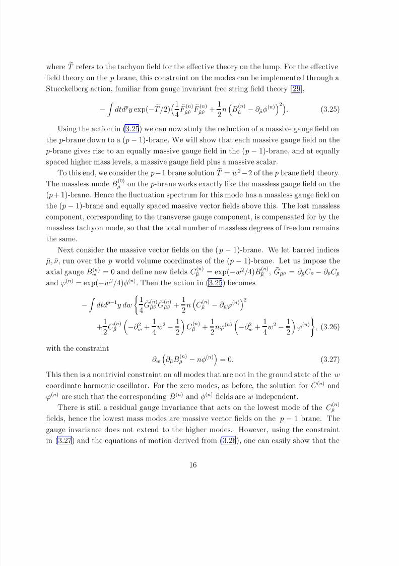
http://slidepdf.com/reader/full/0011226 16/32
where T refers to the tachyon field for the effective theory on the lump. For the effective
field theory on the p brane, this constraint on the modes can be implemented through a
Stueckelberg action, familiar from gauge invariant free string field theory [29],
−
dtd py exp(− T /2)1
4F (n)
µν F (n)
µν +1
2n
B(n)µ − ∂ µφ(n)2
. (3.25)
Using the action in (3.25) we can now study the reduction of a massive gauge field on
the p-brane down to a ( p − 1)-brane. We will show that each massive gauge field on the
p-brane gives rise to an equally massive gauge field in the ( p − 1)-brane, and at equally
spaced higher mass levels, a massive gauge field plus a massive scalar.
To this end, we consider the p−1 brane solution T = w2−2 of the p brane field theory.
The massless mode B(0)µ on the p-brane works exactly like the massless gauge field on the
( p + 1)-brane. Hence the fluctuation spectrum for this mode has a massless gauge field onthe ( p − 1)-brane and equally spaced massive vector fields above this. The lost massless
component, corresponding to the transverse gauge component, is compensated for by the
massless tachyon mode, so that the total number of massless degrees of freedom remains
the same.
Next consider the massive vector fields on the ( p − 1)-brane. We let barred indices
µ, ν , run over the p world volume coordinates of the ( p − 1)-brane. Let us impose the
axial gauge B(n)w = 0 and define new fields C
(n)µ = exp(−w2/4)B
(n)µ , Gµν = ∂ µC ν − ∂ ν C µ
and ϕ(n) = exp(−w2/4)φ(n). Then the action in (3.25) becomes
− dtd p−1y dw1
4G(n)
µν G(n)
µν + 12
n
C (n)µ − ∂ µϕ(n)2
+1
2C
(n)µ
−∂ 2w +
1
4w2 − 1
2
C
(n)µ +
1
2nϕ(n)−∂ 2w +
1
4w2 − 1
2
ϕ(n)
, (3.26)
with the constraint
∂ w
∂ µB(n)µ − nφ(n)
= 0. (3.27)
This then is a nontrivial constraint on all modes that are not in the ground state of the w
coordinate harmonic oscillator. For the zero modes, as before, the solution for C (n) and
ϕ(n) are such that the corresponding B(n) and φ(n) fields are w independent.There is still a residual gauge invariance that acts on the lowest mode of the C
(n)µ
fields, hence the lowest mass modes are massive vector fields on the p − 1 brane. The
gauge invariance does not extend to the higher modes. However, using the constraint
in (3.27) and the equations of motion derived from (3.26), one can easily show that the
16

8/14/2019 0011226
http://slidepdf.com/reader/full/0011226 17/32
higher modes satisfy the equations
− ∂ µC (n,k)µ + nϕ(n,k) = 0
−∂ µ∂ µ
C
(n,k)
ν + (n + k)C
(n,k)
ν = 0−∂ µ∂ µϕ(n,k) + (n + k)ϕ(n,k) = 0 (3.28)
where k is the mass squared arising from the wavefunctions along the y direction. Finally,
we can define a new field C (n,k)µ that is given by
C (n,k)µ = C
(n,k)µ − n
n + k∂ µϕ(n,k). (3.29)
Hence, the first and last equations in (3.28) give ∂ µ C (n,k)µ = 0. Thus, the higher modes on
the p
−1 brane have massive vectors C
(n,k)µ , and massive scalars ϕ(n,k).
4 Comparison to the bosonic D-brane spectrum
In a field theory with just a tachyon, the fluctuation modes on the unstable lump are
nondegenerate. We know of course that open string modes on D branes are highly degen-
erate. The original tachyon model, with the nice feature of having a discrete spectrum
with the correct spacing between levels, could not fail to miss most of the states that one
would expect from string theory. By adding in a gauge field, however, there are more
fluctuation modes, enough in fact to start making reasonable conjectures as to how they
match with the open strings on a D-brane.The purpose of this section is to do just that and compare the results for the tachyon
and gauge field fluctuations of the previous section to results for the D brane spectrum
in bosonic string theory. We find that our results fit nicely with a subclass of oscillator
states for the D brane fluctuations of the bosonic string. This attests to the power of
these models and strongly suggests that the original model can be made into a complete
string model by adding the rest of the fields.
In comparing the string theory construction of the spectrum on a D25-brane and
on a D24-brane, we know that (apart from momentum modes which differ) the number
of physical degrees of freedom are the same and just rearrange themselves into differentrepresentations of the Lorentz group. For example the first three levels of the D25 contain
the tachyon, a massless vector, and a massive symmetric rank two tensor respectively. On
the D24 brane, these turn into a tachyon, a massless vector and a massless scalar, and
at the next level, a massive symmetric rank two tensor, a massive vector and a massive
17
8/14/2019 0011226
http://slidepdf.com/reader/full/0011226 18/32
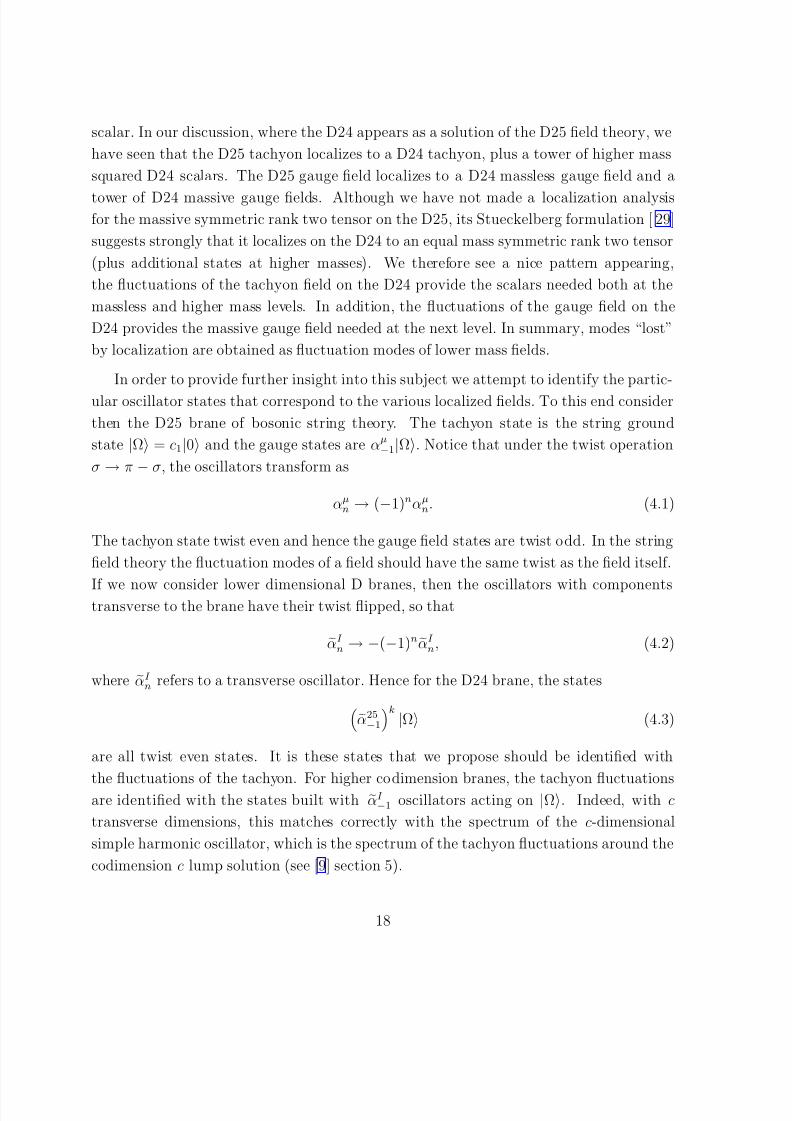
scalar. In our discussion, where the D24 appears as a solution of the D25 field theory, we
have seen that the D25 tachyon localizes to a D24 tachyon, plus a tower of higher mass
squared D24 scalars. The D25 gauge field localizes to a D24 massless gauge field and a
tower of D24 massive gauge fields. Although we have not made a localization analysisfor the massive symmetric rank two tensor on the D25, its Stueckelberg formulation [ 29]
suggests strongly that it localizes on the D24 to an equal mass symmetric rank two tensor
(plus additional states at higher masses). We therefore see a nice pattern appearing,
the fluctuations of the tachyon field on the D24 provide the scalars needed both at the
massless and higher mass levels. In addition, the fluctuations of the gauge field on the
D24 provides the massive gauge field needed at the next level. In summary, modes “lost”
by localization are obtained as fluctuation modes of lower mass fields.
In order to provide further insight into this subject we attempt to identify the partic-
ular oscillator states that correspond to the various localized fields. To this end consider
then the D25 brane of bosonic string theory. The tachyon state is the string ground
state |Ω = c1|0 and the gauge states are αµ−1|Ω. Notice that under the twist operation
σ → π − σ, the oscillators transform as
αµn → (−1)nαµ
n. (4.1)
The tachyon state twist even and hence the gauge field states are twist odd. In the string
field theory the fluctuation modes of a field should have the same twist as the field itself.
If we now consider lower dimensional D branes, then the oscillators with componentstransverse to the brane have their twist flipped, so that
αI n → −(−1)n αI
n, (4.2)
where αI n refers to a transverse oscillator. Hence for the D24 brane, the states
α25−1
k |Ω (4.3)
are all twist even states. It is these states that we propose should be identified with
the fluctuations of the tachyon. For higher codimension branes, the tachyon fluctuationsare identified with the states built with αI −1 oscillators acting on |Ω. Indeed, with c
transverse dimensions, this matches correctly with the spectrum of the c-dimensional
simple harmonic oscillator, which is the spectrum of the tachyon fluctuations around the
codimension c lump solution (see [9] section 5).
18
8/14/2019 0011226
http://slidepdf.com/reader/full/0011226 19/32
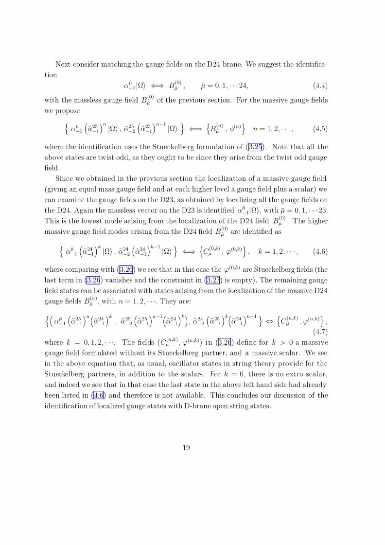
Next consider matching the gauge fields on the D24 brane. We suggest the identifica-
tion
αµ−1|Ω ⇐⇒ B
(0)µ , µ = 0, 1, · · ·24, (4.4)
with the massless gauge field B(0)µ of the previous section. For the massive gauge fields
we proposeαµ−1
α25−1
n |Ω , α25−2
α25−1
n−1 |Ω
⇐⇒
B(n)µ , φ(n)
n = 1, 2, · · · , (4.5)
where the identification uses the Stueckelberg formulation of (3.25). Note that all the
above states are twist odd, as they ought to be since they arise from the twist odd gauge
field.
Since we obtained in the previous section the localization of a massive gauge field
(giving an equal mass gauge field and at each higher level a gauge field plus a scalar) wecan examine the gauge fields on the D23, as obtained by localizing all the gauge fields on
the D24. Again the massless vector on the D23 is identified αµ−1|Ω, with µ = 0, 1, · · ·23.
This is the lowest mode arising from the localization of the D24 field B(0)µ . The higher
massive gauge field modes arising from the D24 field B(0)µ are identified as
αµ−1
α24−1
k |Ω , α24−2
α24−1
k−1 |Ω
⇐⇒
C (0,k)µ , ϕ(0,k)
, k = 1, 2, · · · , (4.6)
where comparing with (3.26) we see that in this case the ϕ(0,k) are Stueckelberg fields (the
last term in (3.26) vanishes and the constraint in (3.27) is empty). The remaining gauge
field states can be associated with states arising from the localization of the massive D24
gauge fields B(n)µ , with n = 1, 2, · · ·. They are:
αµ−1
α25−1
nα24−1
k, α25
−2
α25−1
n−1α24−1
k, α24
−2
α25−1
kα24−1
n−1 ⇔ C (n,k)µ , ϕ(n,k)
,
(4.7)
where k = 0, 1, 2, · · ·. The fields (C (n,k)µ , ϕ(n,k)) in (3.26) define for k > 0 a massive
gauge field formulated without its Stueckelberg partner, and a massive scalar. We see
in the above equation that, as usual, oscillator states in string theory provide for the
Stueckelberg partners, in addition to the scalars. For k = 0, there is no extra scalar,
and indeed we see that in that case the last state in the above left hand side had already
been listed in (4.6) and therefore is not available. This concludes our discussion of the
identification of localized gauge states with D-brane open string states.
19

8/14/2019 0011226
http://slidepdf.com/reader/full/0011226 20/32
5 Fermion fields in the superstring tachyon model
For the unstable D9 brane of Type IIA string theory, there are 16 massless fermionic
degrees of freedom described by modes one 10 dimensional Majorana fermion. For theBPS D8 brane there are 8 massless fermionic degrees of freedom described by one 9
dimensional Majorana fermion that pairs up with a massless scalar and gauge field to
form a supermultiplet [24]. We would like to see how this happens in general and in the
string field theory models in particular.
We thus consider the following action for a fermion field
S = −
dtd9x(K′(T ))2
i
2ψΓµ
↔
∂ µ ψ + W (T )ψψ
, (5.1)
where
W (T ) = −K′′
(T )K′(T ), (5.2)
and compute the fermion spectrum about the kink solution T = x. The analysis closely
follows classic work on the study of fermions on a soliton background [30]. To this end we
define the field χ = K′(T )ψ, in which case the fermion action in the soliton background
reduces to
S = −
dtd8ydx [ iχΓµ∂ µχ + W (x)χχ] . (5.3)
Hence, the prefactor in (5.1) plays no role in determining the fluctuation spectrum, leaving
its precise form ambiguous in this analysis. We adopted the specific form in (5.1) in order
to have an action with the same structural form as the tachyon and gauge field action.
We then choose a basis for the Γ matrices
Γx =
0 iI iI 0
Γµ =
γ µ 00 −γ µ
µ = 0...8, (5.4)
where γ µ refers to the 9 dimensional Γ matrices. The fermion spectrum is determined by
finding the eigenvalues of the linear equation
W (x) − d
dx
−d
dxW (x)
χ1
χ2 = mχ1
−χ2 , (5.5)
where the sign on the rhs of (5.5) arises because of the form of Γµ in (5.4). Hence, we
find that the linear combinations χ± = χ1 ± χ2 satisfy the equations− d2
dx2+ W 2(x) ± W ′(x) − m2
χ± = 0 . (5.6)
20

8/14/2019 0011226
http://slidepdf.com/reader/full/0011226 21/32
Thus, we find that χ− and χ+ satisfy the two different Schroedinger equations− d2
dx2+
K′′′(x)
K′(x)
− m2
χ− = 0 ,
− d2
dx2+ 2K′′(x)
K′(x)
2− K′′′(x)
K′(x)− m2χ+ = 0 . (5.7)
The Schroedinger equation for the χ− modes is the same as for the tachyon fluctuations
(see eq. (2.11)). Hence, in this case the lowest mode is massless. The Schroedinger
equation for the χ+ modes is different from the tachyon fluctuations, the potential differing
by 2W ′(x). In general, W ′(x) is a positive definite function, so these modes are all massive.
Therefore, since only half the fermion degrees of freedom have massless modes, we find
that there are 8 massless fermion modes on the kink background.
Let us now specialize to the finite ℓ models. Using eq. (2.7) we have that
W ℓ(T ) = ℓ tanh(T ). (5.8)
Therefore, the potential term in the second line of (5.7) is
2
K′′(x)
K′(x)
2− K′′′(x)
K′(x)= ℓ2 − ℓ(ℓ − 1)sech(x) = 2ℓ − 1 + U ℓ−1(x), (5.9)
in other words the mass spectrum for these fermion modes is derived from the ℓ−1 model,
shifted by a positive integer.
Next consider the IIA model, where K′(T ) is given by (2.27) and so W (T ) = T /2. Inthis case the action in (5.1) becomes
S = −T
dtd9x exp(−T 2/2)
i
2ψ Γµ
↔
∂ µ ψ +1
2T ψψ
, (5.10)
The Yukawa coupling in (5.10) can be justified by considering a three string amplitude.
Moreover, a term of this sort lifts the fermion mass to infinity as the tachyon rolls to the
closed string vacua at x = ±∞. The mode equations now reduce to
−d2
dx2+
1
4x2
±1
2 −m2χ± = 0 . (5.11)
Therefore, the χ+ modes have their levels shifted by one unit, with the lowest mode
starting at m2 = 1.
We have shown that the action in (5.1) leads to 8 massless fermion modes, hence
the full model has bose-fermi degeneracy at the massless level. However, the massive
21

8/14/2019 0011226
http://slidepdf.com/reader/full/0011226 22/32
states do not have this degeneracy. In order to achieve this, as well as a full space-time
supersymmetry, one will need to include an infinite number of fields in the string field
theory action.
6 Higher derivative actions in the superstring tachyon
model
The tachyon action that models the unstable D9 brane of IIA in ( 2.26) is of course only an
approximation to the true string field theory. Higher derivative terms are indeed present
in the complete action. The authors of [13] have argued that the action for a kink solution
of the form T = ux has the form6
S = −T √πq 4q (Γ(q))2√2Γ(2q)
, T = ux, q ≡ u2 . (6.1)
The action of the kink is minimized if q → ∞, thus shrinking the width of the kink to
zero size. The action in (6.1) clearly has higher derivative terms, although it is consistent
with an action that only has a single derivative acting on each T field.
6.1 Higher derivative actions
Let us generalize the action in (2.26) to be of the form7
S = −T
dt d p+1x e−T 2/2f (∂ µT ∂ µT ) . (6.2)
We will assume for normalization purposes, and in order to have a nonvanishing term
with two derivatives leading to a tachyon, that
f (0) = 1 , f ′(0) > 0 . (6.3)
Indeed, with these conditions one readily finds that there is a tachyon around the T = 0
vacuum, with mass squared:M 2T = − 1
2f ′(0). (6.4)
6We have set α′ = 1.7The solvability of tachyonic actions with higher derivatives was also noticed by Ashoke Sen [ 31].
22

8/14/2019 0011226
http://slidepdf.com/reader/full/0011226 23/32
One can easily see that T = ux is a kink solution provided that
2qf ′(q) = f (q) , q = u2. (6.5)
This equation should be viewed as a constraint on the choice for a function f and on the
value u used in the kink solution. Finally, we can also compute for this action the ratio
of brane tensions. By the definition of the action (6.2), we have T p = T , and splitting
d p+1x = d pydx we find
T p−1 = T
dxe−q x2/2f (q) = T
2π
qf (q) . (6.6)
This leads to √2
2π
T p−1T p
=1
√π
f (q)
√q, (6.7)
which in string theory must take the value of unity.
As a small check, we verify that this more general setup reproduces the results obtained
before. For example, the action (2.26) corresponds to f (q) = 1 + q, which solves (6.5) for
q = 1 → u = ±1. In this case M 2T = −1/2 follows from (6.4), and the ratio in (6.7) takes
the value 2/√
π, all this in agreement with [10].
We can now investigate the small fluctuations problem about the solution of the general
action. To this end, let T = ux +
T . Expanding the action in (6.2) to second order in
T , using (6.5), redefining the fluctuation field as T = T eu2x2/4, and integrating by parts,
one finds
S = −T
dt d py dx
e−q x2/2f (q) +
4f (q)
q
1
2∂ µ T ∂ µ T
+1
2
1 + 4q2
f ′′(q)
f (q)
(∂ x T )2 +
1
4x2q2 T 2 − 1
2q T 2
. (6.8)
Thus the spectrum of the small fluctuations about the kink are given by the eigenvalues
of the one dimensional harmonic oscillator, as can be seen from the second line in the
above formula. The lowest mode is massless and the mass squared spacing is given by
∆m2 = q
1 + 4q2f ′′(q)
f (q)
. (6.9)
At this point the we can summarize the constraints that can be imposed on the model
presented in eqn. (6.2):
23
8/14/2019 0011226
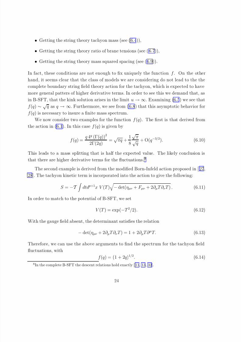
http://slidepdf.com/reader/full/0011226 24/32
• Getting the string theory tachyon mass (see (6.4)),
• Getting the string theory ratio of brane tensions (see (6.7)),
• Getting the string theory mass squared spacing (see (6.9)).
In fact, these conditions are not enough to fix uniquely the function f . On the other
hand, it seems clear that the class of models we are considering do not lead to the the
complete boundary string field theory action for the tachyon, which is expected to have
more general patters of higher derivative terms. In order to see this we demand that, as
in B-SFT, that the kink solution arises in the limit u → ∞. Examining (6.5) we see that
f (q) ∼ √q as q → ∞. Furthermore, we see from (6.8) that this asymptotic behavior for
f (q) is necessary to insure a finite mass spectrum.
We now consider two examples for the function f (q). The first is that derived fromthe action in (6.1). In this case f (q) is given by
f (q) =q 4q (Γ(q))2
2Γ(2q)=
√πq +
1
8
√π√q
+ O(q−3/2). (6.10)
This leads to a mass splitting that is half the expected value. The likely conclusion is
that there are higher derivative terms for the fluctuations.8
The second example is derived from the modified Born-Infeld action proposed in [ 27,
28]. The tachyon kinetic term is incorporated into the action to give the following:
S = −T
dtd p+1x V (T )
− det(ηµν + F µν + 2∂ µT ∂ ν T ) . (6.11)
In order to match to the potential of B-SFT, we set
V (T ) = exp(−T 2/2). (6.12)
With the gauge field absent, the determinant satisfies the relation
− det(ηµν + 2∂ µT ∂ ν T ) = 1 + 2∂ µT ∂ µT. (6.13)
Therefore, we can use the above arguments to find the spectrum for the tachyon field
fluctuations, with
f (q) = (1 + 2q)1/2. (6.14)
8In the complete B-SFT the descent relations hold exactly [11, 13, 32].
24
8/14/2019 0011226
http://slidepdf.com/reader/full/0011226 25/32
Strictly speaking, there is no q that is a solution to eq.(6.5) for this f (q). Instead, we
can modify the function to
f ǫ(q) = (1 + 2q)1
2+ǫ , (6.15)
and take the limit ǫ → 0. In this limit, the solution of (6.5) is q = 2/ǫ → ∞, and so the
width of the brane is shrinking to zero size. Choosing the function in (6.15) and taking
the limit, we see that the open string tachyon mass is m2 = −1/2. We also see from (6.9)
that the spacing between mass levels is twice the magnitude of the tachyon mass squared.
However, the tension of the 8-brane as compared to that of the unstable 9-brane is 2√
π
which is less than the actual value of √
2π.
6.2 Gauge fluctuations for the modified Born-Infeld action
In this section we compute the spectrum for the gauge fluctuations on a kink backgroundfor the action in (6.11). Setting T to the kink solution T = ux and expanding the
determinant in (6.11) to second order in F µν , we have
− det(ηµν + F µν + 2∂ µT ∂ ν T ) = (1 + 2u2)
1 − 1
2F µν N νλ F λδN δµ
+ ..., (6.16)
where
N µν = ηµν − 2u2
1 + 2u2δµxδνx . (6.17)
Hence, up to second order in fluctuations we find
−det(ηµν + F µν + 2∂ µT ∂ ν T ) = 1 +
1
2
(1 + 2u2)F µν F µν + F µxF µx . (6.18)
To find the gauge fluctuations about the kink background, we plug (6.18) into (6.11)
and expand to second order, giving
− T
dtd pydx exp(−u2x2/2)(1 + 2u2)1/2
1
4F µν F µν +
1
2(1 + 2u2)F µxF µx
. (6.19)
Following the arguments in section 3, we find that the spectrum has equally spaced levels
with spacing
∆m2 =u2
1 + 2u2=
q
1 + 2q. (6.20)
Therefore, in the limit q→ ∞
, the spacing of the levels is half the expected value.
While not the desired value, we note that the spacing we found is finite. If the Born-
Infeld action was of the usual type, without the tachyon kinetic term, then for a kink
of the form T = ux, the spacing would have been u2 = q. If q → ∞, as is expected in
B-SFT, this would push the spacing to infinity. That it stays finite seems to provide some
support for the form of the action in (6.11).
25
8/14/2019 0011226
http://slidepdf.com/reader/full/0011226 26/32
6.3 Higher codimension branes
We can also consider higher codimension branes. In the models for the bosonic string
tachyon such solutions existed exploiting the fact that the tachyon potential is unbounded
below. Since the tachyon potential for the superstring is positive definite we need a differ-
ent way to avoid Derrick’s no-go result for higher codimension branes. This would seem
to require several tachyon fields and gauge fields. However, Derrick’s theorem assumes a
standard kinetic operator for the scalar fields. If there are higher derivative terms then
higher codimension objects appear to be possible when we have several tachyon fields,
even without exciting the gauge fields.
In order to construct these higher codimension branes, we thus start with more than
one D9 brane. If we have N such branes, then the tachyons transform in the adjoint of
U (N ). For a codimension d brane, the tachyon configuration has the form [1, 33, 34, 13]
T = Γm u xm , (6.21)
where the index m refers to the transverse directions and the Γm are the d dimensional
Dirac matrices. The tachyon configuration in (6.21) is a solution to the equations of
motion for the action
S = −T
dt d p+1x Tre−T 2/2f (∂ µT ∂ µT )
. (6.22)
with f satisfying
2 qd
f ′(q) = f (q), (6.23)
where q = du2. If we use the two derivative action in (2.26), then we see that there is no
solution for d > 2 and that in the limit d → 2, q is pushed out to infinity.
However, including higher derivative terms leads to solutions with finite values of q.
For instance, suppose that we choose f (q) to be
f (q) = (1 + q/d)d. (6.24)
This choice for f (q) leads to a tachyon mass with m2 = −1/2. It has a solution at q = d,
which corresponds to u = 1. Computing the tension of the codimension d brane, we findthat
T 9−d = 2d/22d(2π)d/2T . (6.25)
The total tension of the 9 branes is 2d/2T , which takes into account the multiple unstable
branes or brane-antibrane pairs, depending on whether d is odd or even. Hence the ratio
26
8/14/2019 0011226
http://slidepdf.com/reader/full/0011226 27/32
of tensions to a single IIB 9 brane is
T 9−d
T 9= 2d(4π)d/2 =
4
πd/2
(2π)d. (6.26)
Hence, this choice for f (q) leads to constant descent relations and can basically be thought
of as the extension to the two derivative truncation for lower dimensional branes.
7 Conclusions
We have extended the previously constructed superstring tachyon effective theory [10] to
include gauge fields and fermions. The complete model, assembled from (2.14) and (5.1)
reads
S = −
dtd p+1xK′(T )2
(∂T )2 + 1 +1
4F µν F µν +
i
2ψ Γµ
↔
∂ µ ψ + W (T ) ψψ
, (7.27)
where K′(T ) =√T exp(−T 2/4), W (T ) = T /2, and we work with p = 8 for the unstable
D9 of IIA. This action gives the correct tachyon mass, and correct mass spectrum for the
tachyon, gauge field and fermion field fluctuations around the kink solution representing
a codimension one brane. On the other hand, the descent relation for the tension is not
exactly that of string theory. As we have explained, the above interactions for gauge
fields and fermion fields result in solvable spectra around brane configurations, but any
action for gauge fields or fermions that is equivalent to this action, up to quadratic order
in those fields, will have the same solvability properties and exactly the same spectrum.
This includes, in particular, Born-Infeld actions of the form
S = −
dtd p+1xK′(T )2 −det(ηµν + F µν ) + · · · , (7.28)
where the dots denote tachyon and fermion kinetic terms. In fact, our analysis of actions
with higher derivatives in section 6 shows that solvability is still possible if, following
[27, 28], we include the tachyon kinetic term inside the square root giving
S = − dtd p+1xK′(T )2 −det(ηµν + F µν + 2 ∂ µT ∂ ν T ) + fermions . (7.29)
Details of the solutions and spectra, however, differ from that of (7.27), since the tachyon
background is changed (it is T = ux, with u → ∞). In particular, the level spacing for
the gauge field fluctuations is half the expected one.
27
8/14/2019 0011226
http://slidepdf.com/reader/full/0011226 28/32
For the bosonic string theory tachyon model the two alternative forms of the action
are based on equations (3.13) and (3.18)
S = − dtd p+1x(L′(T ))2 12(∂T )2 + 2T + 2T
1 14F µν F µν , (7.30)
with L′(T ) = 12
√T e exp(−T /4). The first form is Born-Infeld compatible and has finite ℓ
solvable counterparts. The spectrum of gauge fluctuations, however, has a mass spacing
which is twice the expected one. The second form is not Born-Infeld compatible and
does not have finite ℓ solvable counterparts. On the other hand the mass spacing is the
expected one. Note that neither form is compatible with tachyon kinetic terms inside the
Born-Infeld square root, since the prefactor in the tachyon kinetic term does not coincide
with the tachyon potential. It is not completely clear how to decide between these two
possibilities, but it seems reasonable to choose the form with correct mass spacing. Asreviewed in the introduction, both forms have appeared in B-SFT studies.
In section (6.2) we saw that one could construct stable solutions on the worldvolume of
coincident branes representing branes with codimension greater than one without turning
on gauge fields. This was possible because the tachyon field theory model used had
higher derivative terms for the tachyon, and is why such solutions could be found also
in B-SFT [13]. The existence of such solutions, however, is somewhat puzzling as earlier
discussions of configurations on the world volume of coincident D-branes leading to a
lower dimensional stable branes appear to require non-trivial gauge field backgrounds
[1, 33, 34].
The surprising and pleasant features of the original tachyon models [9, 10] were that
simple field theory interactions exactly described a situation where the tachyon could dis-
sappear completely in the stable vacuum and where nontrivial configurations representing
branes existed with a fluctuation spectrum of stringy type. In retrospect, we see that such
properties essentially guaranteed agreement between these models and the two-derivative
truncations of B-SFT formulations of tachyon dynamics. We have seen in this paper that
these pleasant features nicely extend to models including the interactions of the tachyon
with gauge and fermion fields.
Acknowledgments: J.A.M. would like to thank the CTP at MIT and the theory group
at Harvard for hospitality during the course of this work. We are grateful to Jeffrey
Goldstone for discussions on fermion localization on kinks. We also wish to thank Igor
28
8/14/2019 0011226
http://slidepdf.com/reader/full/0011226 29/32
Klebanov and Leonardo Rastelli for their comments on gauge invariance in B-SFT. Finally,
we would like to thank Ashoke Sen for many useful remarks and discussions. This work
was supported in part by DOE contract #DE-FC02-94ER40818.
References
[1] A. Sen, “Descent relations among bosonic D-branes,” Int. J. Mod. Phys. A14, 4061
(1999) [hep-th/9902105]; “Stable non-BPS bound states of BPS D-branes,” JHEP
9808, 010 (1998) [hep-th/9805019]; “Tachyon condensation on the brane antibrane
system,” JHEP 9808, 012 (1998) [hep-th/9805170]; “SO(32) spinors of type I and
other solitons on brane-antibrane pair,” JHEP 9809, 023 (1998) [hep-th/9808141].
[2] E. Witten, “Noncommutative Geometry And String Field Theory,” Nucl. Phys.
B268, 253 (1986).
[3] N. Berkovits, “Super-Poincare Invariant Superstring Field Theory,” Nucl. Phys.
B450 (1995) 90, [hep-th/9503099].
[4] V. A. Kostelecky and S. Samuel, “On A Nonperturbative Vacuum For The Open
Bosonic String,” Nucl. Phys. B336, 263 (1990);
A. Sen and B. Zwiebach, “Tachyon condensation in string field theory,” JHEP 0003,
002 (2000) [hep-th/9912249].
W. Taylor, “D-brane effective field theory from string field theory”, hep-th/0001201.
N. Moeller and W. Taylor, “Level truncation and the tachyon in open bosonic string
field theory”, hep-th/0002237.
J.A. Harvey and P. Kraus, “D-Branes as unstable lumps in bosonic open string field
theory”, hep-th/0002117.
R. de Mello Koch, A. Jevicki, M. Mihailescu and R. Tatar, “Lumps and p-branes in
open string field theory”, hep-th/0003031.
N. Moeller, A. Sen and B. Zwiebach, “D-branes as tachyon lumps in string field the-
ory,” hep-th/0005036.
R. de Mello Koch and J. P. Rodrigues, “Lumps in level truncated open string field
theory,” hep-th/0008053.
N. Moeller, “Codimension two lump solutions in string field theory and tachyonic
theories,” hep-th/0008101.
29
8/14/2019 0011226
http://slidepdf.com/reader/full/0011226 30/32
A. Sen and B. Zwiebach, “Large marginal deformations in string field theory,” hep-
th/0007153.
W. Taylor, “Mass generation from tachyon condensation for vector fields on D-
branes,” hep-th/0008033.
[5] N. Berkovits, “The Tachyon Potential in Open Neveu-Schwarz String Field Theory,”
[hep-th/0001084];
N. Berkovits, A. Sen and B. Zwiebach, “Tachyon condensation in superstring field
theory”, hep-th/0002211;
P. De Smet and J. Raeymaekers, “Level four approximation to the tachyon potential
in superstring field theory”, hep-th/0003220;
A. Iqbal and A. Naqvi, “Tachyon condensation on a non-BPS D-brane,” hep-
th/0004015; “On marginal deformations in superstring field theory,” hep-th/0008127.[6] A. Sen, “Universality of the tachyon potential,” JHEP 9912, 027 (1999) [hep-
th/9911116];
L. Rastelli and B. Zwiebach, “Tachyon potentials, star products and universality,”
hep-th/0006240.
V. A. Kostelecky and R. Potting, “Analytical construction of a nonperturbative vac-
uum for the open bosonic string,” hep-th/0008252.
H. Hata and S. Shinohara, “BRST invariance of the non-perturbative vacuum in
bosonic open string field theory,” hep-th/0009105.
B. Zwiebach, “Trimming the tachyon string field with SU(1,1),” hep-th/0010190.
[7] E. Witten, “On background independent open string field theory”, Phys. Rev. D46,
5467 (1992) [hep-th/9208027];
E. Witten, “Some computations in background independent off-shell string theory”,
Phys. Rev. D47, 3405 (1993) [hep-th/9210065];
K. Li and E. Witten, “Role of short distance behavior in off-shell open string field
theory”, Phys. Rev. D48, 853 (1993) [hep-th/9303067].
[8] S.L. Shatashvili, “Comment on the background independent open string theory”,
Phys. Lett. B311, 83 (1993) [hep-th/9303143]; “On the problems with background
independence in string theory”, hep-th/9311177.
[9] J.A. Minahan and B. Zwiebach, “Field theory models for tachyon and gauge field
string dynamics”, JHEP 0009, 029 (2000) [hep-th/0008231].
30

8/14/2019 0011226
http://slidepdf.com/reader/full/0011226 31/32
[10] J. A. Minahan and B. Zwiebach, “Effective tachyon dynamics in superstring theory,”
hep-th/0009246.
[11] A.A. Gerasimov and S.L. Shatashvili, “On exact tachyon potential in open string
field theory”, hep-th/0009103.
[12] D. Kutasov, M. Marino and G. Moore, “Some exact results on tachyon condensation
in string field theory”, hep-th/0009148.
[13] D. Kutasov, M. Marino and G. Moore, “Remarks on tachyon condensation in super-
string field theory,” hep-th/0010108.
[14] D. Ghoshal and A. Sen, “Normalization of the background independent open string
field theory action”, hep-th/0009191.
[15] B. Zwiebach, “A solvable toy model for tachyon condensation in string field theory”,
CTP-MIT-3018, hep-th/0008227.
[16] F. Cooper, A. Khare and U. Sukhatme, “Supersymmetry and quantum mechanics,”
Phys. Rept. 251, 267 (1995) [hep-th/9405029].
[17] J. Feinberg, “On kinks in the Gross-Neveu model,” Phys. Rev. D51, 4503 (1995)
[hep-th/9408120];
J. Feinberg and A. Zee, “Dynamical Generation of Extended Objects in a 1+1 Dimen-
sional Chiral Field Theory: Non-Perturbative Dirac Operator Resolvent Analysis,”Phys. Rev. D56, 5050 (1997) [cond-mat/9603173].
[18] J. A. Harvey and P. Kraus, “D-branes as unstable lumps in bosonic open string field
theory,” JHEP 0004, 012 (2000) [hep-th/0002117].
[19] L. Cornalba, “Tachyon condensation in large magnetic fields with background inde-
pendent string field theory,” hep-th/0010021.
[20] K. Okuyama, “Noncommutative tachyon from background independent open string
field theory,” hep-th/0010028.
[21] O. Andreev, “Some computations of partition functions and tachyon potentials in
background independent off-shell string theory,” hep-th/0010218.
[22] A. A. Gerasimov and S. L. Shatashvili, “Stringy Higgs Mechanism and the Fate of
Open Strings,” hep-th/0011009.
31
8/14/2019 0011226
http://slidepdf.com/reader/full/0011226 32/32
[23] A.A. Tseytlin, “Sigma model approach to string theory effective actions with
tachyons,” hep-th/0011033.
[24] A. Sen, “Supersymmetric world-volume action for non-BPS D-branes,” JHEP9910
,008 (1999) [hep-th/9909062].
[25] P. Yi, “Membranes from five-branes and fundamental strings from Dp branes,” Nucl.
Phys. B550, 214 (1999) [hep-th/9901159].
[26] O. Bergman, K. Hori and P. Yi, “Confinement on the brane,” Nucl. Phys. B580,
289 (2000) [hep-th/0002223].
[27] M. R. Garousi, “Tachyon couplings on non-BPS D-branes and Dirac-Born-Infeld
action,” Nucl. Phys. B584, 284 (2000) [hep-th/0003122].
[28] E. A. Bergshoeff, M. de Roo, T. C. de Wit, E. Eyras and S. Panda, “T-duality and
actions for non-BPS D-branes,” JHEP 0005, 009 (2000) [hep-th/0003221].
[29] W. Siegel and B. Zwiebach, “Gauge string fields,” Nucl. Phys. B263, 105 (1986).
[30] R. Jackiw and C. Rebbi, “Solitons With Fermion Number 1/2,” Phys. Rev. D13,
3398 (1976); C. Callias, “Index Theorems On Open Spaces,” Commun. Math. Phys.
62, 213 (1978); J. Goldstone and F. Wilczek, “Fractional Quantum Numbers On
Solitons,” Phys. Rev. Lett. 47, 986 (1981).
[31] Ashoke Sen, private communication.
[32] S. Moriyama and S. Nakamura, “Descent relation of tachyon condensation from
boundary string field theory,” hep-th/0011002.
[33] E. Witten, “D-branes and K-theory,” JHEP 9812, 019 (1998) [hep-th/9810188].
[34] P. Horava, “Type IIA D-branes, K-theory, and matrix theory,” Adv. Theor. Math.
Phys. 2, 1373 (1999) [hep-th/9812135].
32