0,) - its - boston college · and renato e. mirollo 3 ~department of mathematics, boston...

Physica D 36 (198q) 23-50 North-Holland, Amsterdam

COLLECF[VE DYNAMICS OF COUPLED OSCILLATORS WITH RANDOM PINNING

Steven H. STROGATZ t,2, Charles M. MARCUS 2, Robert M. WESTERVELT 2 and Renato E. MIROLLO 3 ~Department of Mathematics, Boston University, Boston, MA 02215, USA ZDivision of Applied Sciences and Department of Physics, Harvard University, Cambridge, MA 02138, USA JDepartment of Mathematics, Boston College, Chestnut Hill, MA 02167, USA

Received 11 November 1988 Revised manuscript received 2 February 1989 Communicated by A.T. Winfree

We analyze a large system of nonlinear oscillators with random pinning, mean-field coupling and external drive. For small coupling and drive strength, the system evolves to an incoherent pinned state, with all the oscillators stuck at random phases. As the coupling or drive strength is increased beyond a depinning threshold, the steady-state solution switches to a coherent moving state, with all the oscillators moving nearly in phase. This depinning transition is discontinuous and hysteretic. We also show analytically that there is a delayed onset of coherence in response to a sudden superthreshold drive. The time delay increases as the threshold is approached from above. The discontinuous, hysteretic transition and the delayed onset of coherence are directly attributable to the form of the coupling, which is periodic in the phase difference between oscillators.

The system studied here provides a simple model of charge-density wave transport in certain quasi-one-dimensional metals and semiconductors in the regime where phase-slip is important; however this paper ;~ intended r~rimarily as a study of a model system with analytically tractable cdlective dynamics.

1. Introduction

Large systems of coupled nonlinear oscillators arise in many scientific contexts. They have beeu used to model cooperative dynamical systems in physics, chemistry, and biology, including charge- density waves [13, 15, 19, 40], oscillating chemical reactions [23, 44], and networks of oscillating nerve and heart cells [43, 44]. Coupled oscillators are also of great theoretical interest, as they provide tractable models for studies of nonlinear dynamics in systems with many degrees of freedom [1, 2, 4-9, 11-13, 22- 25, 28, 30-40, 42-46].

1.1. Model

In tiffs paper we analyze the following system of coupled oscillators in the infirfite-N limit:

0,) K N

+ ~ E s i n ( 0 j - 8 , ) , i = I , . . . , N , (1.1) j=l

where 0 i is the phase of the i th oscillator, E, b, K >__ 0 are fixed and the ai are independent random variables uniformly distributed on [0, 2~r]. The many-body system (1.1) provides a model of charge-density wave transport in certain quasi- one-dimensional metals and semiconductors, as discussed in section 1.5 and in [40]. Therefore we shall adopt some of the language used in the charge-density wave literature, giving definitions where appropriate.

The phases 0 i in (1.1) can be visual~ed as a swarm of points moving along the unit circle. The points move without inertia in response to three competing forces. The pinning term b s i n ( ~ - 0 i ) tends to make 0~ stick at the random angle ~.

rangement of the phases 0~. This pinning term is opposed by both the applied field E, which tends to drive the phases at a constant angu'~ar velocity and thus favors moving solutions; and by the co~.pling term ( K/N)Ej sin ( S# - 0~), which tends to make #~ = #j and thus favors ordered solutions. The ratios K/b and E/b determine whether the

0167-2799/89/$03.50 © Elsevier Science Publishers B.V. (North-Holland Physics Publishing Division)

24 S.H. Strogatz et al./ Collective dynamics of coupled oscillators

steady-state solutions of (I.1) are ordered or disordered, static or moving. Without loss of generality we normalize (1.1) by setting b = 1.

Roughly speaking one expects the following steady-state behavior of (1.1): for small E and K the pinning term dominates and the oscillators become pinned at random phases. As E increases with K fixed, the pinned state loses stability at some depinning threshold E - Er (K) and the system evolves to a steady-state moving solution.

Our goal is to characterize the steady-sta,,es and bifurcations of (1.1) as E and K are varied. In particular we will show that the depinning transition is discontinuous: the steady-state velocity of the moving solution jumps up discontinuously from zero at the depinning threshold. Furthermore the transition is hysteretic: if E is decreased, the moving solution does not re-pin until E falls below a separate pinning threshold Er. Similar hysteretic and discontinuous transitions are seen experimentally in certain charge-density wave systems, as discussed in section 1.5.

1.2. Organization of the paper

In section 1.3 we outline our strategy for study- ~ag (1.1) analytically. The main idea is due to Kuramoto [22, 23, 25] and involves a dynamical version of self-consistent mean-field theory. Sec- tion 1.4 introduces the main phenomena exhibited by the model: switching, hysteresis, and delay. In section 1.5 we explah: how the dynamical system (1.1) can be used to model charge-density wave transport in "switching samples." This section is introductory and assumes no prior knowledge about charge-density waves.

S~fions 2-5 concern the mathhematScaA anaAysis of (1.1). In section 2 we obtain all the static equilibrium solutions and analyze their bifurcations as the parameters g and K are varied. In section 3 we use variational methods to calculate the depinning threshold Er, above which the pinned state loses stability and the system jumps to a moving solution.

Section 4 presents an analysis of d e steady-state moving solutions. By seeking travelling-wave solutions of a form suggested by symmetry arguments, we reduce an intinite-dimensional problem to a boundary value problem for a single ordinary differential equation. Perturbation theory is used to obtain formal asymptotic solutions of this differential equation in two re~mes: the high field limit E >> 1 and the large coupling limit K >> 1. Numerical simulations indicate that the moving solution disappears at a pinning threshold El,; we argue that this disappearance occurs when a stable limit cycle corresponding to the moving solution coalesces with an unstable limit cycle.

Section 5 presents numerical and analytical results about delayed depinning in response to a sudden superthreshold drive. We derive an evolution equation for the phase coherence and use it to explain our numerical results.

Section 6 offers concluding remarks. We compare our work with previous studies and indicate some directions for future research.

In the appendix we present the details of the perturbation calculations needed in section 4.

1.3. Infinite-range coupling

A good starting point for analyzing a new many-body system is to assume that the coupling is infinite-range. This assumption usually simpfi- ties the analysis while preserving many of the qualitative features found in models with nearest- neighbor or other kinds of short-range coupling. The infinite-range model (1.1) with b = 1 is

K N E sm(0j-0 ), (1.2)

j - - I

where the factor 1/N n o r m a l ~ the coupling term. Because the sum extends over all j, (1.2) can be conveniently rewritten in terms of a mean-field

S.H. Strogatz et ai./ Collective dynamics of coupled oscillators 25

Fig. 1. The order parameter re it, as defined by (1.3). The radius r characterizes the coherence of the phases 0j and the angle 1/' characterizes the average phase. The collective velocity v is defined as v ffi ~.

In this paper we use this self-consistency argument to analyze the mean-field model (1.4) in the limit N ~ oo. The continuous analogue of (1.4) as N - ~ o o is

e + sin ( . - 0.) +

a ~ [O,2~r], (1.5)

where the order parameter is now defined as

quantity

1 N rei~ = ~ Z ei°j (1.3)

j - 1

to give

E + sin

+rr sin( - 0,), i -- 1 , . . . , N. (1.4)

The quantity re i~' provides an order parameter for the system [23, 25, 28, 40]. As shown in fig. 1, the magnitude r of the order parameter characterizes the arnotmt of order or coherence in the configuration of the 0./, and ~p defines the average phase. The quantity v = ~ measures the average

velocity of the system. At first glance (1.4) appears to be an uncoupled

set of equations:/~i depends explicitly on 0i, a i, E, Kr and ~k, but not on the other 0./. Of course 0i is coupled to all the other Oj, but only through the mean-field quantities r and ~k defined by (1.3). This observation led Kuramoto [22, 23, 95] to the following insight (in a different but related con- text): For finite N, one expects the coherence r and the average velocity v to vary h~ time. How- ~,,~r f , r 1.r~. ~ these v~6at_ions should decrease as O(N-~/2). Hence to find the steady-state solutions of systems like (1.4) in the large N lhnit, one can impose a fixed r and v, solve (1.4) for all the a~(t), and then aemand that the resulting solutions 0~ be consistent with (1.3) at all times. This requirement of self-consistency determines r and v and thus solves the problem.

2'I5

rei~= ~-~--~ foei°,dot. (1.6)

Note that a re-indexing has taken place between (1.4) and (1.5): because the equation of motion (1.4) depends on i only through a i, we can re-label each # in (1.5) by its associated a. This assumes that all oscillators with the same a eventually move identically, regardless of their initial condi- t ions- this is certainly the case in our computer simulations.

1.4. Switching, hysteresis, and delayed onset of coherence

Eq. (1.5) can exhibit interesting dynamics because of its third term Krsin(~p-0~), which represents a collective force that pulls each 0, towards the population average phase ~k. The collective force has an effective strength Kr that is proportional to the coherence r of the whole population. Thus an incoherent population exerts no force on any of its members. On the other hand, once coherence starts to develop, it can set off a positive feedback process: as r increases, the effective coupling Kr increases, thus tending to bl'ing the phases closer together towards ~p, which makes r even larger, and so on. Whether thi~ process becomes self-sustaining depends on the parameters K and E and on the initial conditions. For example, when E = 0 the static pinned configuration 0, = a always solves (1.5): it has r = 0 so the collective pull vanishes, and the p i r~ng forces s i n ( a - e,) are also zero. But is this state stable? Clearly for K large enough the system is prone to

26 S.H. Strogatz et al./ Collective @namics of coupled oscillators

0 . 8 '

0.4

0.0 0.4

1.0

0.5.

,J

..... I' 017 1 '.o Ep E T

1' i,

i

I

Ep

0.0 0.4 0'.7 ET 110.

E

2 . 0 -

1 .5 -

Kc 7 1.0

0.5

0.0

moving . . . . . n : i ill" . . . . . . . .... "-O.o.o.o..

" ..... ".............. ~""ET pinned E.~"..... \

, ,

1.0 0.2 0.4 0.6 0.8 1.0 1.2 i

1.4

Fig. 3. Stability diagram for steady-state solutions of (1.2): solid line, depinning threshold E r = (1 - K2/4) 1/2 determined analyt!,.ally in section 3; dashed line, pinning threshold Er obtained by numerical integration of (1.2) for N = 300 phases.

Fig. 2. Switching and hysteresis between pinned and moving solutions of (1.2). The velocity v and coherence r of the steady-state solutions of (1.2) are plotted against the applied field E. The data were obtained for N = 300 phases by numerical integration of (1.2) with K = 1. As E exceeds the depinning threshold E T the system switches discontinuously from the incoherent pinned state (r = 0, v = 0) to the coherent moving state (r > 0, v > 0). As E is decreased the system switches back to the pimaed state at a separate pinning threshold Ep Because Ep < ET, a hysteretic region is formed.

the feedback process discussed above; it turns out that KT = 2 is the threshold above which stability is lost (section 2.1) and the system jumps into a coherent configuration with r = 1.

We now present the results of numerical experi- ments which illustrate some of the behavior of (1.4) in the large N limit. For any initial conditions the hafinite-N syste~n always evolves to a steady-state solution for which the average veloc- Ry v and the coherence r are both time-independent. Fig. 2 plots the steady-state velocity and coherence of the system (1.4) against the applied field ~ fnr the case of N = 300 os~d!ators and

coupling strength K = 1. For small E the system is pinned (v = 0) and incoherent (r = 0). When E exceeds the depinning threshold Er, the velocity jumps up disconthauously, a phenomenon we call switching by analogy to the switching seen in ~.he current-voltage characteristics of some charge-

density wave systems [10, 15-21, 29, 41, 47]. With further increase in E, the velocity increases nearly linearly. If E is then decreased, the velocity decreases and then switches discontinuously to zero at the separate pinning threshold E = Er as shown in fig. 2(a). Fig. 2(b) shows that the coherence r of these solutions also exhibits hysteresis with discontinuous jumps at E r and Er.

The thresholds Er and Ep depend on the cou- plh~g K, as shown by the bifurcation diagram plotted in fig. 3. The depinning threshold ET(K) is found analytically in section 3:

= 4 ' K _ < 2 ,

0, K > 2 .

Note that for K > 2, the system moves for any E > 0. In other words the depinning threshold ,,~,..,;o~,~o ¢ . . . . . m,.,;,~,,.,,1,, ~, . . . . . . . . . 1:.,,.,,.,, 'T'k~ pin

ning threshold Ep shown in fig. 3 was determined numericaUy using the irdtial condition 0 i = 8j V i, j. We have not been able to derive an analytical expression for EI,(K) when E > 0. The thresholds E r ( K ) and Ep(K) in fig. 3 bound a hysteretic region where both pinned and moving solutions

S.H. S=rogatz et aL / Collective @namics of coupled oscillators 27

6.28'

0.00 0.00

o

o en • • e

• ° o

e ° • • o ° o

e0

Q

t j o 41' °

• ° t b O • o ° • • qj • o

• • •

, ; ": :

6 . ~ ,J

O

0 °

0.00 0.00

O • •

e • •

°: ~. • o o ° " ~ •

• e • o o

• ° ° ° o ~ • •

• • ° o

I Q , 0

6.28 o •

0 . 0 0

e o

e0

• •

o o • o o ~ e

• • o

0 • • e

o

o : ° • •

® ° o

• o o ® qu

6.28

t = 1 e e

• o • e

, t o , '°

, o o° °

o e

o

6 . 2 8

t = 2

-et 7

o : •

0 0

6.28

0.00 0.00

628

0.00 ).00

6.28

,Y e

o , t

# /

6 . 2 8

t = 1 5

. J o

o

o

o

o

i

I , ,2 ( I

0 . 0 0 L _

0.00 (~, 6.28 0.00

t = 5

./J 6.28 6.28"

o j , o

o e o

~ e •

o

628

6.28

= 30

0.0~ 0.00 0.00 CI, 6.28 0.00 C~ 6.28

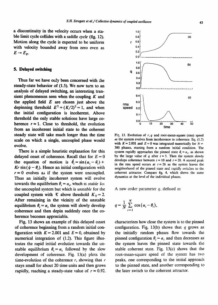
Fig. 4. Delayed onset of coherence for (1.2) when E and K are just above the depixming threshold and the initial state is incoherent. Eq. (1.2) was integrated numerically for N = 300 ph~es, with E = 0 an5 K = 2.06i. For clarity, oniy every fourth phase is shown. The time corresponding to each panel is shown in its upper r i~ t hand comer. Starting from a random initial condition the system first evolves toward the diagonal, corresponding to the pinned state 0 i = % The system slowly leaves the neighborhood of tNs saddle equilibrium, and eventually reaches the coherent final state by t = 30.


are stable; the final state reached depends on initial conditions.

The system (1.4) exhibits a peculiar transient behavior when the system is initially incoherent and when the parameters E and K are chosen just above the depinning threshold: before evolving to the globally attracting coherent state, the system approaches and lingers near a saddle equilibrium corresponding to the pinned state. This results in a delayed onset of coherence.

Fig. 4 shows the evolution of the phases 0o starting from a random initial configuration, with E = 0 and K = 2.001. Note that the panels of fig. 4 are not equally spaced in time. The system first evolves rapidly toward the unstable pinned state 0a "- a, corresponding to the diagonal in each panel of fig. 4. An unstable mode grows slowly and eventually leads to the ripping seen at t = 20. The coherent state is reached by t = 30. A theory of this delayedswitching to the coherent state is presented in section 5.

1.5. Charge-der~ity wave transport

Under certain conditions the behavior of charge- density waves can be modeled by the dynamical system presented in this paper. This section serves as an elementary introduction to charge-density wave transport for readers with no prior exposure ~o the subject. (For reviews see [151 or [191.) This section also discusses the strengths and weak- nesses of our equations as a modal of charge-density wave transport.

A charge-density wave is a collective electronic state found ha certain quasi-one-dimensional metals and semiconductors. In these materials, a uniform distribution of conduction electrons loses stability below a critical temperature, giving rise ~.o a periodic modulation of the charge density with an accompanying periodic distortion of the crystal lattice. Quasi-one-dimensional systems can be realized experimentally in materials which con- duct cu~ent much more readily along one direction than along the other two.

Charge-density wave systems exhibit nonlinear conduction in response to an appfied electric field: when the applied field is weak, the charge-density wave is pinned by impurities o r defects in the lattice and carries no current; above a depinning threshold field E a, the charge-density wave breaks free from the pinning sites and slides through the crystal, carrying current.

Depinning of the charge-density wave can occur either continuously or discontinuously as the electric field is increased. Considerable theoretical attention has been given to the problem of continuous depinning [12-15, 19, 30, 37, 42] which char- aeterizes the bulk of experimental data. On the other hand, systematic studies of discontinuous depinning, known as switching, have begun to appear only recently [10, 15-21, 29, 41, 47]. Switching is seen experimentally as a break in the current-voltage curve as the local electric field crosses E r and the charge-density wave suddenly begins to move and carry current. Hysteresis fre- quently accompanies switching in these systems [18, 47]. That is, after the charge-density wave has depinned, it will not repin until the electric field is reduced well below ET. Switching samples also exhibit a delayed onset of nonlinear conduction in response to a sudden super-threshold applied field [15, 19, 21, 47]. Switching is seen in charge-density wave systems with very strong pinning sites, cre- ated, for example, by radiation-induced defects [10, 16-21, 29, 41].

The charge density p in a one-dh~ensional charge-density wave system can be written as

p ( x , t ) = P o + P c D w C O S ( k X + 8 ( x , t ) ) , (1.7)

where O(x,t) is the phase distortion of the charge-density wave at position x and tLrne t. The charge-density wave has a preferred wavelength 2k = 2~r/k but can be distorted (with some energy cost) to accommodate local impurities or defects in the lattice. When the pinning sites a~c very strong, the charge-density wave can be thought of as consisting of many coupled domains, each associated with one or several strong pinning sites.

S.H. Strogatz et aL / Collective dynamics of coupled oscillators 29

Fig. 5 shows a schematic picture of a charge- density wave as a collection of domains, each with a well-defined phase- tha t is, the phase distortion 0(x, t) is a slowly varying function of x within a domain. Between domains, the amplitude PcDw of the charge-density wave can collapse, allowing the phases of adjacent domains to advance at different rates [16-18, 20]. This phase-slip process relieves the energetically costly phase distortion at the expense of an amplitude collapse betweeq domains.

The effects of pinning, elastic deformation and phase-slip are included in the following simple model [40] for the motion of each domain:

~= E + b sin ( a i - 0,)

+ r E ( Oj - o, ) , J

i= 1,. . . , N. (1.8)

Here 0i is the phase distortion of the i th domain, E is the applied electric field, b is a typical pinning strength, a~ is the preferred random pinning phase for the i'~h domain, and K is the coupling strength between domains, which favors an undistorted wave. The periodic coupling term sin (Oj- Oi) is roughly linear for small phase difference (Oj- Oi). Thus for small pha~e deforma- tions this coupling corresponds to the elastic-coupling assumption used in previous treatments of charge-density wave dynamics [2, 12, 13, 30, 37, 42]. However the sinusoidal coupling also allows phase-slip between domains by giving a restoring force which softens and then reverses as the phase-difference 0 j - 0 i increases.

This paper concerns the dynamics of (1.8) for the case of infinite-range coupling, and shows that tke solutions of (1.8) exlfibit switching, hysteresis, and delayed conduction. In this sense (1.8) provides a simple model of the nonlinear transport processes seen in charge-density wave switcl~ng samples.

However, in addition to the obviously unphysi- cal assumption that all domains are coupled to each other with equal strength, there are several other limitations of (1.8) as a model of charge-

density wave transport: (1) Modellklg phase-slip by a sinusoidal cou-

pling term may capture some of the features of this complicated process, but is certainly not correct in detail. A more realistic model should include the amplitude of the charge-density wave as a dynamical variable. A model of switching in charge-density waves based on amplitude collapse at a single phase-slip center has been analyzed recently [16, 20].

(2) We have made the simplifying assumption that the coupling term in (1.8) is 2~r-periodic in the phase difference 0 i - 0j. This implies that phase-slip between neighboring domains will occur as soon as the phase difference between them exceeds ~r. In real charge-density wave systems a larger phase difference may be built up before a 2~ phase-slip occurs [16, 20]. This has the important physical consequence that many energetically distinct metastable pinned states can exist; such states are observed experimentally [15, 19] but are not present in our model

(3) The pinning strength b should be distributed across domains, rather than constant as we have assumed. This would allow different domains to depin at different apFlied fields, and may lead to multiple switching thresholds, an effect which has been observed experimentally [17, 18].

(4) The role of the "normal electrons"-those conduction electrons which are not condensed into the ch~ge ~ensity wave- has been completely neglected. The normal electrons provide an important parallel conduction path through the material and strongly hffluence the local electric fields felt by the charge-density wave domains.

phase-sUip domain ... . . . , / - region

Fig. 5. Schematic representation of a charge-density wave un- dergoing phase-slip. Strong pinning sites separate the charge- density wave into domains. Between domains the amplitude of the charge-density wave can collapse allowing phase-slip.

30 S.II. Strogatz et at~Collective dynamics of coupled oscillators

2. S ta t i c so lut ions

In this section we consider static equilibrium solutions of the governing equations (1.5). The analysis divides naturally into two cases: E - 0 and E > 0 .

The case E = 0 has been discussed in detail elsewhere [28] and will be reviewed only briefly here. The main result of this section is that there is a j u m p bifurcation in the coherence r when K =

K~ -- 1 .489 a n d K = K T "- 2.

For E > 0, we show that a subcritical branch of static solutions with small r bifurcates along the depinning threshold E r = {i - K 2/4. All of these subcritical solutions are unstable, as can be shown by extending the methods of [28]. In section 2.2, we derive and analyze a self-consistent equation for the.coherence r = r ( E , K ) of these unstable static solutions and show that such solutions exist only if E + Kr _< 1. We argue by contradiction: if static solutions exist for E + Kr > 1, then we obtain the contradiction that the coherence r or some of the phases 0,~ must be complex.

Throughout this section, we emphasize that solutions with r > 0 arise as one-parameter families of configurations parametrized by the average phase ~p. This means that whenever there is one static solution to the equations, there is actually an entire circle of solutions in configuration space. This point is important to keep in mind; although it is obvious for the static case, it helps us to understand the moving solutions studied in later sections-the limit cycles studied there are seen here in degenerate form as circles of fixed points.

Writing the sine functions as complex exponentials and solving (2.1) for the phases 0. yields the equilibrium solution

e i ¢ . ] Kr .t. e i (a -~ , ) eiO., V Kr + e - i ( a - ~ )

= eiq, u + e i~ ( 2 . 2 ) U + e - i v '

where

u = Kr ( 2 . 3 )

and

~, = a - + . ( 2 . 4 )

Thus for each u, there is a one-parameter family of configurations (2.2) parametrized by ~.

2.1.2. Self-consistency equation i'he solution (2.2) must be consistent with the

definition of the order parameter: r e i¢ = (1/2~) fo2~e i°° da. Hence

2"~ • 1/2

Note that the factor e i* cancels from (2.5). Thus q, is arbitrary, reflecting the rotational symmetry in the system. From (2.5) we obtain the self- consistency equation for r:

r = f ( u ) , (2.6)

2.!..~tmit, solutions for E = 0

2.1.1. Explicit form of the solutions For E = 0 the solutions of (1.5) always evolve to

a static equilibrium as t -o oo. These static equilibria satisfy 0,, = 0. Hence

where

2~r • 1/2

o u + e-iv d3,

2"ff

1 f u + cosy = ~ o 1/1 + 2u cos y + U 2 dy. (2.7)

o = oo) + sin ( q , - o,3, a [6,2 r I . (2.1)

The function f (u) may be expressed exactly in terms of elfiptic integrals [28].

S.H. Strogatz et al./ Collective dynamics of coupled oscillators 31

1.0

0.5

o.o

u/K K=K c ..." , .

"-,~...." . . f(u)

0 1 2 U

Fig. 6. Solution of the self-consistency equations (2.6) and (2.7). Solid lines indicate the integral f(u) plotted froth (2.7) together with the line u/K (see tex0. Equilibrium solutions for r occur where f(u) intersects the line u/K. For the values of K shown, three solutions exist (filled circles). Dashed lines show u/K for the bifurcation values K = K¢ and K = K-r = 2.

Fig. 6 shows the graph of f (u) . At fixed K, the corresponding values of r are found at the intersections of the curve r = f ( u ) with the line r = u / K (fig. 6). Note that jump bifurcations occur where the line intersects the curve tangentially, at K = K¢ -- 1.489 and K = Ka- = 2. The resulting curve of of r versus K is plotted in fig. 7.

2.1.3. Stability of the solutions In [28] we prove the following results about

stability: (i) When r = 0, the incoherent pinned solution

0~ = a is globally stable for K < Kc, locally stable for K < 2 and unstable for K > 2. All other solutions with r = 0 are unstable.

(ii) For each u > 0, there is a one-parameter family or "circle" of static soludon~ (2.2)

parametrized by ~p.

1.0'

0.5;

0.0

°'..... "...... °,.

Kc 2 K

Fig. 7. Coherence r of the static equilibrium solutions of (1.5) with E = 0, plotted against the normalized coupling strength K. Solid lines, locally stable equilibria; broken lines, unstable equiEbda. Jump bifurcations occur at g = K¢ and K = 2.

[ \ \ / K c KT

Fig. 8. Schematic bifurcation diagram for equilibrium of (1.5) with E = 0. The coherence r and the average phase ~ of the equilibria are plotted in polar coordinates. The origin r = 0 corresponds to the pinned state 0 a = a, which is locally stable for K < K. r. A circle of saddle equilibria (thin line) and a circle of stable equilibria (thick line) appear at large r when K-- K c. The pinned state 0= = a loses stability at K = K. r when it coalesces with the circle of saddle points. Above K.r the only attractor is the circle of stable points with large coherence

(iii)

(iv)

For u > uc = 1.100, the critical circle is locally stable to perturbations in all d.~xections transverse to the circle. For u < u c, the critical circle consists of saddle points which are unstable in precisely one direction. For all u, the critical points are neutrally sta~-'e to motion along the circle in the ~ direction. The circle of saddles coalesces ~ t h the circle

of stable points at K = K c. As K --, K x = 2, u ~ 0, the saddle configurations for different ~k become more and more alike, and the " 'radius" of the circle shrinks. At K = K T a saddle circle coalesces with the incoherent

pinned state.

2.1.4. Schematic bifurcation diagram Fig. 8 illustrates the transitions discussed above.

The diagram is familiar from the Landau theory of first-order phase transitions or the theory of subcritical Hopf bifurcations. For each equilibrium configuration 0~ given by (2.2), the average phase

is plotted as the polar angle, and the coherence r as the radius. A circle of stable points ~4th large r coalesces with a circle of unstable points at K = K¢, and both are ~ a t e d for K < K c. A small circle of unstable points coalesces ~fith the stable r - - -0 configuration at K = KT, rendering it

unstable for K > KT. Fig. 8 is very schematic because each point

actually represents a configuration 0,, a ~ [0, 2o], and therefore belongs to an infinite-dhmensional


function space, not a two-dimensional space. However, the picture is qualitatively faithful: as shown by (2.2) there is a two-parameter family of equilibria for (2.1), parametrized by the average phase ff and by u = Kr; the topological aspects of the bifurcation are captured correctly by our two- dimensional representation.

Solvhg (2.8) with complex exponentials we obtain

eie,, -._ g + e - i n a ~ [O,2~r],

(2.12)

2.2. Static solutions for E > 0

In this section we compute the shape and coherence of the static configurations for E > 0, and show that they exist only if E + Kr < 1.

where u = Kr.

2.2.2. Existence conditions Eq. (2.12) must be consistevt with (2.11) and

with

2.2.1. Explicit form of the solutions The static solutions now satisfy the equation

2'IT

1 of ei0o r = ~-~ da, r > O. (2.13)

0 = e + s i . ( ~ - 0 o )

+Krsin(~-O,), a ~ [0,2~r]. (2.8)

For r = 0, there are two serf-consistent continuous solutions of (2.8):

0 6 = a + sin -x E (2.9)

and

In particular r must be real. Also we require that 0,, be real for all a.

We show now that these reality constraints are satisfied if and only if u + E _< 1, where u, E > 0. First we rewrite (2.12) in a simpler form. We define p and a by

p e i° --/,/-{- e in, p( g, ~) >__ 0; a( u, if) E [0, 2,1~ I. (2.14)

0~ = a +~r + s in -1E (2.10)

wkere sin- 1 E ~ [ -~ t /2 , ~r/2]. The stability of the solution (2.9) will be

analyzed in section 3, where it is shown that (2.9) is locally stable if and only if E < E T ( K ) = (1 -- / (2/ '4) 1/2. The same analysis shows that (2.10) is ahvays unstable.

For r > 0, there is one-parameter family of solutions of (2.8) for fixed E and K, parametrized by the average phase q~. Without loss of generality, we restrict our attention from now on to solutions with

In terms of p and a, (2.12) becomes

eW. = p C - i n

E + _ E ) 2 . (2.15)

Because we want (2.15) to branch from the stable solution for E = 0, we take the solution (2.15) in which the square root is added to i E/p . Then making the change of variables

~b=0. (2.11)

(To obtain all other solutions, replace #,, and a by 0 6 - ~p and a - ~p respectively.)

sin × = E / O ,

cOS X = 1 - (2.16)

S.H. Strogatz et al. / Collective dynamics of coupled oscillators 33

we obtain e i°o = eiOe ix or

9~ = o + x, a E [0,2~rl. (2.17)

Since a(u,a) and 0, are real for all a, then X = x( E, p( u, a)) must also be real for all a. From (2.16) this condition reduces to

E ~ minp(u~ a) a

= I1 - ul. (2.18)

From (2.12) and (2.13) the self-consistency equation for r is

2= eial 2 E2 1 iE + ¢lu + - r = ~-ff fo u + e-'~ da. (2.19)

The integral (2.19) splits into two pieces. The first piece is

where the star denotes complex conjugation. Thus the integral of g is real:

2'R

fo g(a) da

'IT

= of [g(a) + g ( - a ) l da

'IT

= fo [g(a) + g*(a)l da

= Re g ( a ) d a . (2.23) 0

Combining (2.20) and (2.23) we conclude that

u < 1 (2.24)

2q$

I f ° ie 2~r u + e - i ' '

2'R

B u ' ~ u

= u 2 ~ Izl=l

da

e i " d a

-1 -F e ia

dz g + U - 1

0, u < l , = iE/2u, u = l ,

iE/u , u> 1. (2.20)

The second piece of the hategral (2.19) is real. To see this, let

f g ( a ) = ¢ iu + ei°l z - E 2

u + e -i~ " (2.21)

Because of (2.18) the n,amerator in (2.21) is real for all a. Therefore

is required for the integral in (2.19) to be real. Now (2.18) impfies the stronger i n e q u i t y E < 1 - u or

:., + E < 1. (2.25)

The upshot is that e ~difion (2.25) is necessary and su~cient for tht ~rdstence of static ~olutions for E > 0. (For E = 9, the argument fa i l s -as it m u s t - because the ~-.tegral in (2.20) vanishes.)

2.2.3. Self-consistency equation ]in this section we derive the self-consistency

equation for the coherence r of the static solutions (2.12). By expanding this equation in powers of u = Kr we show that these solutions branch off from the r = 0 pinned solution zJong the curve E2+ K z/4 = 1. It is also shown that this branch is suberitical in the sense that it e×;~sts only for E below threshold ET, where

= v (2.22)

34 S.H. Strogatz et aL / Collective @namics of coupled oscillators

The self-consistency equation is

U

2qT 1 iE + ¢IU + e i*l 2 -

= ~ - of u + e -I°

E 2 d a

2~

1 of ¢a - B' + 2,¢os. +,~ = ~"~ l + 2 u c o s a + u 2

× ( u + cos a) da , (2.26)

where the imaginary part of the integral vanishes as in (2.20) because we are assuming that u + E < I .

Note that u = 0 solves (2.26) for all E, K > 0. To find when solutions with small u > 0 b/fureate from this trivial solution, we expand (2.26) in powers of u << 1. After evaluating the resulting integrals we obtain

u U I U 2 1 + 2E 2 + ~(u4 ) = 2¢1 - e ~ ~1 + T (1 - e ~ ) '-

(2.27)

2.2.4. Static configurations for 0 < r << 1 As E- -~E T, a branch of static subcritical

solutions with small positive r approaches the incoherent (r = 0) solution 0a = a + sin - t E. In fact, an entire circle of subcritical solutions parametrized by ~k coalesces with the incoherent state at E - E T. In this section we calculate the shape of those subcritical solutions to leading order as r-- , 0. As before, we restrict attention to the case ~k = 0 without loss of generality. From (2.17) we have 0a = a + X. We first find a to dT(u) as follows. Eq. (2.14) implies

ei,~__ u + e ia [ u+ eia[

- - ~ u + e i a

U + e - i a

= e-(1 - i ~ sin. + o(.~)) = e i - e - i . ~ o + 0(u2) , (2.31)

SO

o = ~ - u s t n . + ~ ( u 2 ) . (2.32)

Thus non-trivial solufious branch from u = 0 Mong

the c,:~'ve K = 2¢1--=E 2 . For fixed E, let

K T = 2¢1 - E 2 . (2.28)

As K ~ g r from below, the static solutions satisfy

KT U 2 1 + 2E 2 --g- = 1 + T (1 + E2) z + dT(u4)' (2.29)

which "--~" - - LtUpU~,,,~ t h e - - - ~ - - ' : __1 ~__1. _ .__ ~ U U g ; l l t U ~ U~LI~V'iUI-

r ~ (1 + 2E 2

Note that the term in brackets tends to zero (but very slowly) as E ~ 1-.

To find X to 0(u) we recall

sin X = E / p

-- E / t / 1 + 2ucos a + ,.2

= E(1 - ucos a) -e 0 (u2 ) , (2.33)

which can be inverted to yield

uE cos a x = ~ m - ~ E V ~ - E 2 + ~ ( u 2 ) . (2.34)

Hence

0 , = o + X

[ Ecoset ] = ~ + , m - x e - , ~m~+ S_--e~ +~(,=).

(2.35)

S.H. Strogatz etaL/ Collective dynamics of coupled oscillators 35

It is significant that the leading order corrections lie in the subspace of configurations spanned by {sin a, cos a }; as will be seen in section 3, these are precisely the modes which lose stability at the depinning threshold E. r.

This potential function H satisfies

~ = 8H 8%' (3.4)

where

3. Depinning threshold E T

In this section we analyze the local stability of the incoherent pinned solution 0. = a + s in t E. We show that this solution is a local ~ lma of the potential function if and only if ~ < E T ( K ) = ¢ 1 - K2/4. We also find that for A'> E r the pinned state is unstable to small peJ mrba- tions of the form 7(a ) = a sin a + b cos a.

In the presence of an applied field E, the $ov- eming equations are

a,. =.e + o.)

+rrsha(~-O,), a ~ [0,2~r], (3.!)

2~

0

There is a solution of these equations which is pinned (0. = 0 V a) and incoherent (r = 0). Such a solution satisfies E + sin ( a - 0 . )= 0 or

0 , ~ = a + s i n - 1 E , a~ [0 ,2~r ] . (3.3)

Note that this solution exists for all IEI -< 1. The configuration (3.3) is a rotated version of the pinned solution 8. = a found earlier for E = 0. To recover the stable solution found when g = 0, we want the branch of the inverse sine that satisfies cos(sha -~ E) >_ O.

We now analyze the local stability of the pinned state (3.3) by diagonMizing the second variation of the system's potential function about that state.

2~ 2'n

mo=)- -E f O°d"- fo

2.n 2¢

4~ .[ cos(Oa-O,)dadfl. (3.5)

Let 0.(~.) denote a small variation about the static solution (3.3):

O.(c) = a + sin -x E + c 7 , , (3.6)

where c << 1 and 7: a ~ % is a perturbation. For fixed 7, H is a function of the single variable e. W e are particularly interested in the second varia- tiea t" given by

a2 ] (3.7)

because it determines the local stab~ty of (3.3). R~al l that the second variation is a quadratic form in rl; if F is positive defimte, i.e., F ( 7 ) > 0 V 7 4: 0, then the configuration (3.3) is a local minimum of H and is therefore locally stable.

To calculate f ' we first substitute (3.6) into (3.5) which yields

H = -E of (~ + sin - 1 E + c~,) da

2~

- fo c o s ( % + sin - 1 E ) d ~

2Ir 2"~

Jo + 4,rr o

(3.s)


Hence transform:

d H d~

255 2"n'

× sin (o1~ + sin -~ E)da 255 2~r

K

× Sin ( fi -- a + o1# -- via) da dfi, (3.9)

and

255

d2Hd, a - f0 r/~cos(,71. + sin - 1 E ) d a

2.~ 255

x cos ( ¢ - . + ,n# - ,no) d . an. (3.10)

To find F we evaluate (3.10) at c = 0. Thus

2,1t

r(n) = ~h - E = f e n . 0

255 255 K

0 o (3.11)

255 255

255 2,~

= of of~iJ/#(eos acos fl + sin a sin fl) da dfl

= of~l.cosada + ~l .s inada

255 12 = of ~a e i " d a

- 4 ~ 2 1 ~ ( - 1 ) 1 2 , (3.13)

where the Fourier transform ~ is defined by

255

(3.14)

The upshot is that (3.11) may be rewritten as

255

F(~) = V/1 - E 2 o f ~ d a - 2~rKl~(-1)l 2

= 2~[¢1 - E2 Ilrfl[ 2 - K [ ~ ( - 1)12], (3.15)

where

The second integral on the fight side of (3.11) may be simplified in two steps. First, when we expand the term (~a_%)2, only the integral involving rl,~a survives- the others integrate to zero. Hence

2~ 2qr

iv" o f 2~ 2~

= -z f fnono=os(~-.)a=aa. o o

(3.12)

255

il~ll2= 2~ ° f ~ : d " " (3.16)

The quadratic form (3.15) can be d/agonalized as follows. We work in the Hflbert space L2(S x) of square integrable functions with the inner product

255

if ~" u = 2--~ ~,p~ da. (3.17) 0

Second, we expand the term c o s ( f l - a ) on the right side of (3.12) and note that the a and integrals separate, conveniently yielding a Fourier

Let

~ = cosa, v, = sina. (3.18)

S.H. Strogatz et al./ Collective dynamics of coupled oscillators 37 Then II/~112= II1,112-- !2 and ~. i, = O. Write ~ in an orthogonal decomposition using/t and I,:

~a Pa i (3.19)

where la" ~1 ± - I" ~1 ± - 0. That is, we express ~ as a linear combination of tt, p, and some function ~1" orthogonal to b o t h / t and 1,.

Then

117112 -- a + + b 2 + I1~11 + (3.20)

and

I ~ ( - 1 ) 1 2

2,r )2 "- ~ ~l, ,cosada +

=

= ( a l b l l ) e + (b l ld l ) e

ae + b z

2 "

2-1 0f Sin ada

(3.21)

Note that at E = E T the unstable subcritical solutions (3.12) coalesce with the incoherent state (3.3), as shown in section 2.2.3.

The present analysis also reveals the instabifity modes. For E > ET, the incoherent state (3.3) is unstable to any perturbation of the form

= a cos a + b sin a, (3.24)

which is a linear combination of eigenfunctions (3.18). To leading order in r, this is precisely the form of the subcritical solutions (2.35) as they approach the r = 0 state (3.3). In terms of Fourier series, the first harmonic of 0~ is unstable, while all higher harmonics are stable. This instability of the first harmonic is strikingly apparent in fig. 4, between t = 5 and t = 20.

4. Moving solutions

Thus (3.15) has been diagon_afized to the form

l r ( n )

= ¢1 - K 2

( 3 . 2 2 )

Eq. (3.22) expresses F as the sum of two for~s: []~-LIIz is positive definite, and the form c o n t a h ~ g a z + b: is positive, zero, or negative depending on the quantity ~ /1- E e - K / 2 . I n particular, F is

ifive definite/f and only if ~/1 - E z _ K / 2 > 0. Aence the incoherent pinned state (3.3) loses stability at the deph~ning threshold given by

K2 E T = 1 4 " (3.23)

In this section w.- analyze the steady-state moving ~olufions of (1.5). In section 4.1 we seek travelling-wave solutions of a certain form motivated by symmetry arguments and the results of computer simulations. This ansatz reduces the original infinite-d~mensional dynamical system to an ordinary differential equation in one variable, subject to three side conditions. Sections 4.2 a~-~d 4.3 use regular perturbation theory to approximate the wave-shape, coherence, and velocity of the s~ab~e moving solution for large E (section 4.2) and large K (section 4.3).

Numerical results indicate that steady-state moving solutions exist if and only if E exceeds the pruning threshold E p ( K ) . Section 4.4 discusses the bifuccafion that occurs at E = Ep. We conj~- ture that the stable mov-'_ag solution, which corre 7 sponds to a stable limit cycle in configuration space, ceases to exist when the stable cycle coalesces with a saddle cycle.

38 S.H. Strogatz et aL / Collective dynamics of coupled oscillators

4.1. Ansatz for moving solutions

The governing equations for the infinite-N system are

sin( - +Krsin(¢/-O,,) , a ~ [0,2~r].

2~

I [ eiOo da r e i ~ =

O( ix + 2~r, t) = O(a, t) + 2~rm,

(4.1a)

(4.1b)

for integer m. (4.1c)

(iv) The moving solution is locally asymptotically stable for E v < E < E a. and globally asymptotically stable for E > ET.

Property (i) above is the key to analyzing (4.1) for moving solutions. A more explicit statement of property (i) is that there is a 2~r-pedodic function ~,: R-- , R such that (4.1) has a solution of the form

O ~ ( t ) = ~ ( t ) + , ( a - ~ ( t ) ) , a ~ [O,2~t]. (4.2)

As always, we assume E, K >_ 0. Numerical integration suggests that for E >

E v ( K ) (4.1) has a unique, locally asymptotically stable moving solution with the following proper- ties:

(i) All the 0~ execute identical motions but shifted in time and phase.

(ii) The coherence r and the collective velocity v = q; axe both independent of time.

(iii) The solution O, has degree m = O:

O(a, t) = 0 ( ~ + 2~r, t ) V a , V t.

Note that the same function ~ appears in the ansatz for each 0,, a ¢ [t3, 2~r]; this is the sense in which all the 0, execute identical motions. A simi- lax ansatz has been used by other authors [13, 30, 371.

Fig. 9 illustrates a heuristic argument for the ansatz (4.2). The first term on the right side of (4.2) brings us into a reference frame moving with the average phase ~(t). In this frame at a fixed time, some 0. axe ahead of ~ and some axe lagging it, depending on the location of their pinning phase a relative to ~k (fig. 9). As time evolves

0((~, t)

2

0

-./L 2

°

..." t= t~

t L ~ . . . . , I

2 2

Fig. 9. Solutions O(~, t) of (4.1) for four equally spaced times, as obtained by numerical integration. The solutions at different times have identical shapes, but differ by a translaSon along the dashed line O = ~. Equivalently, one solution is related to another by a translation in both the O and a directions. This observation mot;"ates the ansatz (4.2).

S.H. Strogatz et aL / Collective @namics of coupled oscillators 39

q~ ( t ) advances uniformly according to

~(~) = o t . (~.3)

Cancelling e i~ and equating the real and imaginary parts of both sides of this equation, we obtain

Meanwhile the position of the leading O. moves like a travelling wave in the a-direction; hence the wave variable a - ~k (t) = a - vt appears as the argument of ~b in (4.2). The function ~ describes the shape of this travelling wave; in particular q~(a) = 0,(t = 0), since ~k = 0 when t -~ 0.

Now we use (4.2) to obtain a differential equation for the function q~. The argument of ~b is the wave variable ~ defined as

¥--- a - ~ ( t )

= a - o r . (4.4)

Differentiating (4.2) with respect to time we obtain

Oo = 4 + , ' (v ) ( -q ; ) = v(1 - * ' ( 7 ) ) , (4.5)

where prime denotes differentiation with respect to ~,. Also

s~( ,~-~o) = ~ m ( . - [ ~ + ,1) = s i n ( v - , ) (4.6)

and

2,ff

r = ~ cos q~(V) dy, (4.8b)

2,ff

0 = of s in~(y )dT , (4.8c)

since r is assumed to be real and non-negative. The conditions (4.8b, c) may be expressed more compactly as r = (cos q~) ,and 0 = (sin ~), where the averaging operator ( . ) is defined by

2,I1"

(f) = ~ ff(a,)dv. 0

The periodicity condition (4.1c) may be rewritten in tern:s of ,~. as ~(y + 2 , r r )=~(y )+ 2~,m. As mentione:l above in property (iii), numerical simulations suggest that the moving solution has degree m = 0; hence we seek solutions satisfyi~g

q~(Y) =q~(V + 2~r) V Y ~ [o,2~1. (4.8d)

K~ s i n ( # - 0~) = r~ s i n ( + - [ # + , 1 ) = - K r s in q~. (4.7)

Hence (4.1a) becomes

v(1 - q ¢ ) = E + sin (y - q~) - K r s ' . ~ , . (4.8a)

The self-consistency condition (4.1b) may be rewritten as foUows:

2,ff

e ie~ d a

2'ff 1

= ~ f ei~ei~(v)d7 • 0

The problem posed by (4.8) is thus: Given E > 0, K >_ 0; find a 2~r-periodic function ~ and two numbers r >_ 0, v > 0 such that ~ solves the differential equation (4.8a) and satisfies the side conditions (cos~) = r and (s in~) =0. This is a boundary value problem with three degrees of g . . . . A,,~m Q n h ~hr~a onnct r~ in t~ 1~','3r ~ m n ] e _ f o r

fixed E and K we can choose values for ~(0), r, mad v. Then we shoot forward to y=2cr by integrating (4.8a) ~dth the chosen kfitial condition 4,(0) and the chosen parameters r and v. This yields a function ~(y) which depends on the chosen ~(0), r and v. If this function satisfies the side conditions (cos~) = r, ( s in~) =0, and ~(2~r) =

40 S.H. Strogatz et al./ Collective @namics of coupled oscillators

~,(0), then (4.8) has been solved. Otherwise we need to choose a different triple (¢(0), r, o) and continue the process.

From this argument it is not at all clear whether there will be any solutions to (4.8). Because we have as many degrees of freedom as we have constraints, there is reason to hope that solutions exist. In the next two sections we present formal asymptotic solutions of (4.8) for the cases E >> 1 and K>> 1.

(After this work was completed, Nancy Kopell pointed out to us that the implicit function theorem can be used to prove the existence of solutions to (4.8) for sutiiciently large E. This argument will be presented elsewhere.)

4.2. Perturbation theory" E >> 1

Numerical integration indicates that for E >> 1 and K = dT(1), there is a stable moving solution to (4.8) with

v - - E , r ~ l and ¢ < < 1 . (4.9)

That is, the high-field moving solution has all the 0,~ nearly aligned with the average phase ~k.

These observations suggest that we seek a for- real solution of (4.8) as a perturbation expansion in powers of

= 1 / E << 1. (4.1o)

Our strategy is to write expansions for r, o, and ~(~,) in powers of c; then we solve the resulting differential equations at each oider of c, and use the conditions (4.8b, c,d) to determine the con- stares of integration and the ~ o r , - n paramel,ers in r and v. This procedure is carried out far enough to reveal the leading order dependence of ~b, r, and v on c and If.

One word about notation: for convenience, we often suppress the dependence on parameters in the expansions for v, r, and ~. The explicit depen-

dences are

v=v(c,K), r = r ( , , K ) , (4.11)

¢ = ¢ ( a , , e , r ) .

Using e = 1 / E we rewrite (4.8a) as

e v ( 1 - ~ ' ) = 1 + e s i n ( T - ~ ) -eKrsinck. (4.12)

As mentioned above, we expect v ~ E and hence ev ~ 1 as e ---> 0. Hence we expand ev as

co = v 0 + co 1 + e202 + . - . (4.13)

with the expectation that v o = 1. The expansions for ~(T) and r are

~ ( T ) - ' ~ o ( T ) + e ~ t ( T ) + e 2 ~ 2 ( T ) + . .- , (4.14)

r = r o + cr 1 + c2r2 + . . . . (4.15)

In the appendix we carry out the analys; o in detail. The results are:

1 1 ¢'(T) = ~ COST + ~--'~(K si~, T + ¼ sinE3,)

1 + ~--~ ( [ ¼ - K 2 ] cosy - ~ If cos2T

-±12 cos 3T) + O(E-4) , (4.16)

r = l 1 1 2 - 4 E - ' ~ + ~ - - E - ~ ( K - ~ ) + d T ( E - S ) , (4.17)

1 1 ~x , ,,r t ,-4) (4.18) = E - + ( K :

Fig. 10 shows that our third-order series solutions agree well with numerical solutions even when E = dT(1). For E >> 1 the series solution is uxux~tmE, ua:m~.ux~ f i t h T ~ e i ' l C ~ ~ ^ l - - ' : . . . . j ~U" U.NdLUJUL 9 CMLIt~..IL

is therefore not shown.

4.3. Perturbation theory: If >> 1

We now consider the strong-c~upling limit K>> 1 with E=O(1) . The techniques are very

S.H. Strogatz et al./ Collective @namics of coupled oscillators 41

0.6

0.4

0.2

0.0

-0.2

-0.4'

-0.6 0

• numerical integration .~ - - , . , . . . ~ "

i i i

~ 2~ 3'

0.3 0.2 0.1 0.0

-0.1 -0.2 -0.3

0

~ - numerical integration theory

i i b

~ 2~ Y

Fig. 10. The data points show the steady-state configuration ¢(~,) obtained by numerical integration of (4.8) for K = 1 and E = 2. The perturbation theory result (4.16) is plotted as the continuous curve; it compares well with the numerical solution, even though E is far from the high-field limit E >> 1 on which the perturbation theory is based.

Fig. 11. The data points show the steady-state configuration @(y) obtained by numerical integration of (4.8) for K = 4 and E = 0.5. The perturbation theory result (4.21) is plotted as the continuous curve; it compares well with the numerical solution, even though K is far from the strong-coupling limit K >> 1 on which the perturbation theory is based.

similar to those of section 4.2, but the analysis is slightly easier; at each order of perturbation theory, the next term in the unknown function ck is generated by differentiation rather than integration of previous terms.

The main results are asymptotic expressions for the configuration ~ ( r ) , the coherence r, and the collective velocity v, expanded in powers of 1/K. We find that for small E the velocity v is proportional to the applied field E. In particular, the depinnmg threshold ET vanishes in this strong- coupling limit K >> 1. The results of sections 2 and 3 prove the stronger result that E T ( K ) = 0 for all K > 2. Fisher [12, 13] also found these results (v 0c E and vanishing E T in the strong- coupling limit) for a closely related mean-fidd

model. In this sect/on, the small parameter c is given by

, .= 1 / K .

The detailed calculations are carried out in the appendix. The results are:

1 1 q,('y) = ~ sin~ + ~-~(Ecos ~' - i sin 2,/)

r = l - ~

1 2] + ~ - ~ ( [ ¼ - E s i n ' y - ( E c o s 2 y

1

4 K ' ~ 4 64 6

(4.21)

(4.22)

o 1 -~ = 1 - ~ + 0 (4.23)

2K 2

Fig. 11 shows that the solution agrees well with numerical results even if K is not large.

Then (4.8a) becomes

1 v(1 - ¢ 9 = E + sin ( r - ¢) - -fr sine.

We seek solutions o: the form

,/, = ¢o+ ~¢~ ÷ . . . ,

r=ro+~r l + . . . ,

O=Oo+¢O1+ . . .

subject to the conditions (4.8b, c, d).

(i,,.2o)

4.4. The pinning threshoM Ep

We now offer some conjectures about the bifurcation at E = Ep(K). First consider the static case when r~ = v, for wmcn"' we ziavc el~olou~ ~ul~- . Fig. 3 indicates that the point E = 0, K = K c lies o:. the phm/ng threshold. As discussed in sectic~v.s 2.1.3 and 2.1.4, for K slightly greater than K c the system has a circle of saddle equilibrium points and a circle of stable equilibrium points in the full space of configurations (fig. 8). These circles are

4 2 S.H. Strogatz et al./ Collective @namics of coupled oscillators

parametr ized by ,:,. A jump bifurcation occurs at

K = K c as the circle of saddle po in t s coalesces

with the circle of stable points. For K < K c the

sinks and saddles have annihilated, leaving the

incoherent pinned configuration O(a)= a as the only attractor. These statements were proven

in [2s]. For K > K c and E = 0 , the circle of saddle

points and the circle of stable points are each neutrally stable to motions along the circle, as discussed in section 2.1.3, For E = 0 +, we conjec- ture that the circle of stable points loses this neutral stability and becomes a stable l imit cycle. The circle of saddle points for E = 0 is expected to become a saddle cycle for E > 1 - Kr, as discussed in section 2.2.2.

Fig. 12 shows these limit cycles and their bifur-

cations in a schematic format analogous to fig. 8.

Each of these cycles in configuration space repre-

sents a moving solution to (4.1). The motion along

the cycles is expected to be uniform, because of

the rotational symmetry in the problem.

Fig. 12 leads us to believe that the pinning threshold Ep(K ) is defined by the condition that the stable cycle and the saddle cycle haoe coalesced. As

E ~ Ep(K) one of the Floquet multipliers (corre-

sponding to perturbations transverse to the stable

cycle and toward the saddle cycle) is expected to

approach zero.

However the velocity along the cycles is not

expected to approach zero as E ~ Ep (K) . Thus

we expect a genuine discontinuity in the velocity v

at E = Ep(K) , as indicated in fig. 2(a). If correct, this discontinuity in v would be of theoretical

interest because it distinguishes the repinning of

this system from that of the hysteretic dc-driven Josephson junct ion and the damped pendulum

driven by a constant torque. Daniel Fisher has

pointed out to us that in these latter systems the

analogue of the velocity tends to zero continuously ~vu~ w~m infinite oenvauves o~ an orders) as ~ Ep, according to

1 v c~ In ( E - Ep ) " (4.24)

! Ep

oo o \ /

I I Es E T

(a)

2.0

Kc/

1.0

0.0 0.0

moving

E; ,E,

0.5 1 .o E

(b)

Fig. 12. (a) Schematic bifurcation diagram for steady-state solutions of (4.1) with E > 0. The coherence r and the average phase if(t) of the solutions are plotted in polar coordinates. The origin corresponds to the pinned state 0,--a + sin-l E, which is locally stable for E < E T. A saddle limit cycle (thin line) and a stable limit cycle (thick line) are born at large r when E-- Ep. Motion along the saddle cycle stops at E = E s, giving rise to a circle of saddle equilibrium points; the stopping threshold E s is defined by the condition E + Kr = I given in (2.25). The circle of saddle points coalesces with the pinned state at E = E T. At this coalescence the r = 0 pinned state becomes unstable. Above E T the only attractor is the stable limit cycle corresponding to the coherent moving solution. (b) Stability diagram as in fig. 3, but with the stopping threshold E s added. The points (K s, Es) on the stopping threshold are defined by the parametric equations E s = 1 - u and K s =

u/r(u); the coherence r(u) was obtained by numerical quadra- ture of the integral in (2.26).

For the Josephson junction, v and E correspond

to the dc-voltage and the applied current, respec-

tively; for the driven pendulum they represent the

average velocity and the applied torque.

The bifurcation which leads to (4.24) has com-

pletely different phase space geometry from that

in our system: t-'he velocity dependence (4.24)

occurs when a stable limit cycle passes near a

saddle point, and motion on the cycle becomes

extremely non-uniform and slow in the neighbor-

hood of that point. We believe that in our system,


a discontinuity in the velocity occurs when a stable limit cycle collides with a saddle cycle (fig. 12). Motion along the cycle is expected to be uniform with velocity bounded away from zero even as E "-* Ep.

5. Delayed switching

Thus far we have only been concerned with ~,he steady-state behavior of (1.5). We now turn to an analysis of delayed switching, an interesting transient phenomenon seen when the coupling K and the applied field E are chosen just above the depinning threshold E 2 + ( / ( /2)2= 1, and when the initial configuration is incoherent. Above threshold the only stable solutions have large coherence r - -1 . Close to threshold, the evolution from an incoherent initial state to the coherent steady state will take much longer than the time scale on whick a single, uncoupled phase would evolve.

There is a simple heuristic explanation for this delayed onset of coherence. Recall that for E = 0 the equation of motion is 0 i = s i n ( ¢ i - 8 ~ ) + Kr s i n ( ~ - 0~). Hence an initial configuration with r = 0 evolves as if the system were uncoupled. Thus an initially incoherent system will evolve towards the equilibrium 0~ = ai, which is stab& fcu ~ the uncoupled system but which is unstable for the coupled system with K above threshold K-r = 2. After remaining in the vicinity of the unstable equilibrium 0 i = a~ the system will slowly develop coherence and then depin suddenly once the coherence becomes appreciable.

Fig. 13 shows an example of this delayed onset of coherence beginning from a random initial configuration with K = 2.001 and E = 0, obtained by numerical integration of (1.2). This figure illustrates the rapid initial evolution towards the unstable equilibrium 0~ = a~ followed by the slow development of coherence. Fig. 13(a) plots the time-evolution of the coherence r, showing that r stays small for about 20 time units and then grows rapidly, reaching a steady-state value of r---0.92.

1.0

0.8

0.6

0.4

0.2

0.0

(a)

0.6

(1.4

• . . . . i . . . . i . . . . t . . . . i . . . . i

rms speed

0.4

0.3

0.2

o.1

o.o o

(c)

lO 20 30 40 50 t ime

Fig. 13. Evolution of r, q and root-mean-square (rms) speed as the system evolves from incoherence to coherence. Eq. (1.2) with K = 2.001 and E = 0 was integrated numerically for N = 300 phases, starting from a random initial condition. The system rapidly approaches the pinned state 0, = a,, as shown by the large value of q after t - -5 . Then the system slowly develops coherence between t -- 10 and t - 20. A second peak in the rms speed occurs at t = 26 as the system leaves the neighborhood of the pinned state and rapidly switche~ to the coherent attractor. Compare fig. 4, which shows the same dynamics at the level of the individual phases.

A new order parameter q, defined as

1 N q = ~ E c ° s ( a i - S i ) ,

i----1

characterizes how close the system is to the pinned configuration. Fig. 13(b) shows that q grows as the initially random phases flow towards the pinned configuration ~i = ai and then decreases as the system leaves the pinned state towards the stable coherent state. Fig. 13(c) shows that the root-mean-square speed of the system has two peaks, one corresponding to the initial approach to the pinned state, and another corresponding to the later switch to the coherent attractor.

10 5 The choice E = 0 used above is special in the sense that the steady-state solution is static, but this does not affect the qualitative features of the delayed switching. Throughout this section we will

concentrate on the case E = 0. The ease E > 0, which is relevant to the delayed switching observed experimentally in some charge-density wave systems [21, 47], will be discussed in a subsequent

paper . In section 5.1, we present data from numerical

simulations characterizing delayed switching for the case E = 0. In particular we study the dependence of the time delay • on the proximity to threshold defined by g = K - K T. Section 5.2 presents an analytical expression for the delay • in terms of ~ and the initial coherence r 0. The results presented in section 5.2 are derived in section 5.3 using regular per turbat ion theory about the unstable equilibrium at 0~ = a~. The a~alysis makes use of the fact that nearly all of the time delay occurs as the system is leaving this unstable equilibrium.

5.1. Switching delay for E = 0: Numerical results

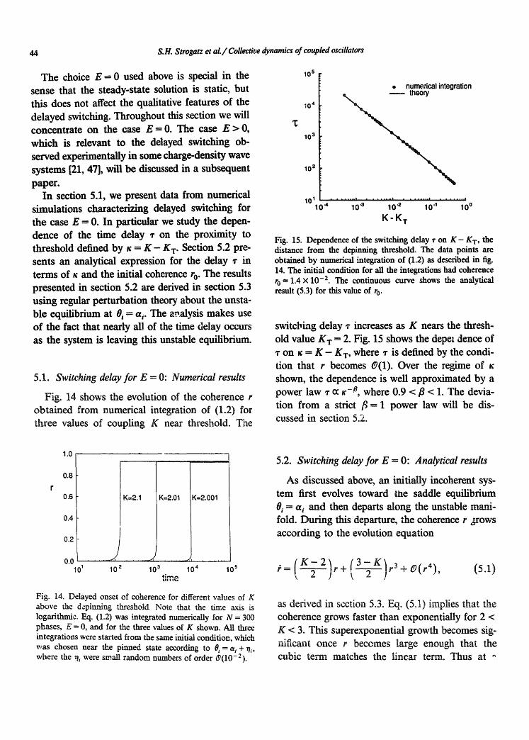
Fig. 14 shows the evolution of the coherence r obtained from numerical integration of (1.2) for three values of coupling K near threshold. The

• numerical integration

10 4

10 3

10 2


l o ' . . . . . . . . 0 "~ . . . . . . . . . . . . . . . . . '0 ~ ......... 10 4 1 10 .2 1 10 0

K - K T

Fig. 15. Dependence of the switching delay ~" on K - g T, the distance from the depinning threshold. The data points are obtained by numerical integration of (1.2) as described in fig. 14. The initial condition for all the integrations had coherence r 0 = 1.4 × 10 -2. The continuous curve shows the analytical result (5.3) for this value of r 0.

switching delay • increases as K nears the threshold value K T --- 2. Fig. 15 shows the depel dence of ~" on ~ = K - K T, where 1" is defined by the condition that r becomes ~(1). Over the regime of shown, the dependence is well approximated by a power law ~- ~ ~-a, where 0.9 </3 < 1. The devia- tion from a strict fl = 1 power law will be discussed in section 5.2.

1.0

0.8

0,6

0.4

0.2

0.0 01 10 2

K=2.1 K=2

. . . . . . ~ . .

103

t l l i I~,,*

K=2.001

10 4 10 s

Fig. 14. Delayed onset of coherence for different values of K above the depinning threshold, Note that the time axis is logarithmic. Eq. (1.2) was integrated numerically for N = 300 phases, E = 0, and for the three values of K shown. All three integrations were started from the same initial condition, which was chosen near the pinned state according to O, = % + ~i, where the ~, were small random numbers of order 0(10-2).

5.2. Switching delay for E = 0: Analytical results

As discussed above, an initially incoherent system first evolves toward me saddle equilibrium 0 i = ai and then departs along the unstable manifold. Dur ing this departure, the coherence r 3rows according to the evolution equation

(5.1)

as derived in section 5.3. Eq. (5.1) implies that the coherence grows faster than exponentially for 2 < K < 3. This superexponential growth becomes significant once r becomes large enough that the cubic term matches the linear term. Thus at ~

$.H. Strogatz et a l . / Collective dynamics of coupled oscillators 45

value of r given by exponentially according to

r 2 _ K - 2 3 - K (5.2)

the system evolves superexponenfially and suddenly switches to the coherent state.

The condition (5.2) provides a natural definition of the time at which switching occurs. If the initial coherence satisfies r0 2 << ( K - 2) / (3 - K) , then the

k

first term on the fight side of (5.1) is initially dominant and the coherence grows according to r ( t ) ~ ro eKt/2. (Here t is measured from the time when the system first reaches the neighborhood of the pinned state.) Then the switching time • is defined by thecondit ion (5.2):

K - 2 3 _ K -- ro2e ~* .

For ~ = K - 2 << 1 this yields the switching delay

1(,) ~" --- -- In - - (5.3) r 2 "

Fig. 15 shows that this theoretical value of the delay agrees well with the values obtained by numerical integration of (1.2). In general (5.3) != expected to hold for K in the range r0 2 << x << 1.

A theory of delayed switching which neglected the cubic term in eq. (5.1) would yield ~" cc ~-# with fl = 1. Although (5.3) is dominated by the 1 / ~ term for r << 1, the important logarithm term affects not only the magnitude of the delay but also its scaling with x, giving an approximate value of fl which is less than one. For the values of K and r 0 used In our numerical integration, both the numerical data and co. (5.3) can be fit by

,~, . ,~, .~. . , ; , , . ,, , . d . . . . . t - _ _ . K-- ~ • , .VV,,, ,~,,~t,, , ly p o w e r l a w "r

= 0.96. This approximate power law was obtained for ~: in the range 10 -4 < ~: < 10 -~.

The cubic term in (5.1) is also important for r 2 > ( K - 2)/(3 - K ), in which ease the cubic term dominates ff, e finear term from the starL In par- titular, at threshold the coherence grows non-

r ( t ) -- (r0 - z - t) -1/2 [for K = KT= 2] (5.4)

before r saturates near 1. Eq. (5.4) shows that the timescale at threshold is O(ro2), which is much longer than ~- in (5.3) for small r 0. On the other hand, (5.4) also shows that the delay before r becomes 0(1) does not diverge as K ~ K r.

5.3. Evolution equation for coherence

We now derive the evolution equation (5.1). This equation describes the growth of coherence for a system evolving along the unstable manifold of the saddle pinned state. In the infinite-N limit the dynamics of the .,h . . . . . " E = 0 are governed by

= s i , - o . ) + . 0o) . (5 .5 )

We must now find a self-consistent solution for u, as before, but with the added compfication that u(t) evolves in time.

In numerical solutions of (5.5) the average phase remains essentially constant as the phases O~

evolve. We make use of this observation by seeking solutions of (5.5) of the form

= + ¢ ( a - u) (5 .6 )

and insist that

throughout the evolution. This ansatz (5.6) is closely related to that used in section 4.1; the difference is that here u depends on time and ~ is th-ne-independent. This ansatz is valid after the system has completed its initial rapid evolution toward the pinned state and has begun to depart very. slowly from the saddle planed state 'along its unstable manifold.

Substituting (5.6) into (5.5) yields

sin(v using, (5.7) O, uU = - _


where y - a - ft. The self-consistency equation for u is

,, = r ( ~ s #,), (5.8)

where the brackets denote the average over one cycle of 7, as in (4.8b).

Two symmetries of (5.7) restrict the form of its solutions: First, (5.7) is invariant under the transformation

y . . .~ o y ,

#,--, -q,

and therefore its solutions must satisfy

4,(,, v) = - , ( , , - v ) . (5.9)

Second, (5.7) is invariant under the transformation

y--+ V +~r,

#,--* ~ + ~r, U---~ - - U

and therefore its solutions must satisfy

~ + , ( . , v ) = , ( - . , , , + ~). (5.1o)

We assume that close to the unstable equifib- rium q~(u, y)=~,, we can express q~-~, as a Fourier series in ~, with small amplitudes ak(U ) which grow as the system leaves the unstable equilibrium and develops coherence. The symmetries (5.9) and (5.10) require that such solutions be o f the form

oO

* ( . , v ) = v - E ~ ( . ) ~ m k v , (5.11)

where the ampfitudes ak(u) satisfy

the cartier linear stability analysis to include nonlinear terms in the small parameter u.

Now we substitute (5.11) into (5.7), expand both sides in Fourier series, and collect the resulting terms in sin k~, for each k. Matching the coetficients of sin k~t on both sides of (5.7) yields a set of coupled ordinary differential equations de- scribing the evolution of the amplitudes ak(u). For our purposes it is sufficient to study the evolution of the first two amplitudes, ak(u) for k = 1,2. Because both u and the a k(U) are small near the unstable equilibrium ~(u, 7)=~,, we assume a power series form for the ak(u). The most general series for these amplitudes which satisfy (5.12) and which vanish at u = 0 are

al(u ) = blu + b3u 3 + 0(uS), (5.13a)

a2(u)=c2u2+O(u4). (5.13b)

Substituting (5.11) and (5.13) into (5.7) eventually yields

- a d a l = (bx -1 )u du

( + b3- + --U + u3 + O(u4)'

(5.14a)

d ~ ( ba) -a--d-F = C 2 + T u + o ( u 4 ) • (5.14b)

The unknown constants bx, b 3, and c 2 are determined by the self-consistency condition (5.8) and by the requirement that there be a unique evolution equation for u, that is (5.14a) and (5.14b) must give the same differential equation for a. These conditions can be shown to imply

{ ~ ( - . ) , ~ ( . ) = _ ~ ( _ . ) ,

2 1 k even, (5.12) bl = K ' c2= ( 1 - K ) K ' k odd.

The leading order term in (5.11) appeared already (2.35) for the unstable mode about the pinned

state ~(u, ~,)= ~. Eq. (5.11) enables us to extend

1 b3 = (1 - K)K 3"

After substituting these values into (5.14a) we


obtain the evolution equation for u:

]u + O(u').

Finally, substituting u-- Kr gives the equation for the evolution of coherence r discu~ed in section 5.2:

#--(K--~2 2)r+(3~---~K)r'+O(r" ).

6. Concluding remarks and open problems

In this paper we have studied the dynamics of a system of many oscillators with random pinning and periodic coupling. The goal has been to present a case study of collective nonlinear dynamics in a model which is simple enough to yield to analysis and yet rich enough to possess interesting dynamics. To facilitate the analysis, we have made two assumptions f ~ a r from statistical mechanics: that the coupling between oscillators has infinite range and that the system is infin/tely large.

Most previous studies of the collective dynamics of coupled oscillators have been concerned with the mutual synchronization of oscillators whose intrin, sic frequencies are randomly distributed [1, 7-9, 11, 22-25, 31, 32, 34, 38, 39, 43, 44] or noisy [5, 6, 33, 35, 36, 45, 46]. These studies show that mutual synchronization is remarkably similar to the second-order phase transitions seen in equilibrium statistical mechanics [27]. That is, the order parameter characterizing synchronization grows continuously from zero as the coupling exceeds a critical value.

In contrast, the collective dynamics of the system studied in this paper is more suggestive of a first-order phase transition [3]. The transition from a disordered and static state to an ordered and moving state occurs discontinuously, with hystere- s•s in both the coupling strength and the driving field. The onset of order from an initially incoherent star, also shows an interesting and novel time

delay near threshold. The first-order character of the depinnil,g transition is directly attributable to the periodic coupling ~in(0~-0j) in (1.2). Alter- nate models with linear coupling, corresponding to an elastic interaction between phases [2, 12, 13, 37, 42] do not show switching, hysteresis or delayed onset of order.

There are several open mathematical problems concerning the dynamical system (1.5): (1) Prove rigorously that there is a unique, locally stable, steady-state moving solution for each E and K with E > Ev(K) and (2) prove that this solution disappears at E = E p ( K ) via coalescence with an unstable solution. (3) Find a closed form expression for the pinning threshold Ep(K). (4) Charac- terize the basins of attraction for the incoherent pinned solution and the coherent moving solution in the bistable r e , me Ep < E < E T. (Prefiminary numerical work suggests that the basins axe char- acterized only by the coherence of the initial configuration.)

Before the model can be applied to charge-density waves or other real physical systems, it needs to be extended in various ways. Most importantly, it is not known wtfich aspects of the mean-field dynamics will ~uawive with short-range coupling in finite dimension. Numerically we find that in d~- mension d= 3 the discontinuity at depinning remains but is weakened. We do not know if switching in d = 3 is a finite size effect of the numerics: simulations with various N show that the discontinuity decreases as the system size is increased. It is also unknown whether there is an upper critical dimension [12, 13, 27, 30] above which the dynamics agree with those found here in mean-field theory. The effects of temperature, distributed pinning strengths and distributed field strengths also deserve future study.

Appendix: P e ~ b a f i o n ~ecD' c~c~afions

This appendix ~,ives the perturbation calculations needed in seet;ons 4.2 and 4.3.

48 S.H. Strogatz et aL / Collective dynamics c f coupled oscillators

A.1. Perturbation theory for E >> 1

We begin by substituting (4.13)-(4.15) into (4.12). At 0(1) this yields

, ,o(1- ~6) = 1,

which has the solution

where we have used the fact that ¢o -- 0. Thus

<¢1> =~0, (A .5a )

< ¢ 2 ) =0, (A.5b)

¢3 - -g- = o. (A.Sc)

°o-l) *o(V) = ~'o v + Co, (A.1)

where Co is a constant of integration. From (4.8d), ¢o must be 2~r-periodic and therefore ¢o(2~r)= ¢o(0). Hence the coefficient of 7 in (A.1) vanishes, which implies

% = 1

as expected. Thus ¢o(7)=Co. From (4.8c) (sin¢o) = 0 and so ~o = n~r for integer n. Since r - (cos ¢) is non-negative by assumption, n must be even. Without loss of gener~ity we take the solution

¢0(7) --=0. (A.2)

Eqs. (A.3) and (A.4) imply (¢1) = (cos 7 > + q = C t and therefore (A.5a) yields

Q=O, ¢ 1 ( 7 ) -- COS 7" (A.6)

Combining (A.2) and (A.6) gives the first four terms in the expansion for r:

r= (cos ¢) ¢2 ¢ )

= 1 - ~ + ~ . . -

C 2 = 1 - -~-- <cos2 y> + 0 ( , 4)

E 2 = 1 - -g- + 0(c4).

0(~) equations: The differential equation (4.12) at 0(~) is

v 1 - ¢ ~ = sin~,,

which has a solution

ex(Y) = off + cosy + G" (A.3)

Since ex(0) = ex(2~r) we obtain

O 1 = 0 . (A.4)

Hence

r o = 1 , r x=0 , r 2 = - ¼ , r 3=0 .

O(c 2) equations: The differential equation (4.12) at 0(E 2) iS

02 -- l)leel -- ¢t2 - - -- Kroqx - ' 1 cos 7- (A.7)

Using v z = 0, r o = 1, and ¢1 = cos 7, (A.7) simpli- fies to

To evaluate CI we expand the condition (4.8c):

o = <sin~> ( ¢3¢5 )

= , - ~ + ~ . . .

¢2 --" /)2 + K COS '~ + COS 2 7

= (o~ + ~) + K~os~ + ~ ~ o s ~ . (A.8)

Eq. (A.8) has the solution

~:(~) = (~, + ~)~ + K s tar + ~ sin2v + c , .

As argued previously, the coefficient of 7 vanishes

$.H. Strogatz et aL / Collective @namics of coupled oscillators 49

because ¢2(2~r) = ¢2(0). Hence

U 2 ~ - - L 2 .

Moreover (72 = 0 because of the condition (A.Sb). The resulting expression for ¢2 is

¢ 2 ( v ) = K s i n v + ~, s in2v.

A.2. Perturbation theory for K >> 1

Now we substitute (4.20) into (4.19) and match terms at each power of c= 1/K. The @(l/c) condition requires r 0 sin % = 0. Hence, from (4.8c), sin % = 0. Since we are looking for solutions with r > 0, we find % = 21rn for integer n, and we choose

@(¢3): We omit the details. The main results are % = 0

V 3 -- 0 ,

' / '3(r) - (¼ - K2) cos ~ ' - { K e o s 2 y - ~ cos3v. without loss of generality. Hence r = ( c o s ¢ ) = 1 - (¢2/2)(¢21) + @(E3), and (4.19) becomes

These results allow us to see the leading order dependence of r and o on K, which enters only r now. We compute r as follows:

r = (cos ¢ )

E 2 - 1 - T ( ¢ ~ ) - ~3(¢~1¢2)

E 2 E 4 = 1 - "4 + "4-( K2 - ½) + @(,5) .

One might thir~k i~ necessa-% ~ to go to ¢(¢4) to obtMn an expression for v 4. An eaa-L~er method

uses the identity

(Oo + , o 0 ( 1 - , ¢ 0 = e + siQ ( r - ,,~)

- - ! Sin ( ' ¢ 1 + ' 2 ¢ 2 ) + @ ( , 2 ) . E

(A.10)

@(1) equations: The @(1) equation in (A.10) is O 0 -- E -I- S in "~ - ¢1" Hence

¢,, = E - v o + sin T. (A.11)

The condition (sin ¢) = 0 implies

(¢1) = (¢2) = 0,

which appfied to (A.11) yields

(A.9)

obtained by averaging (4.8a) and using the facts that ( s i n e ) = 0 and ( ¢ ' ) = [ ¢ ( 2 ¢ r ) - ¢ ( 0 ) ] / 2 ¢ r = 0. The term ( s i n ( 7 - ¢ ) ) can be computed to 0(¢ 3) by expanding s ine and cos¢ to @(¢3) and using the trigonometric identity for s in (~ , - ¢).

The result is

V0= E,

,~(v) = sin ~. (A.12)

O(c) equations: The O(e) equation h~ (A.10) is

vl - Voq6 = - ¢ 1 cos V - ¢2 or

¢2 = - ¢ 1 cos ~, - vl - Eel .

Therefore

These results are summarized in section 4.2.

Note that the u n ~ o ~ function ¢2 is obtah~ed from the previously found ¢1 by differentiation and s~abstitufion, but not integration. This occurs at all orders of perturbation theory. Here it yields

¢2 = - vl + E cos y - sin y cos ~e


and since 0,

V I -- O,

= E c o s sin ,cos

= E c o s y - ½ sin2~. (A.13)

To find %, we use the identity (A.9) as above. After substituting (A.12) and (A.13) into ( s i n ( 7 - ~ ) ) - ( s i n ( . / - E~b I -- E2,k2)) + O(c 3) and comput- ing some integrals, we find v2 = - ½E. Thus

Continuing in this way, we obtain higher order terms in ~, r, and v. These calculations are summarized in section 4.3.

Acknowledgements

We thank Nancy Kopell, Peter Littlewood, and Mark Sherwin for informative discussions, and Tom Orowan for preparing the manuscript. The research of SHS was supported by an NSF Post- doctoral Fellowship, Grant DMS-8605761. CMM acknowledges support as an AT&T Bell Labora- tories Scholar. This research was supported in part by ONR Contract N00014-84-K-0465.

References

[71 [sl {91

[lO]

[1] Y. Aizawa, Prog. Theor. Phys. 56 (1976) 703. [2] P. Alstrom and R.K. Ritala, Phys. Rev. A 35 (1987) 300. [3] K. Binder, gep. Prog. Phys. 50 (1987) 783. [4] A.R. Bishop, G. Gffmer and B. Nicolaenko, eds., Spatio-

Temporal Coherence and Chaos in Physical Systems (North-Holland, Amsterdam, 1986).

I5] L.L. Bonilla, Phys. gev. Lett. 60 (1988) 1398. [6] L.L. Bonilla, J.M. Casado and M. Morillo, L Star. Phys.

48 (1987) 571. H. Daido, ProB. Theor. Phys. 75 (1986) 1460. H'. Daido, L Phys. A: Math. Gen. 20 (1987) L629. H. Daido, Phys. Rev. LetL 61 (1988) 231. L Dumas, C. Schlenker, L Marcus and R. Buder, Phys. Rex,. Lett. 50 (1983) 757.

[11] [12] [131 [141 [151 [161

[171

[18] [191

[201

[211 [221

[23]

[24] [251

[261 [271

[2s]

[291

[30] [311 [32]

[33]

[341

[351 [36]

[37] [381 [39]

[4O]

[411 [42]

[431

[451 [461

[47]

G.B. Ermentrout, J. Math. Biol. 22 (1985) 1. D.S. Fisher, Phys. Rev. Lett. 50 (1983) 1486. D.S. Fisher, Phys. Rev. B 31 (1985) 1396. H. Fukuyama and P.A. Lee, Phys. Rev. B 17 (1978) 535. G. Grfiner and A. Zettl, Phys. Rep. 119 (1985) 117. ILP. Hall, M.F. Hmadley and A. Zetd, Physica B143 (1986) 152. ILP. Hall, M.F. Hundley and A. Zettl, Phys. Rev. Lett. 56 (1986) 2399. M.F. Hundley and A. Zettl, Phys. Rev. B 37 (1988) 8817. G. Hut[ray and J. Solyom, eds., Charge Density Waves in Solids: Lecture Notes in Physics 217 (Springer, Berlin, 1985). M. Inui, ~P: Hall, S. Doniach and A. Zettl, Phys. Rev. B 38 (1988) 13047. G. Kriza, A. Janoczy and G. Mihaly, in ref. [19], p. 426. Y. Kuramoto, Lecture Notes in Physics 39 (Springer, New York, 1975), p. 420. Y. Kuramoto, Chemical Oscillations, Waves and Turbu- lence (Springer, Berlin, 1984). Y. Kuramoto, Prog. Theor. Phys. Suppl. 79 (1984) 223. Y. Kuramoto and I. Nishikawa, J. Stat. Phys. 49 (I787) 569. P.A. Lee and T.M. Rice, Phys. Rev. B 19 (1979) 3970. S.K. Ma, Modern Theory of Critical Phenomena (Benjamin, New York, 1976). R.E. Mirolio and S.H. Strogatz, SIAM J. Appl. Math., in press. H. Mutka, S. Bouffard, J. Dumas and C. Schlenker, J. Physique. Lett. 45 (1984) L729. R.IC Ritala and J.A. Hertz, Phys. Scripta 34 (1986) 264. H. Sakaguchi, Prog. Theor. Phys. 79 (1988) 39. I-l. Sakaguchi, S. Shinomoto and Y. Kuramoto, Prog. Theor. Phys. 77 (1987) 1005. H. Sakaguchi, S. Shinomoto and Y. Kuramoto, Prog. Theor. Phys. 79 (1988) 600. H. Sakaguchi, S. Shinomoto and Y. Kuramoto, Prog. Theor. Phys. 79 (1988) 1069. M. Shlino, Phys. Lett. A 111 (1985) 396. S. Shinomoto and Y. Kuramoto, Prog. Theor. Phys. 75 (1986) 1105. L. Sneddon, Phys. Rev. B 30 (1984) 2974. S.H. Strogatz and R.E. Mirollo, Physica D 31 (1988) 143. S.H. Strogatz and R.E. Mir911o, J. Phys. A: Math. Gen. 21 (1988) L699. S.H. Strogatz, C.M. Marcus, R.M. Westervelt and R.E. Mirollo, Phys. Rev. Lett. 61 (1988) 2380. K. Tsutsumi, Physica B 143 (1986) 129. P.F. Tua ~nd A. Zawadowsk/, Solid State Commun. 49 (1984) 19. A.T. Winfree, J. Theor. Biol. 16 (1967) 15. A.T. Winfree, The Geometry of Biological Time (Springer, New York, 1980). Y. Yamaguchi and H. Shimizu, Physiea P 11 (1984) 212. Y. Yamaguchi, H. Kometani and H. Shimizu, L Star. Phys. 26 (1981) 719. A. Zettl and G. Gr~er, Phys. Rev. B 26 (1982) 2298.

0,) - its - boston college · and renato e. mirollo 3 ~department of mathematics, boston...

Documents