0 7 2006 libraries
TRANSCRIPT

Vibration Analysis and Control of Dynamics Effects of Moving Vehicles over
Bridges
by
Violeta Medina Andres
Ingeniera Thcnica Superior, Civil Engineering (2005)Universidad Politecnica de Madrid
Submitted to the Department of Civil and Environmental Engineeringin Partial Fulfillment of the Requirements for the Degree of
Master of Engineering in Civil and Environmental Engineering
at the
Massachusetts Institute of Technology
June 2006
© 2006 Violeta Medina Andres. All rights reserved
MASSACHUSETS INOF TECHNOLOGY
JUN 0 7 2006
LIBRARIES
The author herby grant to MIT permission to reproduce and to distribute publiclypaper and electronic copies of this thesis document in whole or in part
in any medium now known or hereafter created
Signature of Author
Department of Civil and Environmental Engineering
May 12, 2006
Certified by
Eduardo A. Kausel
Professor of Civil and Environmental Engineering
Thesis Supervisor
Accepted by
Andrew Whittle
Chairman, Department Committee on Graduate Students
BARKER

Vibration Analysis and Control of Dynamics Effects of Moving Vehicles over
Bridges
by
Violeta Medina Andres
Submitted to the Department of Civil and Environmental Engineeringon May 12, 2006 in Partial Fulfillment of the
Requirements for the Degree ofMaster of Engineering in Civil and Environmental Engineering
ABSTRACT
An extensive review and evaluation of the optimal models to asses the dynamic effects
of moving vehicle on a bridge is performed. These models, with increasing grades of
complexity, represent the best approximation of the problem under certain assumptions.
Case studies are also performed with these models.
In addition to the dynamic analyses, which allow evaluations of the problem and gives
valuable hints on the optimal design of bridges subjected to moving vehicles, vibration
control devices such Tuned Mass Dampers (TMD) and Multiple Tuned Mass Damper
(MTMD) are presented. Results from different authors are included, which allow assessing
the applicability and effectiveness of these methods.
Thesis Supervisor: Eduardo A. Kausel
Title: Professor of Civil and Environmental Engineering

AKNOWLEDGEMENTS
I would like to thank my advisor Professor Eduardo Kausel for his advice and help in
this thesis and for the valuable knowledge I received in his class. I would also like to
thank Professor Connor for providing me practical insights in Structural Engineering
during the course of these studies.
I would like also to thank my boyfriend, Felix Parra and my classmates for the
enriching conversations we have had about engineering and for the support I have
received that has made this year much more enjoyable.
I want to thank my parents, Teresa Andres and Jesu's Medina and my siblings,
Alberto, Leticia and Gisela for all the support and care they have given me during my
education. Without them, I would not have made it this far.
Finally, I would like to thank "La Caixa" Foundation for granting me a full fellowship
to study in this program; without their support this would not have been possible.
3
TABLE OF CONTENTS
TABLE OF CONTENTS.......................................................................................... 4
TABLE OF FIGURES.............................................................................................. 6
1. Introduction ................................................................................................ 7
PART I. DYNAMIC ANALYSIS ................................................................... 8
2. Vehicles models ............................................................................................ 8
3. Bridge models............................................................................................... 9
4. Significant parameters.................................................................................. 9
5. Analyses of two high-speed trains crossing on a bridge ................................... 9
6. Modeling a train over a bridge as a beam under a moving load: analytical solution
10
6.1. Case study: ......................................................................................... 13
7. Modeling a train over a bridge as a beam under a rolling mass: analytical solution23
8. Modeling a train over a bridge as a beam subjected to a moving sprung mass:
analytical solution............................................................................................... 24
9. General solution of the vibration of multi-span bridges under N moving sprung
masses..................................................................................................................26
PART II VIBRATION CONTROL ............................................................... 31
10. Introduction .............................................................................................. 31
11. Tuned Mass Dampers (TMD)...................................................................... 32
11.1. Tuning condition of the TMD:........................................................... 36
11.2. Case study:..................................................................................... 37
........ ...... ..... ....... ..... ... . . ............................. .................. 3911.3. Conclusions: ................................................................................... 41
12. Multiple Tuned Mass Damper (MTMD) ........................................................ 42
4

12.1. Dynamic of the load ............................................................................. 48
12.2. Case study: .......................................................................................... 50
12.3. Conclusions: ........................................................................................ 52
13. References ..................................................................................................... 53
A PPEN D IX A : ......................................................................................................... 54
A PPEN D IX B .......................................................................................................... 55
5

TABLE OF FIGURES
Figure 1 Bridge with a vehicle modeled as a force load..........................................10
Figure 2. Cross section of the bridge.................................................................... 13
Figure 3. Modal response of the bridge for the given excitation..............................16
Figure 4. Responses of the bridge in the third, fifth , seventh and ninth mode.........17
Figure 5. Comparison of the deflection calculated with one and 1000 nodes............18
Figure 6. Design Abacus: DLF for a simple supported beam. Overview...................19
Figure 7. Design Abacus: DLF for a simple supported beam ................................... 20
Figure 8 Zoomed Design Abacus: DLF for a simple supported beam. ..................... 22
Figure 9. Bridge subjected to a moving mass....................................................... 23
Figure 10. Bridge subjected to a sprung moving mass ........................................... 24
Figure 11. Bridge of Q spans with N vehicles. Capture from [6]..............................26
Figure 12. Model of a two spring mass vehicle.....................................................32
Figure 13 Bridge with Tuned Mass Damper.......................................................... 34
Figure 14. Bridge and vehicle's parameters [5] .................................................... 37
Figure 15. Maximum response at point x=L/2 at different velocities. Capture [5].........38
Figure 16. FFT of the displacement x=L/2 without TMD. Capture [5]......................39
Figure 17. FFT of the displacement x=L/2 witht TMD. . Capture [5]........................39
Figure 18. Acceleration of the vehicle body. Capture [5].......................................40
Figure 19. Acceleration of the wheel. Capture [5]................................................ 40
Figure 20. Bridge with TMD at section x=xs Capture [12].....................................43
Figure 21. Bridge with the three models of loads: force, moving mass and sprung
m oving m ass. Capture [12]............................................................................... 45
Figure 22. First modal Fourier transform with 1) 50 loads and 2) One load. Capture [12]
............................................................................................................................ 5 0
Figure 23. Maximal displacement and accelerations for a Taiwan High-Speed Train with
and without MTMD. Capture [12]......................................................................... 51
6

1. Introduction
The vibrations caused by the passage of vehicles have become an important
consideration in the design of bridges. The reasons for this are twofold:
- The stresses increase above those due to a static application of the load.
- An excessive vibration may be noticeable to persons on the bridge. This may
have a psychological effect of mistrust on the users of the structure.
With the rapid development of high-speed railways, the dynamic response of railway
bridges has received much attention from researchers. To evaluate the complex
interaction between the vehicle and the bridge, the vehicle can be modeled as a moving
force, as a moving mass or as a moving suspension mass.
In order to control excessive vibrations in bridges under moving loads, it is first
necessary to understand how exactly the bridge behaves.
In Part I of this thesis we present various dynamic analysis methods of increasing
degree of complexity. While in the literature we can find many different formulations to
this problem, here we shall restrict our attention to the simplest ones that suffice to
model the problem with engineering accuracy. Through the knowledge of how the
various physical parameters affect the dynamic behavior of a bridge, we can maintain its
response within acceptable limits.
In Part II, we review various methodologies and devices to control or ameliorate
vibrations of the bridge, and present practical examples of their effectiveness.
7
DYNAMIC ANALYSIS
2. Vehicles models
According to Au, Cheng, Cheung [1], the interaction problem between moving
vehicles and the bridge structures can be approached in four different ways:
- Moving-force model, in which the vehicle is modeled as a force moving along the
bridge. The dynamic response of the bridge under the action of a vehicle is
captured by this model, although the interaction between the vehicle and the
bridge is not considered.
- Moving-mass model, in which the vehicle is represented as a moving mass. This
is the most common method, appropriate when the mass of the vehicle is not
negligible.
- Moving-vehicle model, in which the vehicle is modeled as a mass with a spring
and a damper. It considers the vibrations of the moving mass, which is
significant in the presence of road surface irregularities for vehicles running at
high speeds.
- Moving-vehicle model considering vehicle's pitching effects presented by Yang,
Chang and Yau [2], in which the vehicle is modeled as a rigid beam supported by
two spring-dashpot units. It can simulate the pitching effect of the car body on
the vehicle and on the response of the bridge. It has been demonstrated that for
the case with no track irregularities, the pitching effect can be neglected.
However if the dynamic behavior of the vehicle is of major concern, then the
pitching effect cannot be generally neglected. Furthermore, the vehicle response
will be enormously amplified in the presence of track irregularities. Therefore it is
unsafe to disregard this effect in high-speed trains from the point of view of
design and also the riding comfort of passengers.
8
PART 1.

3. Bridge models
A beam model can be adopted in the vast majority of problems to explain the
essential characteristics of a bridge.
A plate model may be necessary for slab bridges and in cases in which the
movement of the vehicle is not along the centerline. In these cases the modal
superposition method may require less computational effort than the commonly used
finite element method (FEM).
4. Significant parameters
The most significant parameters affecting the response of the bridge are:
- Natural frequencies of the bridge
- Vehicle velocity
- Relative position of the vehicle on the bridge
- Damping characteristics of the vehicle and the bridge.
- Road irregularities and roughness
5. Analysis of two high-speed trains crossing on a bridge
In cases of bridges with two tracks, it is important to check the response of the
vehicle-bridge interaction elicited by trains moving in opposite directions. Lin and Ju [3]
used a three-dimensional finite element analysis of a bridge and concluded that the
maximum dynamic response caused by two-ways trains is at most twice that of a one
way train, and it occurs when both trains travel at the same speed. Finite element
results also indicate that the averaged response ratio in the three global directions is
about 1.65 when the two-way trains run at the same speed.
9

6. Modeling a train over a bridge as a beam under a moving load:
analytical solution
vt F
I m. EI
x
L
Figure 1 Bridge with a vehicle modeled as a force load.
The analytical solution for the modal response a simple supported beam, subjected
to concentrated load, at a point xF, position of the force in the spam, neglecting
damping is:
with
Un+W 2 -u F. n 1F
mM- [O (x)]2dx
If it is a simply supported beam and prismatic with m = linear mass, the
eigenvectors $, and the eigenvalues con are:
On (x)= sin C (2)
n 2 /T2co = 2 L (3)
For a moving load with constant velocity v, xF= vt hence, the governing equation
of the vertical displacement of the bridge is:
2.~ *u = 2*- F .7l-vt (4)Aoi+ Cod 2n for tism (4)
According to Biggs [4], the modal solution for this equation is:
10

Un =-2 2 -(L )nM-1-wn
(5)
The DLF or Dynamic Load Function is defined as the ratio of the dynamic and
static responses.
We see now that this case is the same as that of a single beam without damping,
subjected to a sinusoidal forcing function. We solve for the general case:
F sin QtM y+ ky = F sin fQt s""" > y = C, sin wot + C2 cos ot +±-- 2
M O2 Q2(6)
with initial conditions:
F sinGY=0= C sinO+C 2 cosO + 2
F-Q cos0yO=0=Ccoo-C 2 cocos0 + 2-
m cJ o2
(7)
(8)
Solving C, and C2 and plugging into the general solution, we get the response y :
(9)F sinQt Q sinQt
Y M (t)2 _ Q 2 Ct C92 _ Q 2
From here we get that in our case, the Dynamic Amplification Function is:
DLF =2 sin f~t
-
- Q - sin con tCon~
with Qn = 1 V/
Finally, the response y of any point x of the bridge through time is:
N
n=1
2FyAx) =- M1
N
- L 2 .2n=I (n -Q 2
" sin cont -sin0)n
These equations only apply when the force is still on the span. After the force has
passed, the response is a free vibration with initial conditions equals to the conditions in
the beam at the moment when the force leaves the span.
11
(10)
(11)
(12)-(sin Q nt

We can see from the equations that the response under a moving load can be
critical if the velocity of the load is such that Qn similar to con.
We will have resonance of the loads with the bridge if:
7r VC= (n velocity of resonance with the structure
SV - (13)
We also see that the largest participation is generally in the first mode, because the
higher modes have larger frequencies co,, which would in turn require larger velocities
to attain resonance.
Nevertheless, if the velocity of the load approaches the velocity of resonance, we will
get unacceptable deflections, which can be critical in design.
The DLF difference between static and dynamic response for the case of a simple
supported beam can be expressed in each mode as:
DLF =n 2 2 2L 2 2 EI -C:1- sin n -v
2~ -V)
- ' sin n 22
n2/T2 EI 12
2 m
EI t(14)
We will conduct an analysis of the response of the bridge in each mode, so that we
can, from here on, neglect those modes that don't produce a significant response.
12

6.1. Case study:
If we consider a typical railway bridge [5] with the following properties:
L = 50 m
Vveicie =90[m / sg]
E = 3.303*1010 [N/m2]m = 43650.864 [kg/m]
I = 18.638 [m4]
3.5 m
14 m
Figure 2. Cross section of the bridge.
With the formulas given previously, a MATLAB program has been developed (see
Appendix A) that gives the response of any point of the bridge. With that program, the
following figure is drawn, in order to compare the deflection through the bridge in time.
We conclude that the point x = L/2 is in where the deflection is largest, so the
midspan is the most appropriate location to install a control device to limit the deflection.
13

Comparison between the response at different positionswith 1000 modes
U10-_ 2*UIO
3*U1O4*U1O5*U1O6*U1O7*U1O8*U1O9*U1O
0.5 0.6Time when loadleaves the brdge
x10-92
1iF
0
-1 F
-2k
9
E
C-)
cu)
-C3
-3 k
4F
-5
-70 0.1 0.2 0.3 0.4
lime [sg]0.7
14
I,
1'
1
-6

We can see the response in each mode for the midspan position:
We notice in the graphs that the first mode response is large
and that the total response can be considered, with a very
response of the first mode.
compared with the rest
small error to be the
If a high accuracy is needed and we want to include more modes, we can also note
that the third mode response is also larger than the subsequent ones, so only the first
and the third modes suffice for calculations, and the rest can be neglected.
In the third graph, the response considering only 1 mode is plotted against the
response taking into account the first 1000 modes. We can appreciate the insignificant
differences between them.
15
N wn Qn Max Max response/max response of first
response mode
1 2495.402135 6.981247195 1.66328E-12 100.000 %
2 9981.60854 13.96249439 1.27792E-29 0%
3 22458.61922 20.9437416 2.0489E-14 1.2318%
4 39926.4342 27.9249888 1.5963E-30 0 %
5 62385.0534 34.906236 2.6289E-15 0.1581%
6 89834.4769 41.8874832 4.7047E-31 0%
7 122274.705 48.8687304 6.8424E-16 0.0411%
8 159705.737 55.8499776 1.9937E-31 0%
9 202127.573 62.8312248 2.4178E-16 0.0145%
10 249540.214 69.8124719 3.9243E-31 0%

Response in each mode at x=L/2 through thetime in each mode
1.8E-12
1.6E-12
1.4E-1 2
1.2E-1 2
1E-12
8E-13
6E-13
4E-13
2E-13
0
-2E-13
First mode responseFourth mode response
Time [sg]
Second mode responseFifth mode response
Third mode response
Figure 3. Modal response of the bridge for the given excitation.
16
a~i
I.
0.1 0.2 0.3 0.4 0 5

If we see only the odd modes larger than the first one, and we plot it in a different
scale than in the previous figure:
Comparison between the response of odd modesat x=L/2
2.5E-14 -
2E-14
1.5E-14
1E-14
5E-15
0
-5E-15
-11E-14
-1.5E-14
-2E-14
-2.5E-14
0.2 0.4/ 0.5
Time [sg]
- Third mode - Fifth mode Seventh mode Ninth mode
17
E&..a
(U
.--B
Figure 4. Responses of the bridge in the third, fifth , seventh and ninth mode.

Comparison of response at x=U2 calculated withI mode and with 1000 modesx 109
1i response with 1 mode
response with 1000 modes
0.1 0.2 0.3 0.4 0.5 0.6Time [sg]
Figure 5. Comparison of the deflection calculated with one and 1000 modes.
18
2
7
0 F
-o
0
a)~0
E
0
I-)a)
a)
.1 F
-2 k
-3k
-4k
-5 k
-6 k
-70 0.7

It was shown before that, for practical reasons, only the fundamental mode of the
bridge will be excited.
We include here an abacus that gives the maximum dynamic amplification factor for
any given known parameters EI , m, L and v, which can be useful for preliminary
design. The MATLAB program used to create this abacus is included in appendix B.
If v/L = 1 to 5 the dynamic amplification factor is less than 1:
0.35
0.3
0.25
0.21
0.U-
0
0.1
0.05
0
Maximum Dynamic Amplification Factor for the range v/L =(1 ...5)
VL=1
v/L=1.1
v/L=1.2
v/L=50 0.1 0.2 0.3 0.4 0.5 0.6
sqrt(E*lI/m)/L 2
Figure 6. Design Abacus: DLF for a simple supported beam. Overview.
19
0.7
15

100
90
80
70
60
0.010.05 0.1 0.15 0.2 0.25
sqrt(E*Im)/L 2
Maximum Dynamic Amplification Factor for each v/L
0 v/L=5
0.02
0.1 0.2 0.3 0.4
sqrt(E*I/m)/L 2
Figure 7. Design Abacus: DLF for a simple supported beam.
20
Maximum Dynamic Amplification Factor for each v/L
- v/L=0.1
v/L=0.15
v/L=0.250
40
30
20
10
I_ -- L
0.3 0.35 0.4
35
30
25
20
15
10
v/L5
0
v/L=0. 1
,=o.v/L=0.3
0.5 0.6 0.7
0

Maximum Dynamic Amplification Factor for each vlL8
v/L=0.27-
v/L=.21
v/L=0.22
6-v/L=O.23
5-
4-0 4--
3- -
2
0.02 0.04 0.06 0.08 0.1 0.12 0.14
sqrt(E*I/m)/L 2

Maximum Dynamic Amplification Factor for each vlLon
5
/L .v/L=0.10N0o 4.5- v/L=. 23
v/L- 44-
Cr
3.5-
3--
2.5--
I--
~T1
0CD
0)2
03
1.5
10.04 0.06 0.08 0.1 0.12 0.14
sqrt(E*I/m)L 2

7. Modeling a train over a bridge as a beam under a rolling mass:
analytical solution
~YC
fvg 1g
Figure 9. Bridge subjected to a moving mass.
The simplified analysis previously presented is sufficient, if the mass of the train is
small compared to the mass of the bridge.
For more accurate solutions, we must consider the effect of the mass of the train on
the response of the bridge.
Following Biggs [4], the actual force applied to the beam at any instant, assuming
that the train to be always in contact with the bridge:
Force =M'g -M J
The equation of the deflection of the bridge in terms of the modes is:
U, +CO 2. u 2 -MV_n n M - 1
g.. n)- nr 1 vt
- y sin-1
y, is the deflection of the point where the mass is, considering that y, is:
yv = LUn - sinfl -vn=11
Plugging (16) into the general equation:
Un+ 2-1 -sin L Un) - n1
sin n -vt +O),-U,2-M -g
m-1sin
1
(15)
(16)
(17)
As was explained before, we can neglect the effect of the modes other than the first
one. If we also consider U, = yc, (midspan deflection), we get:
y 1+ -sin 2 71vto2 =2-Mv-g . n7r- vt
+co1 - sn (18)
23
tM y V m, El
M-1 I

8. Modeling a train over a bridge as a beam subjected to a
moving sprung mass: analytical solution
V
MVS ---Z
k V
Vt
m, El
1
Figure 10. Bridge subjected to a sprung moving mass
This case takes into account the interaction between the vehicle and the bridge. The
train is modeled as a mass M. that always stays in contact with the bridge, a spring
k, and an unsprung mass M,,. According to Biggs [4], the force applied to the beam
from the idealized vehicle is:
Force = Mu(g - j<)+[k,(z -y,) +Mvg]
z is the absolute deflection of the mass M, , it is measured from the neutral spring
position. We substitute this force in the modal equation of the motion:
Un+ o,2 -U =
We know also, that y, is:
y V = NU n sin nrc vtN ngr vt
yV = U sin
n=1
If we rearrange the equation of motion:
24
2- (Mv(g -y)+ [kv(z - y)+Mg]) .in nr-vt
M -1 1(19)
(20)
(21)

M1 + M sin n Vt -"v) . sin nc -vt m 2 -U2 +1 (n=/ ) 2
/ (22)L( +M,)-g+k z- U sin nr -VtIj sin n7rvt
This system has one degree of freedom more than the previous ones, the additional
equation, is the dynamic-equilibrium of the mass M, :
MV,2 +k z U in nri-fvt=0 (23)
These set of equations cannot be solved analytically, but numerically for the modes
of the beam and the sprung mass.
As we have observed before, the first mode dominates the response of the structure.
If we want to have a simplified set of equations, if suffices to include only one beam
mode. Considering that yc = U,, we can plug it into (22):
ml 2 nrv.vt. mlw . 7r-vt . r-Vt
U +MU sin 1 y + 2-y =- W, +kv - z -yc sin sin
(24)
M,,E + k, z yc sin = (25)
We must keep in mind that to apply these equations to the vibration analysis of a bridge
under a heavy vehicle we are making certain assumptions [4]:
- The bridge consists of a floor system and girder may be modeled by a single
beam of equivalent rigidity.
- Only the fundamental mode of the bridge need be taken into account (we have
already proved the validity of this assumption)
- The vehicle, although having two or more axles and various systems of springs
and dampers, may be considered as a one-degree-of-freedom system.
- The entire weight of the vehicle is applied to the bridge at the center of vehicle
mass, rather than at the actual wheels.
25

9. General solution of the vibration of multi-span bridges under
N moving sprung masses
This method was presented by Cheung, Au, Zheng and Cheng
formulation that allows the calculation of bridges of n spans with
as two degree of freedom systems over them. It is based on the
using modified beam vibration functions.
in [6]. It is a general
N vehicles idealized
Lagrangian approach
The great advantage of this method is that the total number of unknowns is really
small compared with the classical finite element method used by other authors. The
convergence is fast and it generally needs less than 20 terms to give good results.
All the formulae can be expressed in matrix form, and therefore is very easy to
implement in a code.
A multi-span bridge can be modeled as a continuous linear elastic Bernoulli-Euler
bridge with Q+1 point supports. The N vehicles that drive through the bridge are
modeled as systems of two degree of freedoms with MS1, Ms2 , Cs' k, , where
s = 1,2,..., N. that drive with a velocity v(t) across the bridge.
Each vehicle is composed by a unsprung mass Msi and a sprung mass Ms
connected by a spring k, and a dashpot c,.
y1 1 x1(t) 2
X,(1
C
ai~
Q
M12
Figure 11. Bridge of Q spans with N vehicles. Capture from [6]
We define the degree of freedoms of the system:
26

0 w(x, t) = deflection of the bridge, > 0 if it is upwards.
" y,1 (t) = vertical displacement of the unsprung mass Ms
" y5 (t) = vertical displacement of the sprung mass Ms2 , both ys,(t) and ys2(t)
are measured from their equilibrium position.
" r(x) = roughness of the bridge, vertically upward difference from the mean
horizontal profile
We can see that the yI (t), displacement of the unsprung mass is:
y,5 (t)= [w(x, t) + r(x)]x (t)
dy (t) [aw aw dr1
dt L at ax dxJXX (1)
d 2yS,(t) [a2W
dt 2 at 2
a 2w 22 W +a+v2 d 2w dri
+2v--+v a- +a--axat ax2 ax dx2 dxj)
The force in the contact between vehicle and bridge fs (t) can be expressed by:
fa,(t)= (M 1 + M,2 ). g + Af (t)
With g = gravity acceleration and Afe,(t) is the variation of the contact force in
time.
The equilibrium of forces in the vertical direction for M, 1 and M, 2 are:
(26)
(27)
(28)
(29)
M, d2y, (t) =k[ (t-dt
2
M d2 y (t)dt2
y5 1 (t)]+-c, Ldys (t) dys, (t)dt dt I = (
+ Afe,(t)
=-k [y 2 W(t) - Y (t)] + c S, LdY s(t) _dy,(t)dt dt XX t
From (29) to (31), the fc, (t) the contact force can be expressed as:
fe,(t)=(M,1 + M 2 ). g + M 1 d y (t) + M 2dt2 s
d 2y 2 (t)
dt2
27
(30)
(31)
(32)

If we express the vibration of the bridge as the summation of n generalized modes:
n
w(x, t)= q (t)Xi (x) (33)
x are the generalized coordinates
X1(x), i = 1,2,...,n are the assumed vibration modes that satisfy the boundary same
boundary conditions in all the supports:
Xi(x)= Xi + X(x) (34)
Xi (x) , i = 1,2,..., n are the vibration modes of a beam of total length 1 of the
bridge with the same end supports.
X(x) , i = 1,2,...,n are cubic spline expressions (or trial functions) that are so
chosen that Xi (x) satisfies the boundary conditions at all supports.
We can used the well known Lagrangian equations with the Lagrangian function L,
being Q, (t) the generalized force we have:
d (aL) aL N
= E Q,(0),i = 1,2,...,h (35)dt aqj taqj =,
Q (t) = -fe (t)Xi (x)=X (t) (36)
Plugging equation (32) into this expression:
Q* (t) = (M, + M,1)g . X (xs (t))- MIXi (xs (t)Xv2r "(x, (t)) + ar'(x, (t)))
- MsIX (xs (t))Z {4, (t)Xj (x, (t)) + 2v4 (t)X'(x, (t)) + qj (t)[v2 X" j(x (t)) + aX' (xs(t))j}
- M, 2 jY, 2Xi(xS(t)
(37)The Lagrangian function L:
L=V-U (38)
For this problem V and U are respectively:
28

V L pA(x)&w(x, t) 2dx (39)2 at j
U i EI(x) La2w(xt) dx (40)2 ax2
If we define my and k, as:
m= pA(x)Xi(x)X,(x)dx (41)
k = EI(x)X"i(x)X"'(x)dx (42)
Plugging into equations (39) and (40) the expression given in (33) and with the
definitions (41) and (42):
V = 1 4i(t)MUyy(t) (43)i=1 j=1
U = 2 j qj(t )muqj(t ) (44)i=1 j=1
With these expressions we can express the equation of motion of the bridge and the
vehicles by using the Lagrange equation (35):
m 4j (t) + Ic 4j (t) + Ik qj (t)+$ ,x()y2=1 j=1 (45)
=p (t) i =12, ...,n
This is a compact notation, each term express:N
mU (t) = m + LMjK (x, (t))Xj (x, (t)) (46)
N
c( (t) (2v) M4Xj (x , (t))X (x (t)) (47)S=1
N
1((t = + L S~ X ti[l''( t + C&aX()]48s=1
p(t) [ M I + Ms 2 )gi (X, (0)) + Ms I Xix (t)vr" (xs (t)) + ar (xs (t)))] (49)
These formulae assume that N vehicles are on the bridge; if a vehicle leaves the
bridge, it should be excluded from the summation.
29

The equation of motion of the masses Ms2 , that is the motion of the passenger if
there are not further suspension devices, can be derived from equation (31):N 'Nrk
- ZcX,(x,(t))XS (t) - ZkX1(x,(t))+ vcX'(x,(t))]. qj(t)+ M, 2 ,2 (t)=1 j=1 (50)
+ Cp,2 (t) +ksy, 2(t)= ksr(x,(t))+ vcsr'(x,(t)) s =1,2,...,N
In order to implement this formulation in a code, it is best to express it in matrix
form:
M* XM 2]f4 [ C* olj 4K* K0] q0 M 2 Y2 -CXT C l2 -KXT-VCXT KY2 (51)
Kr +vCr
M* = m(t)] i, j = 1,2,..., n (52)
C* = c ( i, j =1,2, ...,In (53)
K= [k(t)] i, j= 1,2,...,n (54)
p* =[p*(t) i =1,2,...,n (55)
M 2 =diagMi2] i=1,2,...,n (56)
C = diag [ci i, j=1, 2,..., n (57)
K=diagk1 ] i=1,2,...,n (58)
X=X(xj(t))j i=1,2,...,n, j=1,2,...,N (59)
The differential equation (51) can be solved with different integration techniques:
central differential method, Newmark implicit method, Wilson-G method...
An important advantage of this approach of the problem is that we don't have many
degrees of freedom, hence the size of the matrix is relatively small and the
computational effort is not large, regardless of the method used.
30
VIBRATION CONTROL
10. Introduction
The great expansion of the cities and the automobile industry over the last two
centuries has necessitated the development of better transportation structures, such as
railways and highways. Because of the cost and scarcity of land, many transportation
structures in urban areas have been built with bridges.
The development of stronger but at the same time, lighter materials in the last
decades have produced more slender structures, and the bridges are not an exception in
this trend
The flexibility of these bridges, combined with the increasing velocities of the new
generation of high speed trains, can result in large deformations, potentially dangerous
for the bridges and in annoying vibrations for the users of the vehicles.
31
PART II1

11. Tuned Mass Dampers (TMD)
A tuned mass damper (TMD) is a device composed by a mass, a spring, and a
damper that is attached to a structure in order to reduce its dynamic response.
The tuned mass dampers have turned out to be very effective to control the
response of high buildings, and nowadays they have been installed in more than 300
buildings. One of their later applications is to reduce the vibration in bridges under high
speed moving loads. The tuned mass damper (TMD) can be installed in a structure more
easily than other control devices.
The TMD is a useful device to reduce the response when the external load is in
resonance with the structure. However, its utility decreases outside resonant conditions.
As it was explained previously, the larger deflection in a single span bridge takes
place in the middle of the span. That is the best location to place the TMD.
The TMD is only tuned to one frequency, however since the bridge has one principal
frequency of resonance, its action is very effective if it is well tuned.
Yb
kb
mnw9 Yw
k,, cw
L m. EI
Figure 12. Model of a two spring mass vehicle.
Following the formulation given by [5] :
The equations of motion for the vehicle body Yb and wheel y,:
mwYw + mbyb +c (pj>+ p)+k,(yw - y) = 0 (60)
mab +cb(b-)+kb(Yb -Yw) =0 (61)
32
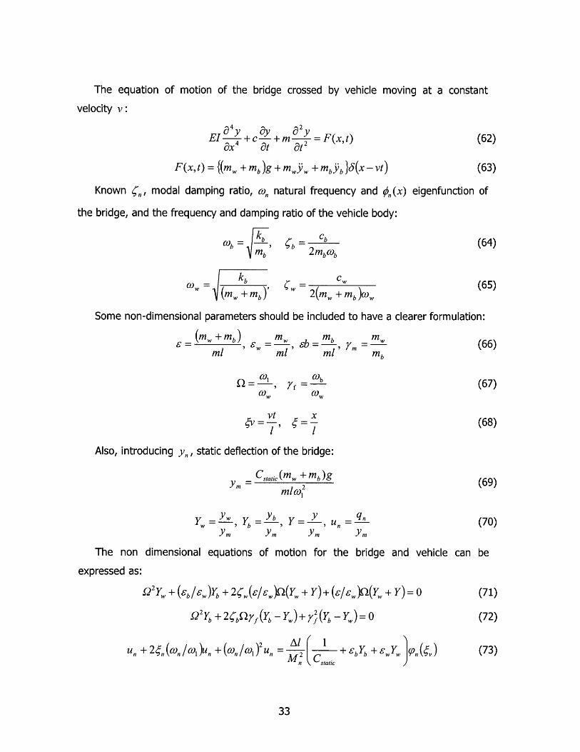
The equation of motion of the bridge crossed by vehicle moving at a constant
velocity v:
EI +c-+m =F(x,t) (62)8x4 Ot 0t2
F(x, t) = {(mv + mb)9 + mJy + mbYb }8(x - vt) (63)
Known 4,, modal damping ratio, co, natural frequency and $(x) eigenfunction of
the bridge, and the frequency and damping ratio of the vehicle body:
jkbmb
(O kb(MW +Mb)'
b Cb2mbwb
C+w2(MW +mb )w
(64)
(65)
Some non-dimensional parameters should be included to have a clearer formulation:
= +mb) 6ml
m m~bMW b ml'Ml i
VtS = ,
72f =
(w
CO=
1
Also, introducing y,, static deflection of the bridge:
= Cs,ic,(mw + mb)g
M mlco
yw y , y-, YM YM YM YM
non dimensional equations of motion for the bridge and vehicle can be
expressed as:
Q2 Yw + (g /,)Y+ 2(e/c))Q(Yw+Y)+(e/ew) (Y,+Y )=0
2 + 2b,7 yf(Y -Y) ,)+f(Y -Y)= 0
u, + 2n(COw/c)u +( n /cI) 2un = (C + 6bYb + C Ywn (4)M,2 C,,aic
33
mb(66)
(67)
(68)
The
(69)
(70)
(71)
(72)
(73)

With A =1.0 for forced vibration and A =0.0 for free vibration.
The nondimensional vertical displacement of the bridge Y is:
Y({,t)=Iu,,(r)(O,() T=Ot (74)n=1
The response of the bridge with a TMD in its midpoint of the span:
m. EIL
x kz cz y
TMDz
Figure 13 Bridge with Tuned Mass Damper.
The equation of motion of the TMD is given in [5] as:
m Y+c (i -j)+k,(z - y) =0 (75)
While the force applied on the bridge by the vehicle acts at the contact point
between vehicle and bridge, the TMD inertia force acts at the center of the bridge [5]:
F(x, t)= {m, + mb)g + m~Y + mbyb - V) + (mg - mA)9X - (76)
Defining some parameters as:
z = , = m, 7z = (77)y,, ml co~
The equation of motion for the TMD is:
f2 Z + 24-zQ2(Z -Y)+ (Z-Y) )= 0 (78)
The equations of motion for the system in matrix form results is:
M+CP+ Kp =Q (79)
Where:
34

(6b leEw)o 2
00
- Acwly 1 (Mv)/M 2
- Ae ly 2 ( v)/M2
0
-Aeho 2 ( v )/ M 1
0
0
6)l9p, ( L/ 2)/M 1CZ,0?2 ( L12)I M2
0 2{,(E/-.)Q ,( ,)- 2 bQ 7f 2 gbQvf
0 00
0
0
0
z
0
0 - 0
0- 24,z2y0 (L/2)
0
2{w(c/ew)efiPJv)0
- 2, f22(L/2)
0
2(,n(o2 / col
0 (e/.)e(0,)0
- yz j(L/ 2)
(0, /w)20
0
00
A9 o,(,
A9 2 (v
Y,
z
U'
U2
(6/6w) 02(0v
0- y7 gy2 (L/2)
0
(CO2 / o 3
35
0 0 ...
0 0 ...0 0 ...
0
1
0
(80)0
1
02
7f0
0
0
(e/c.)-7f2
0
0
0
(81)
02
0
0
Cstatm12
CstatM2
(82)
(83)
(84)
)+ CZf p L/2)
+EZ 2JL12)

11.1. Tuning condition of the TMD:
There are many tuning conditions proposed, however, the most commonly used [7]is Den Hartog's optimum tuning condition [8]:
= , = C" (85)ml (+85)
- = )2 36 = 2mz co (86)(2
cc 8(1+6zY cc w(
TMD damping affects the dynamic response of the structures more extensively thanthe damping values of the structures [5]. The critical damping proposed by Tsai [9]keep away from response increase due to inadequate damper tuning and beatingphenomenon:
z = n + F (87)
The mass ratios ez E (0.01-0.04) are generally recommended [5].
36

11.2. Case study:
The formulation here shown, was presented by [5] in the same article we can find a
example of the effectiveness of the TMD:
L=50m
E = 3.303*1010 [N/M2]
m = 3852 [kg/m3]Damping ratio (%1) = 0.3
Vvezicie =90[m / sg]I =18.638 [M 4 ]
A = 11.332 [M 4 ]
Wheel TGV:
Locomotive
M = 2382 kg
k =1.0 e7
c=4e7
Body TGV:
Locomotive
M = 13,760 kg
k =5.0 e7
c=8e4
Semi-passenger
M =2382
k =2.35e6
c =4e4
Semi-passenger
M =17,000
k =2.86e6
c=8e4
Passenger car
M =2383
k =1.0e7
c=8e4
Passenger car
M =17,000
k =5.0e7
c=8e4
3.5 m
14 m
40 m 40 m
Figure 14. Bridge and vehicle's parameters [5]
37
40 m
U* 4

Comparisc
velocities:
1.10
+1 1.00
0.800.IU.u
50
in the response of the bridge under a TGV traveling with different
150 250 350Velocity, km/h
Figure 15. Maximum response at point x=L/2 at different velocities. Capture [5]
It is important to notice that the response with a smaller velocity can be higher. That
is because the loading space has its own speed which makes the bridge response
maximum. Therefore it is difficult to know a priori which velocity would produce the
maximum response, and it is necessary to try with different velocities to find the worst
case scenario.
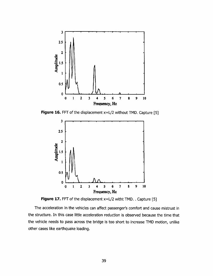
Comparison between the fast Fourier transform (FFT) for the bridge with and
without a TMD of mass ratio Ez = 0.01
38
450 550
n
3
2.5
2
1.5
I
0.5
A0 1 2 3 4 5 6
Frequency, Hz
Figure 16. FFT of the displacement x=L/2 without TMD. Capture [5]
3
2.5
2
~1.5
41
0.5
00 1 2 3 4 5 6 7
Frequency, Hz
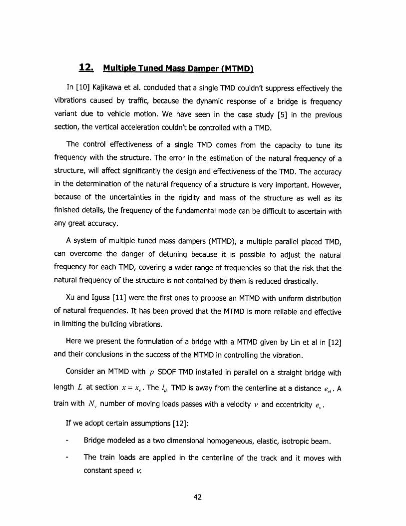
Figure 17. FFT of the displacement x=L/2 witht
8 9 10
TMD. . Capture [5]
The acceleration in the vehicles can affect passenger's comfort and cause mistrust in
the structure. In this case little acceleration reduction is observed because the time that
the vehicle needs to pass across the bridge is too short to increase TMD motion, unlike
other cases like earthquake loading.
39
I. .I % ? A
7 8 9 100

0.10
I.I
0.05
0.000.
-0.05
-0.10
Time, sec
Figure 18. Acceleration of the vehicle body. Capture [5]
0.10
0.05-
0.00
<-0.05
---- w/o TMD
--- w/ TMD-010
Time, semFigure 19. Acceleration of the wheel. Capture [5]
40
1 51
w/o TMD
w/ TMD

11.3. Conclusions:
We can draw from [5] important conclusions:
- There can be sub-critical speeds within the bridge design speed.
- The bridge impact factors must be changed to adequate levels considering the
response of the bridge under a train traveling at sub-critical speeds.
- TMD reduces in a 21% the vertical displacement and free vibration dies out
fast when a TGV passes.
41
12. Multiple Tuned Mass DamDer (MTMD)
In [10] Kajikawa et al. concluded that a single TMD couldn't suppress effectively thevibrations caused by traffic, because the dynamic response of a bridge is frequency
variant due to vehicle motion. We have seen in the case study [5] in the previous
section, the vertical acceleration couldn't be controlled with a TMD.
The control effectiveness of a single TMD comes from the capacity to tune itsfrequency with the structure. The error in the estimation of the natural frequency of a
structure, will affect significantly the design and effectiveness of the TMD. The accuracyin the determination of the natural frequency of a structure is very important. However,
because of the uncertainties in the rigidity and mass of the structure as well as itsfinished details, the frequency of the fundamental mode can be difficult to ascertain with
any great accuracy.
A system of multiple tuned mass dampers (MTMD), a multiple parallel placed TMD,
can overcome the danger of detuning because it is possible to adjust the naturalfrequency for each TMD, covering a wider range of frequencies so that the risk that thenatural frequency of the structure is not contained by them is reduced drastically.
Xu and Igusa [11] were the first ones to propose an MTMD with uniform distribution
of natural frequencies. It has been proved that the MTMD is more reliable and effective
in limiting the building vibrations.
Here we present the formulation of a bridge with a MTMD given by Lin et al in [12]
and their conclusions in the success of the MTMD in controlling the vibration.
Consider an MTMD with p SDOF TMD installed in parallel on a straight bridge with
length L at section x = x,. The It, TMD is away from the centerline at a distance esi. A
train with N, number of moving loads passes with a velocity v and eccentricity ev.
If we adopt certain assumptions [12]:
- Bridge modeled as a two dimensional homogeneous, elastic, isotropic beam.
- The train loads are applied in the centerline of the track and it moves with
constant speed v.
42
yL
-+ x
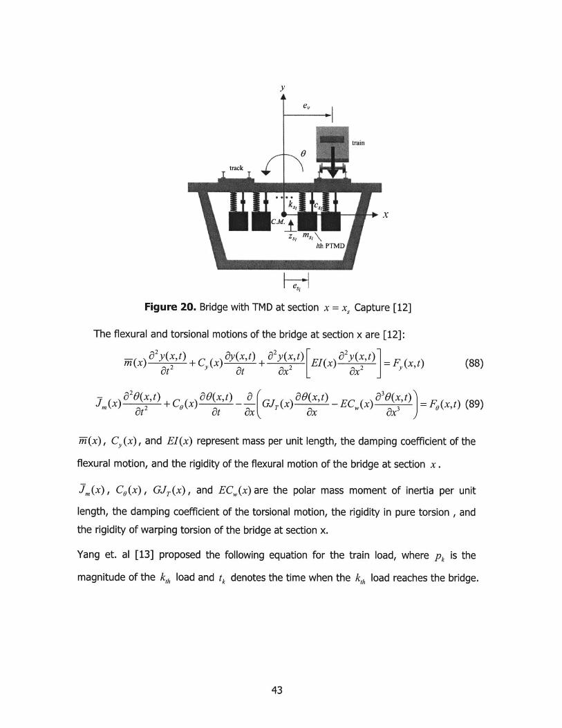
HHFigure 20. Bridge with TMD at section x = x, Capture [12]
The flexural and torsional motions of the bridge at section x are [12]:
a2 y(x, t) x y(xt) + 2 y(x,t)
at2 +C () at + x2 EI(x) a 2y(X, 0 = F (x, t)
,(x) a2 (xt) +J()at
2 + CO(x) aO(x,t) - GJr (x) xt) - ECa(x) a3 (xt) =ax ( a C(x ax3 ) F(x,t) (89)
ii(x), C,(x), and EI(x) represent mass per unit length, the damping coefficient of the
flexural motion, and the rigidity of the flexural motion of the bridge at section x.
J,(x), C9(x), GJT(x), and EC,(x) are the polar mass moment of inertia per unit
length, the damping coefficient of the torsional motion, the rigidity in pure torsion , and
the rigidity of warping torsion of the bridge at section x.
Yang et. al [13] proposed the following equation for the train load, where Pk is the
magnitude of the kh load and tk denotes the time when the kh load reaches the bridge.
43
(88)
A
F,(x,t) = -1 p9X - v(t - tk )]u( - t)k=1
(90)- y(x,, t) - es(x,, t)] + c,/ i - f(xS, t) - e,1d(x,, t)](x - x,)+ {kS, [z,1
i=I
The second term on the right hand side determines the location of the kh load on the
bridge, the third term determines whether the kh load is on the bridge or not
The FO proposed in [12]:
Nv
F(x,t) = -I evpk8[x -v(t -tk )i' -tk)k=1
+ ei=1
(91){ks, [z - y(x,,t) - e,,(xs,t)] +cs, [Zs - P(x,,t) -eld(x,,t)p(x - x,)
H(t,tk) = U(t-tk)-Ut-(tk + v/L)] , U(t) and 8(t) are the step function and the Dirac
delta function:
f18(x)dx= 1 :, X =0
10, Xw 0
U(t) = 130, t <O
(92)
(93)
The vertical motion of the ih TMD is:
m5,25,(t)+ c,1j*, -.j(x,,t) -es, 1 (x,,t)]+kl[z,, -y(x,,t) -es,0(x,,t)]= 0
Ms, cs,, and k, I are the mass, damping coefficient, and stiffness coefficient of the it
TMD, y(x,t) , O(x,t) and zI(t) indicate the vertical displacement of the bridge, the
torsional angle of the bridge, and the vertical displacement of the i,, TMD, respectively.
The pk depend on the train model. Depending on the level of complexity we want the
problem to have, the train can be considered as:
- Force model:
44
(94)

Pk =mMg (95)
- Mass model:
Pk = mk{g+ ,(t)} (96)
- Moving suspension mass model where the wheel masses are neglected:
Ak Mvk [g + zt) (97)
kxh load
Figure 21. Bridge with the three models of loads: force, moving mass andsprung moving mass. Capture [12]
mk ad z,(t) are the mass and the vertical displacement of the k,, train.
Modal analysis is employed to separate the governing parameters [12]:
N
y(x,t) = L #j(x)q1 (t) = I'(x)7(t) (98)]=1
N
9(x,t) = XL' 1 (x)7 1 (t) =yT(x)y(t) (99)j=1
N = number of nodes to be considered
0'(x)={#A(x), (x)...N(x)}, and T (x)={yI(X), 2(x)...N(X)} mode shape vectors.
45

/(t) and 1(t) are the modal-response vectors.
ve,(t) = zl(t)-y(x,, t)-eO(x,, t) is the stroke, the displacement of the Ith TMD relative to
the bridge where the 1,h TMD is located.
If we plug equations (90), (91), (98) and (99) in equations (88) and (89) and we
premultiplying 1(x), I(x), we get in matrix form:
My7j(t) + C,6(t + KYq(t) = Fv(t) + FMTMD(t)
Moij(t) + Coi(t) + K07r(t) = F6 (t) + FMTMD(t)
Where My, MO , C, , C0 and K, , K0 are N * N matrices, representing modal
mass, damping and stiffness of the bridge flexural motion and of the bridge torsional
motion respectively. After the application of ID(x) , P(x) , we get N uncoupled
equations:
qj (t)+2g .co Q(t) + cor(t) = F (t) + FTMD(t)
y1 (t) + 2 f,(t) + oyj (t) = F; (t) + FM TM D (t)
(102)
(103)
cow= kg1/my 3 and gj=c,/2mYcoj are the Jih flexural modal frequency and
damping ratio of the bridge
OO = k /m. and O = c./2mwc, are the j,, torsional modal frequency and
damping ratio of the bridge and:
m1 = f -(x)# (x)dx, , = .. .J(X)Y (x)dx,
c = f CY(x) (x)dx,
ky1 = f EI(x)#(x),
C= rC(x)V2(x)dx,
k,= JT(x) , (x)I +EC,(x)y4(x) I x,
The j, flexural modal force F , and torsional modal force F;:
F. 1 E=1 (vt -vtk)H(t,k=1 Myj it
46
(100)
(101)
(104)
(105)
(106)
(107)

(108)Fv--vNv P
FMTDE = -eW (Vt -v t)Hy(t,tk=1 MO
FI'I" = P p,, +<n, O)2V/
FJAITM = 2{p,9,P=
(109)
(110)
and p = #jx,)m,,/mO are ratios of the 1 TMD mass
to the j,,, flexural and torsional modal mass of the bridge
The equation (94) can be rearranged into the displacement of the Ith TMD:
[p,(t) + (DT(xs)i (t) + esYT (x)(t) + 24,pwj's,5(t) + co2 vS, (t) = 0
If we express the equations of motion in matrix form:
M, y0
-M, S
K,,+ 0
-0
0 0 ij(t) ~C[,Moo 0 +(t) + 0
M,0 M, j, (t) [ 0
0 K,
K KI 21(t)0 K,_ vs()
0
COO0
C iCO
CS
F,,(t)
=F(t)-l0J
I(111)
(112)
where 0 is the null matrix and :
[, (x,)
# 2 (X, )
0N,
(xs)e
[ V2 (X, )es
YN (x, )e,
$A (x,)
S(x, )e 2K' (Xs )e, 2V/2 (X, )e 2
.(s~s
- -- 1(x,)1'.. 02 (Xs )
.. N (,
''' (x)e
''' V2(X,)esp
V' N,(x )eSP
47
Also:
Where psly = $/x,)m,,/m,,
+ CWlIVI S
(113)
(114)

- 2 ,,cos psly,
C - 2 s,,AP Ay2C,, = :
2 2,10 ps /SyN
- 2 so2s2s2
- 2 s2)s2JPs2YN
--- 25,,co,,py 1
2SPWSPuSPYIN
- 2 so~sjsj~j -2
s2LWs2Is2o]
-2 p 02 - 2 s2ps2s0 2
K- 2 so slpION - 2 s2WsA2SN
2 2-- ]Ps171 - Os2 Ps2Y
2 2[OPY - Ws2/is2Y2
2 2- 1sIYN - Ws2/s2YN
-JS2, /Is10,.
- w21Ps102
-w51psO
- c2Ps01
- C022Ps02
2s2Ps20N
-- 2 Sp,, PP01-- 2 sp,, sp02
2 sp sp Psp ON
sp spY 2
(0S2 /I
sp' sp N
(tw2~~
P s NJ
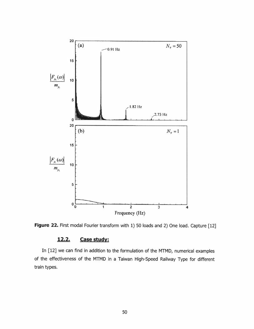
12.1. Dynamic of the load
A train acts on a bridge like a series of similar repetitive loads. This loading is like a
steady impact on the bridge if the train is moving with constant velocity [12], this will
have a different response that a bridge under a single vehicle load that only acts a short
time.
If the bridge is simply supported, the vertical vibration (D(x) is like we stated in
previous sections:
48
(115)
(116)
(117)
(118)

fD(x) sin , sin , ...sin l
If we do the Fourier transform of F v(co)the jth flexural modal train load [12]:
F (o) =
= f "' _ N Pk j v -vt)H (t, ts tk=1 MyL
If e sin an (t, t )dt2;rk m, _ L _
If each moving load Pk has the same magnitude and the same spacing d :
m CO2Lj () 2
1 -L
F (co) would be large as:
- sin(cod/2v) ~ 0
- or co = 2rnv / d (n = 1,2,...) where v /d is the impact frequency of the wheels
The bridge will have resonant speeds at:
V - 2(122)2nrc
The resonance does not only occur when the train travels at high speeds, also:
V = wL (123)nr '- -- I
The major critical condition (n = 1) only occur when the train speed is several times
the first resonant speeds; this is almost impossible for general high-speed railway
bridges [12], [13]. A single car passing through a bridge will not produce any resonant
response.
49
(119)
(120)
(121)
LFv (t)e- dt
sin WNv 2vW2v 2v ) (-1Ye-''"L/v 1
sin - -2v_
20(a) -0.91 Hz N, =50
16
6
1.82 Hz
.2,73 IIz
20
(b) NV,
16
10
00 1 2 3 4
Frequency (Hz)
Figure 22. First modal Fourier transform with 1) 50 loads and 2) One load. Capture [12]
12.2. Case study:
In [12] we can find in addition to the formulation of the MTMD, numerical examplesof the effectiveness of the MTMD in a Taiwan High-Speed Railway Type for differenttrain types.
50

0.23 wihmt ~4ThIf)
wtbmkt WTMI
Gem" .CE I26
0,24
0 20
0 14
Dr 12
Od ,
032 IF
Prench T.G.V
0)4
O Iiatso 100 ISO 200 260 300 3M
Train speed (kmh)50 100 15 200 20
Train speed (knh)
Figure 23. Maximal displacement and accelerations for a Taiwan High-Speed Train withand without MTMD. Capture [12]
51
0 6
0. 4
04ci
D. 00
wdh MTMD pr?
E-1 %M
01%
E
E
Jupaneg S.KS,
0C0
004
002
JraIKae S .K21
Prenda TV.
300tj UU
D, 06

12.3. Conclusions:
Important conclusions for the design of bridges can be derived from [12]:
- If the natural frequencies of the bridge are multiples of the impact frequency of the
of the train, the resonant effect will take place, although the train doesn't travel at high
speeds.
- The MTMD can control effectively the dynamic response of the bridge and train
only if are dominated by the resonant response within the design train speed.
- The error in the estimation of the bridge frequencies and the bridge-train
interaction will affect the control effectiveness of a single TMD. However a MTMD
system with the same mass but a wider range of frequencies, is less affected by the
detuning effect, being more reliable and robust than a single TMD.
52

13. References
[1] F T K Au, Y S Cheng and Y K Cheung. Vibration analysis of bridges undermoving vehicles and trains: an overview. Progress in Structural Engineering andMaterials Volume 3, Issue 3 , Pages 299 - 304
[2] Yeong-bin Yang, Chia-Hung Chang and Jong-Dar Yau. An element foranalyzing vehicle-bridge systems considering vehicle's pitching effect. InternationalJournal for Numerical Methods in Engineering 1999: 46: 1031-1047
[3] H-T Lin and S-H Ju Three-dimensional analyses of two high-speed trainscrossing on a bridge. Proceedings of the Institution of Mechanical Engineers .2003Volume 217 Part F
[4] J. H. Biggs Introduction to Structural Dynamic. Mc Graw Hill, 1964.Page315-318
[5] Ho-Chui Kwon, Man-Cheoil Kim, In-Won Lee Vibration control of bridgesunder moving loads. Computer & Structures, 1998.Vol. 66, No 4, pp 473-480
[6] Y. K. Cheung, F. T. K. Au, D. Y. Zheng and Y. S. Cheng Vibration of multi-span non-uniform bridges under moving vehicles and trains by using modified beamvibration functions. Journal of Sound and Vibration, 1999.228(3), pp 611-628
[7] Bachmann, H. and Weber, B. Tuned vibration absorbers for lively structures.Journal of the International Association for Bridge and Structural Engineering (IABSE),1995.
[8] Hartog D. Mechanical vibrations. Dover Pub/ications, New York, 1985
[9] Fryba L., Vibration of Solids and Structures under Moving Loads. DNoordhoffInternational, Groningen, The Netherlands, 1972
[10] Kajikawa, Y., Okino,M., Uto, S., Matsuura, Y., and Iseki, J. Control oftraffic vibration on urban viaduct with tuned mass dampers. Journal of StructuralEngineering, 35(A), 585-595, 1989.
[11] Xu, K., and Igusa, T. Dynamic characteristics of multiple substructures withclosely spaced frequencies. Earthquake Eng Structural Dynamics, 21, 1059-1070, 1992.
[12] C. C.Lin, M.ASCE, J.F. Wang, and B.L. Chen. Train-Induced VibrationControl of High-Speed Railway Bridges Equipped with Multiple Tuned Mass Dampers.Journal of Bridge Engineering, ASCE, July-August, 398-414, 2005.
[13] Yang, Y.B., Yau, J. D., and Hsu, L. C. Vibration of simple beams due totrain movement at high speeds. Engineering Structural, 19 (11), 936-944, 1997.
53

APPENDIX A:
MATLAB CODE TO GET THE ANALYTICAL DEFORMATION AT ANY GIVENPOINT UNDER A MOVING LOAD
L=5 0
n=1000 %number of nodes
xcontrol =5*L/10 ; %Point of beam where deflection is analysed
v= 90 %velocity of the train in m/sg
F= -1 %Weight of the force
m=43651.935 %[kg/m] Linear density
E=3.303e10 %Young Modulus [N/m2]
I=18.638 %Moment of inertia [m4]
timestep = 0.001
T=[0:timestep:L/v] %Range of t in which I see the response
y=zeros(size(T)) '; %Column vector
for i=1:n ;
Wn=i*pi*v/L;
wn=i^2*pi^2/L^2* (E*I/m)A0 .5;
deltay=2*F/ (m*L) / (wn^2-WnA2) * (sin (Wn*T)
-Wn/wn*sin(wn*T'))*sin(i*pi*xcontrol/L);
y=y+deltay;
end
plot (T,y, 'r-')
hold on
end
54

APPENDIX B:
MATLAB CODE TO GENERATE A DYNAMIC AMPLIFICATION FACTOR
%%% Generation of dynamic amplification factor curve %%%%%
hold off
n=1 % Mode in which I am looking the dynamic amplification factor
% Number of curves that I get with the parameter v/L
curve0 = 0.2 % Initial curve
curvefin = 1 % Final curve
curvestep = 0.01 % Interval of the curves
curves= [curveO:curvestep:curvefin] % Vector that stores the vL parameters
% The x axis:
xO= 0.02 % Where x starts
minunitaxis = 0.01 ; % Minimum unit of x
xfin = 0.4 % Where x finishes
% IMPORTANT!! xfin = x0 + q* minutaxis with q integer
x-axis = [xO:minunitaxis:xf in] ; % Axis vector adimensional (E*I/m)^0.5/L^2
% The y axis stored for each x
DLF = zeros(size(curves),size(xaxis)); % Matrix in which
% amplification factors will be stored
% Each row is the DLF for a given relation
timestep= 0.001
for p = 1:(curvefin-curve0)/curvester-
v_L = curves(p)
for j=1:(xfin-xO)/minunitaxis+l
timestep = 1/(100*vL);
T=[0:timestep:1/vL];
ck = x_axis(j)
Wn=n*pi*vL;
wn=n^2*pi^2*ck;
the dynamic
of v/L relation
% We do a cycle for each curve
%Range of t in which I see the response
DLFT=1/(wn^2-Wn^2)*(sin(Wn*T)-Wn/wn*sin(wn*T));
DLF (p,j)= max(abs(DLFT));
55

end
end
for q=l:(curvefin-curveO)/curvestep +1
cur = DLF(q,:)
figure(8);
plot(xaxis,cur,'k-')
hold on
end
end
56