MPRAMunich Personal RePEc Archive

Concave consumption function andprecautionary wealth accumulation

Suen, Richard M. H.

University of Connecticut

November 2011

Online at http://mpra.ub.uni-muenchen.de/34774/

MPRA Paper No. 34774, posted 16. November 2011 / 16:53

Concave Consumption Function and Precautionary

Wealth Accumulation�

Richard M. H. Sueny

First Version: August 2010

This Version: November 2011

Abstract

This paper examines the theoretical foundations of precautionary wealth accumulation in a multi-

period model where consumers face uninsurable earnings risk and borrowing constraints. We begin

by characterizing the consumption function of individual consumers. We show that consumption

function is concave when the utility function has strictly positive third derivative and the inverse

of absolute prudence is a concave function. These conditions encompass all HARA utility functions

with strictly positive third derivative as special cases. We then show that when consumption function

is concave, a mean-preserving spread in earnings risk would encourage wealth accumulation at both

the individual and aggregate levels.

Keywords: Consumption function, borrowing constraints, precautionary saving

JEL classi�cation: D81, D91, E21.

�An earlier version of this paper is circulated under the title �Concave Consumption Function under Borrowing Con-straints.�I would like to thank Alan Binder, Christopher Carroll, Jang-Ting Guo, Miles Kimball, Carine Nourry, seminarparticipants at the University of Connecticut and UC Riverside, conference participants at the 2011 Symposium of SNDE,the 2011 T2M Conference and the 2011 North American Summer Meetings of the Econometric Society for helpful com-ments and suggestions.

yDepartment of Economics, 341 Mans�eld Road, Unit 1063, University of Connecticut, Storrs CT 06269-1063, UnitedStates. Email: richard.suen@uconn.edu. Phone: 1 860 486 4368. Fax: 1 860 486 4463.

1

1 Introduction

This paper analyzes the optimal life-cycle saving behavior of risk-averse consumers who face uninsurable

idiosyncratic earnings risk and borrowing constraints. The purpose of this study is to better understand

the theoretical foundations of precautionary wealth accumulation. In particular, this study seeks to

provide conditions under which an increase in the riskiness of earnings would lead to an increase in

both individual and aggregate savings. Unlike most of the existing studies, we do not restrict our

attention to HARA utility functions.1 Instead, we explore general conditions on preferences under

which precautionary saving would emerge.

Precautionary saving behavior has long been the subject of both empirical and theoretical studies.

Recent empirical work show that precautionary saving plays a crucial role in explaining wealth accu-

mulation over the life cycle.2 In the theoretical literature, a large number of studies have analyzed

the optimal response of saving to uninsurable income risk.3 One intriguing �nding from these studies

is that precautionary saving behavior is closely related to the concavity of the consumption function.

Intuitively, concavity means that there is an inverse relationship between the marginal propensity to

consume and the total resources available for consumption. Thus, when facing the same �uctuation in

earnings, poor consumers would have a larger response in consumption than rich consumers. This in

turn implies a higher consumption volatility for the poor than the rich. Since risk-averse consumers dis-

like volatility in consumption, this creates an incentive for them to accumulate more wealth.4 Huggett

(2004) provides the �rst formal proof on the connection between concave consumption function and

precautionary wealth accumulation. Using a canonical life-cycle model with purely transitory earnings

risk, Huggett shows that when the consumption function is concave, an increase in earnings risk would

induce each consumer to accumulate more assets. This in turn raises the average level of wealth at

each stage of the life cycle.

Huggett�s result suggests that one way to improve our understanding of precautionary saving be-

havior is to identify the conditions under which consumption function is concave.5 Due to a lack of

1HARA is the acronym for hyperbolic absolute risk aversion. The HARA class of utility functions include some ofthe most commonly used utility functions in the existing studies, such as the constant-absolute-risk-aversion (CARA)utility function, the constant-relative-risk-aversion (CRRA) utility function, and the quadratic utility function. A formalde�nition of HARA utility function is stated in Section 3.3.

2See, for instance, Carroll and Samwick (1997, 1998), Gourinchas and Parker (2002), and Parker and Preston (2005).For a comprehensive survey of some earlier studies, see Browning and Lusardi (1996).

3Huggett (2004) provides an excellent review on some of the early studies. Heathcote et al. (2009) provide an extensivesurvey of the models with idiosyncratic risks and incomplete markets.

4See Carroll (1997) for more discussion on the implications of concave consumption function.5This also raises the natural question of whether concave consumption function is consistent with empirical evidence.

2

closed-form solutions, existing studies typically rely on computational methods to derive the consump-

tion function. Zeldes (1989), Deaton (1991) and Carroll (1992, 1997) are among the �rst studies that

use these methods to show that consumption function is concave under constant-relative-risk-aversion

utility. Carroll and Kimball (1996) is the �rst study that provides a rigorous analysis on this subject.

These authors show that, in the absence of borrowing constraints, consumption function exhibits con-

cavity when the utility function is drawn from the HARA class and has strictly positive third derivative.

Huggett (2004) and Carroll and Kimball (2005) extend this result to an environment with borrowing

constraints, while maintaining the HARA assumption.

Although existing studies focus exclusively on HARA utility functions, there is no compelling the-

oretical or empirical reason to con�ne ourselves to this class of utility functions. Adopting the HARA

assumption is equivalent to assuming that consumers have linear absolute risk tolerance. There is no

empirical evidence concerning the linearity or the curvature of absolute risk tolerance. In the theory

of consumer preferences, the usual axioms do not imply a linear absolute risk tolerance. On the con-

trary, a growing number of studies show that the nonlinearity of absolute risk tolerance has important

implications in both deterministic and stochastic models.6 In the precautionary savings literature, it

remains an open question whether the existing results on concave consumption function are still valid

once we remove the HARA assumption. This paper provides the �rst general answer to this question.

In this paper, we consider a model economy in which a large number of ex ante identical consumers

face uninsurable idiosyncratic earnings risk and borrowing constraints over the life cycle. The exogenous

earnings process can be decomposed into a permanent component and a purely transitory component.

The consumers are identical before the earnings shocks are realized. In the �rst part of the analysis, we

provide a detailed characterization of the consumption function for individual consumers. The main

objective here is to derive a set of conditions on preferences such that the consumption function exhibits

concavity. In the second part of the analysis, we explore the connection between concave consumption

function and precautionary saving. In particular, we examine how changes in the riskiness of permanent

Using data from the Consumption Expenditure Survey, Gourinchas and Parker (2001) estimate the consumption functionfor U.S. households in various age groups and �nd that it is a concave function in liquid assets. Souleles (1999) andJohnson et al. (2006) examine the response of household consumption to income tax refunds and income tax rebates inthe United States. Both studies �nd that households with few liquid assets tend to have a larger propensity to consumethan those with more liquid assets, which is consistent with a concave consumption function.

6Gollier (2001) shows that the curvature of absolute risk tolerance is important in understanding the relationshipbetween wealth inequality and equity premium. Gollier and Zeckhauser (2002) show that this curvature is crucial inunderstanding how the length of investment horizon would a¤ect portfolio choice. Ghiglino and Venditti (2007) showthat, in a deterministic growth model, the curvature of absolute risk tolerance is a key factor in determining the e¤ect ofwealth inequality on macroeconomic volatility.

3

and transitory earnings shocks would a¤ect wealth accumulation at both the individual and aggregate

levels. Similar to Huggett (2004), we focus on the e¤ects of earnings risk on the average life-cycle pro�le

of wealth, which captures the cross-sectional average level of asset holdings at di¤erent stages of the

life cycle.

This paper presents two main �ndings. Our �rst major result states that, in the presence of

borrowing constraints, consumption function at every stage of the life cycle exhibits concavity if the

utility function has strictly positive third derivative and the inverse of absolute prudence is a concave

function.7 For any HARA utility function, the inverse of absolute prudence is a linear function. The

stated conditions thus include all HARA utility functions with strictly positive third derivative as

special cases. This makes clear that hyperbolic absolute risk aversion is not a necessary condition for

concave consumption function. When comparing to Huggett (2004) and Carroll and Kimball (2005),

our concavity result is applicable to a broader class of utility functions. For HARA utility functions,

we show that the consumption function is strictly concave in the permanent component of the earnings

shock when the borrowing constraint is not binding. This implies that the marginal propensity to

consume out of permanent shock is less than unity and is strictly decreasing in the level of the shock.

This provides a formal proof for the numerical �ndings in Carroll (2009).8 Our second major result

states that, when the consumption function at every stage of the life cycle is concave, a mean-preserving

spread in either the permanent or transitory earnings shock would induce each consumer to accumulate

more assets. This in turn raises the average level of wealth at di¤erent stages of the life cycle. Since

all other factors (including prices) are held constant in this analysis, the increase in asset holdings is

entirely driven by the precautionary motive.

To show that these results are tight, we provide a set of numerical examples in which the utility

function has strictly positive third derivative but the inverse of absolute prudence exhibits local con-

vexity. We show that under certain parameter values the consumption function in certain period is

not globally concave. Using this result, we are able to construct examples in which a mean-preserving

spread in the transitory earnings shock would lead to a reduction in aggregate savings. These examples

show that if the inverse of absolute prudence is not globally concave, then precautionary saving may

7Following Kimball (1990), the coe¢ cient of absolute prudence for a thrice di¤erentiable utility function u (�) is de�nedas �(c) � �u000 (c) =u00 (c) : The concavity of the inverse of �(�) remains an open empirical question.

8Carroll (2009) numerically solves and simulates the standard bu¤er-stock saving model with CRRA utility function.He �nds that the marginal propensity to consume out of permanent earnings shock is less than unity over a wide range ofparameter values.

4

not occur even when the utility function has strictly positive third derivative.9

The current study is close in spirit to Huggett (2004). There are, however, two important di¤erences

between the two work. First, Huggett only considers purely transitory risk, while the present study

makes a distinction between permanent and transitory risks. We show that this distinction is important

in deriving the concavity results. Second, Huggett only considers HARA utility functions and does not

explore the possibility of having concave consumption function under more general utility functions.

Our results show that concave consumption function can be obtained even if we move beyond the

HARA class of utility functions.

This rest of this paper is organized as follows. Section 2 presents the model environment and

establishes some intermediate results. Section 3 establishes the concavity of the consumption function

and contrasts our result to those in the existing studies. Section 4 examines how changes in the riskiness

of permanent and transitory earnings risks would a¤ect individual and aggregate savings. Section 5

presents a set of numerical examples to illustrate the theoretical results. Section 6 concludes.

2 The Model

Consider an economy inhabited by a continuum of ex ante identical consumers. The size of population

is constant and is normalized to one. Each consumer faces a (T + 1)-period planning horizon, where

T is �nite. The consumers have preferences over random consumption paths fctgTt=0 which can be

represented by

E0

"TXt=0

�tu (ct)

#; (1)

where � 2 (0; 1) is the subjective discount factor and u (�) is the (per-period) utility function. The

domain of the utility function is given by D = [c;1) ; where c � 0 is a minimum consumption re-

quirement.10 The function u : D ! [�1;1) is once continuously di¤erentiable, strictly increasing and

strictly concave.11 There is no restriction on the value of u (c) ; which means the utility function can

9These examples also highlight an important di¤erence between two-period models and general multi-period models.It is well-known that in two-period models, precautionary savings emerge if and only if the utility function has strictlypositive third derivative. This result, however, is not true in models with more than two periods. We will discuss thispoint in greater detail in Section 4.10This speci�cation encompasses those utility functions that are not de�ned at c = 0: One example is the Stone-Geary

utility function which belongs to the HARA class and features a minimum consumption requirement. All the results inthis paper remain valid if we set c = 0:11None of the results in this section require higher order di¤erentiability of the utility function. These properties are

required only in later sections.

5

be either bounded or unbounded below.

In each period t 2 f0; 1; :::; Tg ; each consumer receives a random amount of labor endowment

et; which they supply inelastically to work. Labor income at time t is then given by wet; where

w > 0 is a constant wage rate. The stochastic labor endowment is determined by et = eet"t; whereeet is a permanent component and "t is a purely transitory component.12 The initial value of the

permanent component ee0 > 0 is given and is identical across all consumers. This component then

evolves according to eet = eet�1�t; where �t is drawn from a compact interval � � [�; �] ; with � > � > 0;

according to the distribution Lt (�) : Similarly, the transitory shock "t is drawn from a compact interval

� � ["; "] ; with " > " > 0; according to the distribution Gt (�) :13 Both Lt (�) and Gt (�) are well-

de�ned distribution functions, which means they are both nondecreasing, right-continuous and satisfy

the following conditions:

lim�!�

Lt (�) = lim"!"

Gt (") = 0 and lim�!�

Lt (�) = lim"!"

Gt (") = 1:

The random variables "t and �t are independent of each other, across time and across agents.

Under this speci�cation, knowledge on both eet and "t is required to determine the distribution

of et+1: Thus, an individual�s state at time t includes zt � (eet; "t) : Under the stated assumptions,the stochastic event zt � (eet; "t) follows a Markov process with compact state space Zt � �t � �;

where �t �h�t; �t

icontains all possible realizations of eet:14 Let (Zt;Zt) be a measurable space and

Qt : (Zt;Zt)! [0; 1] be the transition function of the Markov process at time t: For any z = (ee; ") 2 Ztand for any B � Zt+1;

Qt (z;B) � Pr f(�t+1; "t+1) 2 �� � : (ee�t+1; "t+1) 2 Bg :It is straightforward to show that the transition function in each period satis�es the Feller property.

In light of the uncertainty in labor income, the consumers can only self-insure by borrowing or

lending a single risk-free asset. The gross return from the asset is (1 + r) > 0:15 Let at denote asset

12This dichotomy between permanent and transitory income shocks is commonly used in quantitative studies. Examplesinclude Zeldes (1989), Carroll (1992, 1997, 2011), Ludvigson (1999), Gourinchas and Parker (2002), Storesletten et al.(2004a), among many others. Empirical studies on household earnings dynamics show that this speci�cation �ts the datawell. See, for instance, Abowd and Card (1989), Storesletten et al. (2004b), and Mo¢ tt and Gottschalk (2011).13The age-dependent nature of Lt (�) and Gt (�) can be used to capture any age-speci�c di¤erences in earnings across

consumers. Hence, we do not include a separate life-cycle component in et:14For any t 2 f0; 1; :::; Tg ; the upper and lower bounds of �t are given by �t � ee0�t and �t � ee0�t; respectively.15 In the existing studies, it is typical to assume that w and r are deterministic and time-invariant. The time-invariant

6

holdings at time t: A consumer is said to be in debt if at is negative. In each period t, the consumers

are subject to the budget constraint

ct + at+1 = wet + (1 + r) at; (2)

and the borrowing constraint: at+1 � �at+1: The parameter at+1 � 0 represents the maximum amount

of debt that a consumer can owe at time t: The borrowing limits are period-speci�c (or, more precisely,

age-speci�c) for the following reason. In life-cycle models, consumers are typically forbidden to die in

debt. Thus, the borrowing limit in the terminal period must be aT+1 = 0: But the borrowing limit

in all other periods can be di¤erent from zero. Throughout this paper, we maintain the following

assumptions on the borrowing limits: at � 0; for all t; aT+1 = 0 and

wet � (1 + r) at + at+1 > c; for all t; (3)

where et � �t� " is the lowest possible value of et: The intuitions of (3) are as follows. Consider a

consumer who faces the worst possible state at time t; i.e., at = �at and et = et: The highest attainable

consumption in this particular state is ct = wet � (1 + r) at + at+1: Condition (3) then ensures that a

consumer can meet the minimum consumption requirement even in the worst possible state. The same

condition also ensures that any debt at time t can be repaid in the future even if a consumer receives

the lowest labor income in all future periods, i.e.,

T�tXj=0

wet+j � c(1 + r)j

� (1 + r) at > 0; for all t:

2.1 Consumers�Problem

Given the prices w and r, the consumers�problem is to choose sequences of consumption and asset

holdings, fct; at+1gTt=0 ; so as to maximize the expected lifetime utility in (1), subject to the budget

constraint in (2), the minimum consumption requirement ct � c; the borrowing constraint at+1 � �at+1for all t; and the initial conditions: a0 � �a0 and ee0 > 0:assumption is not essential for our results. Speci�cally, all of our proofs can be easily modi�ed to handle any pricesequences fwt; rtgTt=0 that are deterministic, bounded above and strictly positive.

7

De�ne a sequence of assets fatgTt=0 according to

at+1 = wet + (1 + r) at � c; for all t;

where et � �t � " is the highest possible value of et, and a0 = a0: This sequence speci�es the amount

of asset available in every period for a consumer who receives the highest possible labor income wet

and consumes only the minimum requirement c in every period. Since (1 + r) > 0; this sequence is

monotonically increasing and bounded above by

aT � (1 + r)T a0 +T�1Xj=0

(1 + r)T�1�j (wej � c) ;

which is �nite as T is �nite. It is straightforward to show that any feasible sequence of assets fatgTt=0must be bounded above by fatgTt=0 : Hence, the state space of asset in every period t can be restricted

to the compact interval At = [�at; at] :

In any given period, the state of a consumer is summarized by s = (a; z) ; where a denotes his

asset holdings at the beginning of the period, and z � (ee; ") is the current realization of the earningsshocks.16 The set of all possible states at time t is given by St = At � Zt:

De�ne a set of value functions fVtgTt=0 ; Vt : St ! [�1;1] for each t; recursively according to

Vt (a; z) = maxc2[c;x(a;z)+at+1]

(u (c) + �

ZZt+1

Vt+1�x (a; z)� c; z0

�Qt�z; dz0

�); (P1)

where x (a; z) � we (z) + (1 + r) a and e (z) is the level of labor endowment under z � (ee; ") : Thevariable x (a; z) is often referred to as cash-in-hand in the existing studies. In the terminal period, the

value function is given by

VT (a; z) = u [we (z) + (1 + r) a] ; for all (a; z) 2 ST :

De�ne a set of optimal policy correspondences for consumption fgtgTt=0 according to

gt (a; z) � argmaxc2[c;x(a;z)+at+1]

(u (c) + �

ZZt+1

Vt+1�x (a; z)� c; z0

�Qt�z; dz0

�); (4)

16For the results in this section, the distinction between ee and " is immaterial. Thus, we express individual state ass = (a; z) ; instead of s = (a; ee; ") ; throughout this section.

8

for all (a; z) 2 St and for all t: Given gt (a; z) ; the optimal choices of at+1 are given by

ht (a; z) ��a0 : a0 = x (a; z)� c; for some c 2 gt (a; z)

: (5)

Our �rst theorem summarizes the main properties of the value functions. The �rst part of the

theorem states that the value function in every period t is bounded and continuous on St. This is true

even when the utility function u (�) is unbounded below. Boundedness of the value functions ensures

that the conditional expectation in (P1) is well-de�ned. Continuity of the objective function in (P1)

ensures that the optimal policy correspondence gt (�) is non-empty and upper hemicontinuous. The

second part of the theorem establishes the strict monotonicity and strict concavity of Vt (�; z) : Strict

concavity of Vt (�; z) then implies that gt (�; z) and ht (�; z) are single-valued functions for all z 2 Zt:

The last part of the theorem establishes the di¤erentiability of Vt (�; z) : Speci�cally, this result states

that Vt (�; z) is not only di¤erentiable in the interior of At; but also (right-hand) di¤erentiable at the

endpoint �at: This property is important because, as is well-known in this literature, a consumer may

choose to exhaust the borrowing limit in certain states.17 In other words, the consumers�problem may

have corner solutions in which ht�1 (a; z) = �at for some (a; z) 2 St�1: Thus, the �rst-order condition

of (P1) has to be valid even when ht�1 (a; z) = �at. This requires the value function Vt (�; z) to be

right-hand di¤erentiable at a = �at: Note that the standard result in Stokey, Lucas and Prescott (1989)

Theorem 9.10 only establishes the di¤erentiability of the value function in the interior of the state space.

Thus, additional e¤ort is needed to establish this result.18

Additional conditions are imposed in part (iii) of Theorem 1 to ensure that gt (a; z) > c for all

(a; z) 2 St: Speci�cally, the proof of part (iii) uses an intermediate result which states that if the utility

function satis�es the Inada condition u0 (c+) � limc!c+

u0 (c) = +1; or the consumers are impatient so

that � (1 + r) � 1; then it is never optimal to consume only the minimum consumption requirement

c:19 The intuition of the Inada condition is well understood. When � (1 + r) � 1; the loss in utility

incurred by reducing current consumption to c is always greater than the gain from increased future

17This result is formally proved in a number of studies, including Mendelson and Amihud (1982), Aiyagari (1994),Huggett and Ospina (2001) and Rabault (2002).18Another related point is that Vt (�; z) is di¤erentiable on [�at; at) even if the policy function gt (�; z) is not di¤erentiable

at the point where the borrowing constraint becomes binding. For a more detailed discussion on this, see Schechtman(1976) p.221-222.19The same assumption is also used in Huggett (2004). In the bu¤er-stock savings model pioneered by Deaton (1991)

and Carroll (1992, 1997), it is typical to assume that consumers are impatient so that � (1 + r) � 1: It is also possible toavoid this type of corner solution by imposing u (c) = �1:

9

consumption. Hence, it is never optimal to choose c: It follows that ht (a; z) can never reach the upper

bound at+1 in any period t: Hence, there is no need to consider corner solutions in which ht�1 (a; z) = at;

and the (left-hand) di¤erentiability of Vt (�; z) at a = at: Unless otherwise stated, all proofs can be found

in Appendix A.

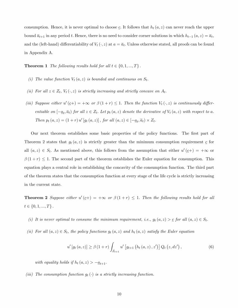
Theorem 1 The following results hold for all t 2 f0; 1; :::; Tg :

(i) The value function Vt (a; z) is bounded and continuous on St:

(ii) For all z 2 Zt; Vt (�; z) is strictly increasing and strictly concave on At:

(iii) Suppose either u0 (c+) = +1 or � (1 + r) � 1: Then the function Vt (�; z) is continuously di¤er-

entiable on [�at; at) for all z 2 Zt: Let pt (a; z) denote the derivative of Vt (a; z) with respect to a.

Then pt (a; z) = (1 + r)u0 [gt (a; z)] ; for all (a; z) 2 [�at; at)� Zt:

Our next theorem establishes some basic properties of the policy functions. The �rst part of

Theorem 2 states that gt (a; z) is strictly greater than the minimum consumption requirement c for

all (a; z) 2 St: As mentioned above, this follows from the assumption that either u0 (c+) = +1 or

� (1 + r) � 1: The second part of the theorem establishes the Euler equation for consumption. This

equation plays a central role in establishing the concavity of the consumption function. The third part

of the theorem states that the consumption function at every stage of the life cycle is strictly increasing

in the current state.

Theorem 2 Suppose either u0 (c+) = +1 or � (1 + r) � 1: Then the following results hold for all

t 2 f0; 1; :::; Tg :

(i) It is never optimal to consume the minimum requirement, i.e., gt (a; z) > c for all (a; z) 2 St:

(ii) For all (a; z) 2 St; the policy functions gt (a; z) and ht (a; z) satisfy the Euler equation

u0 [gt (a; z)] � � (1 + r)

ZZt+1

u0�gt+1

�ht (a; z) ; z

0��Qt �z; dz0� ; (6)

with equality holds if ht (a; z) > �at+1:

(iii) The consumption function gt (�) is a strictly increasing function.

10

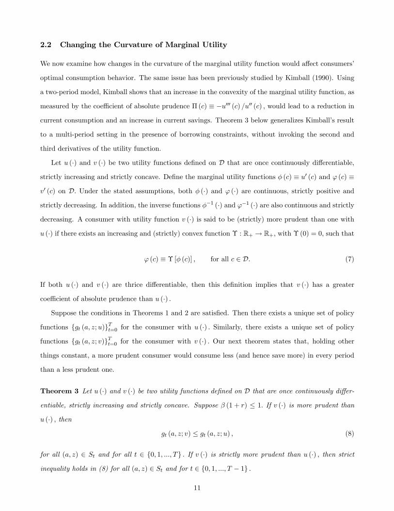
2.2 Changing the Curvature of Marginal Utility

We now examine how changes in the curvature of the marginal utility function would a¤ect consumers�

optimal consumption behavior. The same issue has been previously studied by Kimball (1990). Using

a two-period model, Kimball shows that an increase in the convexity of the marginal utility function, as

measured by the coe¢ cient of absolute prudence �(c) � �u000 (c) =u00 (c) ; would lead to a reduction in

current consumption and an increase in current savings. Theorem 3 below generalizes Kimball�s result

to a multi-period setting in the presence of borrowing constraints, without invoking the second and

third derivatives of the utility function.

Let u (�) and v (�) be two utility functions de�ned on D that are once continuously di¤erentiable,

strictly increasing and strictly concave. De�ne the marginal utility functions � (c) � u0 (c) and ' (c) �

v0 (c) on D: Under the stated assumptions, both � (�) and ' (�) are continuous, strictly positive and

strictly decreasing. In addition, the inverse functions ��1 (�) and '�1 (�) are also continuous and strictly

decreasing. A consumer with utility function v (�) is said to be (strictly) more prudent than one with

u (�) if there exists an increasing and (strictly) convex function � : R+ ! R+; with �(0) = 0; such that

' (c) � � [� (c)] ; for all c 2 D: (7)

If both u (�) and v (�) are thrice di¤erentiable, then this de�nition implies that v (�) has a greater

coe¢ cient of absolute prudence than u (�) :

Suppose the conditions in Theorems 1 and 2 are satis�ed. Then there exists a unique set of policy

functions fgt (a; z;u)gTt=0 for the consumer with u (�) : Similarly, there exists a unique set of policy

functions fgt (a; z; v)gTt=0 for the consumer with v (�) : Our next theorem states that, holding other

things constant, a more prudent consumer would consume less (and hence save more) in every period

than a less prudent one.

Theorem 3 Let u (�) and v (�) be two utility functions de�ned on D that are once continuously di¤er-

entiable, strictly increasing and strictly concave. Suppose � (1 + r) � 1: If v (�) is more prudent than

u (�) ; then

gt (a; z; v) � gt (a; z;u) ; (8)

for all (a; z) 2 St and for all t 2 f0; 1; :::; Tg : If v (�) is strictly more prudent than u (�) ; then strict

inequality holds in (8) for all (a; z) 2 St and for t 2 f0; 1; :::; T � 1g :

11

The interpretation of Theorem 3 depends crucially on the value of � (1 + r) : When � (1 + r) < 1;

an increase in the convexity of the marginal utility function has two e¤ects on consumption, namely

intertemporal substitution e¤ect and precautionary e¤ect. The former is evident from the fact that

Theorem 3 holds even in a deterministic environment.20 When � (1 + r) = 1; the curvature of the

marginal utility function has no e¤ect on consumption in a deterministic environment. In this case, the

result in Theorem 3 is purely driven by the precautionary e¤ect. The results in this section thus illustrate

a close relationship between the convexity of the marginal utility function and the precautionary motive

of saving. Speci�cally, a more convex marginal utility function implies a stronger precautionary motive.

3 Concavity of Consumption Function

3.1 Main Theorem

In this section, we provide a set of conditions on the utility function u (�) such that the consumption

function at every stage of the life cycle exhibits concavity. From this point onwards, we will focus on

utility functions that are thrice continuously di¤erentiable, strictly increasing and strictly concave. The

main results of this section are summarized in Theorem 5. These results cover two groups of utility

functions: (i) quadratic utility functions, or those with u000 (c) = 0 throughout the domain D; and (ii)

utility functions with strictly positive third derivative throughout its domain. For the latter class of

utility functions, an additional condition is needed in order to establish the desired result. It is shown

that this additional condition is satis�ed by a large class of utility functions, including (but is not

limited to) all HARA utility functions with strictly positive third derivative.

Recall that � (�) is the marginal utility function, i.e., � (c) � u0 (c) for c 2 D: If the utility function

is thrice di¤erentiable with nonzero third derivative, then we can de�ne � : D ! R according to

� (c) =

��0 (c)

�2�00 (c)

� [u00 (c)]2

u000 (c); (9)

and � : R+ ! R according to

� (m) � ����1 (m)

�: (10)

Both � (�) and � (�) are strictly positive if u000 (�) is strictly positive. Within this group of utility

functions, we con�ne our attention to those that satisfy the following assumption.

20See the proof of Theorem 3 for more discussion on this point.

12

Assumption A Let N > 1 be a positive integer. Let � be a discrete probability measure with

masses (�1; :::; �N ) on a set of points ( 1; :::; N ) 2 RN+ : Then the function � (�) de�ned by (9) and

(10) satis�es

�

"� (1 + r)

NXn=1

�n n

#� � (1 + r)

NXn=1

�n� ( n) : (11)

Before stating the main theorem, we �rst explain the implications of this assumption. We will

proceed in two steps. First, we identify a speci�c class of functions � (�) that are consistent with this

assumption. Next, we identify utility functions that can generate these � (�) :We begin with two special

cases. First, if � (m) � bm for some strictly positive real number b, then the condition in (11) holds

with equality for any � (1 + r) > 0: This seemingly trivial example turns out to have great importance.

In Section 3.3, it is shown that this simple form of � (�) encompasses all HARA utility functions with

strictly positive third derivative. Second, if � (1 + r) = 1; then the inequality in (11) becomes Jensen�s

inequality. Thus, any concave function � (�) is consistent with Assumption A. The following lemma

extends this result to the general case where � (1 + r) � 1; under the assumption that u000 (�) is strictly

positive.21 This result provides the basis for �nding a broader class of utility functions that satisfy

Assumption A. This will be explained more fully in Section 3.4.

Lemma 4 Suppose u000 (�) > 0 and � (1 + r) � 1: Let � : R+ ! R+ be the function de�ned by (9) and

(10). If � (�) is concave, then Assumption A is satis�ed.

We are now ready to state the main results of this section. Building on our earlier �ndings, Theorem

5 states that the consumption functions fgt (a; ee; ")gTt=0 are concave in (a; ee) and in (a; ") if the utilityfunction u (�) belongs to either one of the following categories: (i) quadratic utility functions, or (ii)

utility functions with strictly positive third derivative that satisfy Assumption A.

Theorem 5 Suppose the conditions in Theorem 2 are satis�ed. Suppose the utility function u (�) is

thrice continuously di¤erentiable, strictly increasing, strictly concave and satis�es one of the following

conditions: (i) u000 (�) = 0; or (ii) u000 (�) > 0 and Assumption A. Then the following results hold for all

t 2 f0; 1; :::; Tg :

(i) For any " 2 �; the consumption function gt (a; ee; ") is concave in (a; ee) :(ii) For any ee 2 �t; the consumption function gt (a; ee; ") is concave in (a; ") :21When � (1 + r) < 1; the inequality in (11) is not Jensen�s inequality. In particular, it is not satis�ed by all concave

functions � (�), but only by those with � (0) � 0: The additional requirement � (0) � 0 is ful�lled if u000 (�) > 0:

13

The proof of this theorem can be found in Section 3.2. Here we only provide a heuristic discussion on

the main ideas of the proof. As stated in Theorem 2, the set of consumption functions is characterized

by the Euler equation in (6). More speci�cally, using the consumption function in the terminal period

as the starting point, one can derive the consumption function in all preceding periods recursively using

the Euler equation. This essentially de�nes an operator which maps the consumption function at time

t+1 to that at time t:22 When the utility function is quadratic, the Euler equation is linear in both gt (�)

and gt+1 (�) : This, together with the fact that consumption function in the terminal period is linear in

(a; ee) and in (a; ") ; implies that the consumption function in all preceding periods are (piecewise) linearin (a; ee) and in (a; ") :23 For utility functions with strictly positive third derivative, Assumption A is

su¢ cient to ensure that the Euler operator preserves concavity. In other words, if gt+1 (�) is concave in

(a; ee) and in (a; "), then gt (�) is also concave in (a; ee) and in (a; ") :Three additional remarks are in order. First, Theorem 5 states that the consumption function

is jointly concave in current asset holdings and one of the income shocks, when the other is held

constant. In particular, gt (a; ee; ") is not jointly concave in (a; ee; ") : This happens because the stochasticlabor endowment e � ee" is not jointly concave in (ee; ") : Consequently, the consumption function inthe terminal period is not jointly concave in (a; ee; ") : It also means that the graph of the budgetcorrespondence Bt (a; ee; ") � �c : c � c � wee"+ (1 + r) a+ at+1 is not a convex set in any given period.Second, concavity in (a; ee) implies concavity in (a; ") ; but the converse is not true in general. Thispoint is explained more fully in Section 3.2. This result highlights the signi�cance of distinguishing

between permanent shock and purely transitory shock. Third, Theorem 5 only establishes the weak

concavity of the consumption functions. In Section 3.5, we present a set of su¢ cient conditions under

which the consumption functions are strictly concave in (a; ee) and in (a; ").3.2 Proof of Theorem 5

In this section, we focus on part (i) of the theorem. We will explain why this result implies the

result in part (ii) but not vice versa. The main ideas of the proof are as follows. For any " 2 � and22This is often referred to as the Euler operator. For a detailed characterization of this operator, see Deaton (1991) and

Rabault (2002).23 If the borrowing constraint is never binding, then the consumption function in any period t < T is linear in (a; ee) and

in (a; ") when the utility function is quadratic. If the borrowing constraint is binding in some states, then the consumptionfunction is kinked and piecewise linear in these arguments.

14

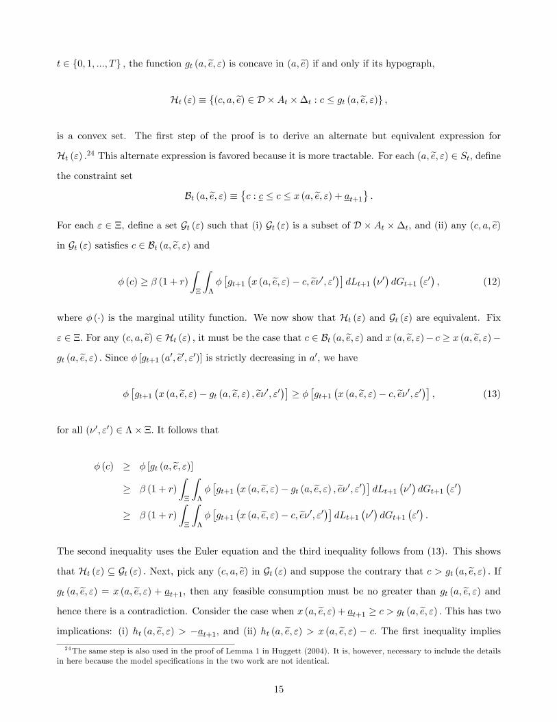
t 2 f0; 1; :::; Tg ; the function gt (a; ee; ") is concave in (a; ee) if and only if its hypograph,Ht (") � f(c; a; ee) 2 D �At ��t : c � gt (a; ee; ")g ;

is a convex set. The �rst step of the proof is to derive an alternate but equivalent expression for

Ht (") :24 This alternate expression is favored because it is more tractable. For each (a; ee; ") 2 St; de�nethe constraint set

Bt (a; ee; ") � �c : c � c � x (a; ee; ") + at+1 :For each " 2 �; de�ne a set Gt (") such that (i) Gt (") is a subset of D � At ��t; and (ii) any (c; a; ee)in Gt (") satis�es c 2 Bt (a; ee; ") and

� (c) � � (1 + r)

Z�

Z���gt+1

�x (a; ee; ")� c; ee� 0; "0�� dLt+1 �� 0� dGt+1 �"0� ; (12)

where � (�) is the marginal utility function. We now show that Ht (") and Gt (") are equivalent. Fix

" 2 �: For any (c; a; ee) 2 Ht (") ; it must be the case that c 2 Bt (a; ee; ") and x (a; ee; ")� c � x (a; ee; ")�gt (a; ee; ") : Since � [gt+1 (a0; ee0; "0)] is strictly decreasing in a0; we have

��gt+1

�x (a; ee; ")� gt (a; ee; ") ; ee� 0; "0�� � �

�gt+1

�x (a; ee; ")� c; ee� 0; "0�� ; (13)

for all (� 0; "0) 2 �� �: It follows that

� (c) � � [gt (a; ee; ")]� � (1 + r)

Z�

Z���gt+1

�x (a; ee; ")� gt (a; ee; ") ; ee� 0; "0�� dLt+1 �� 0� dGt+1 �"0�

� � (1 + r)

Z�

Z���gt+1

�x (a; ee; ")� c; ee� 0; "0�� dLt+1 �� 0� dGt+1 �"0� :

The second inequality uses the Euler equation and the third inequality follows from (13). This shows

that Ht (") � Gt (") : Next, pick any (c; a; ee) in Gt (") and suppose the contrary that c > gt (a; ee; ") : Ifgt (a; ee; ") = x (a; ee; ") + at+1, then any feasible consumption must be no greater than gt (a; ee; ") andhence there is a contradiction. Consider the case when x (a; ee; ") + at+1 � c > gt (a; ee; ") : This has twoimplications: (i) ht (a; ee; ") > �at+1; and (ii) ht (a; ee; ") > x (a; ee; ") � c: The �rst inequality implies

24The same step is also used in the proof of Lemma 1 in Huggett (2004). It is, however, necessary to include the detailsin here because the model speci�cations in the two work are not identical.

15

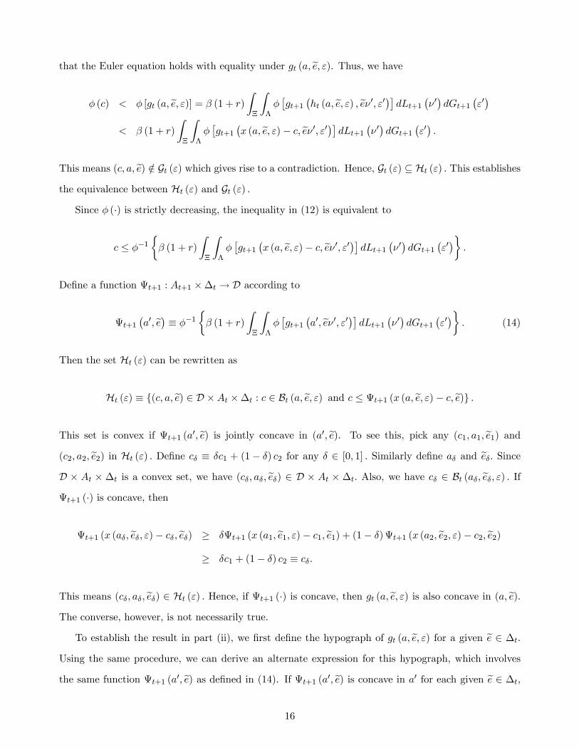
that the Euler equation holds with equality under gt (a; ee; "). Thus, we have� (c) < � [gt (a; ee; ")] = � (1 + r)

Z�

Z���gt+1

�ht (a; ee; ") ; ee� 0; "0�� dLt+1 �� 0� dGt+1 �"0�

< � (1 + r)

Z�

Z���gt+1

�x (a; ee; ")� c; ee� 0; "0�� dLt+1 �� 0� dGt+1 �"0� :

This means (c; a; ee) =2 Gt (") which gives rise to a contradiction. Hence, Gt (") � Ht (") : This establishesthe equivalence between Ht (") and Gt (") :

Since � (�) is strictly decreasing, the inequality in (12) is equivalent to

c � ��1�� (1 + r)

Z�

Z���gt+1

�x (a; ee; ")� c; ee� 0; "0�� dLt+1 �� 0� dGt+1 �"0�� :

De�ne a function t+1 : At+1 ��t ! D according to

t+1�a0; ee� � ��1

�� (1 + r)

Z�

Z���gt+1

�a0; ee� 0; "0�� dLt+1 �� 0� dGt+1 �"0�� : (14)

Then the set Ht (") can be rewritten as

Ht (") � f(c; a; ee) 2 D �At ��t : c 2 Bt (a; ee; ") and c � t+1 (x (a; ee; ")� c; ee)g :This set is convex if t+1 (a0; ee) is jointly concave in (a0; ee). To see this, pick any (c1; a1; ee1) and(c2; a2; ee2) in Ht (") : De�ne c� � �c1 + (1� �) c2 for any � 2 [0; 1] : Similarly de�ne a� and ee�: SinceD � At � �t is a convex set, we have (c�; a�; ee�) 2 D � At � �t: Also, we have c� 2 Bt (a�; ee�; ") : Ift+1 (�) is concave, then

t+1 (x (a�; ee�; ")� c�; ee�) � �t+1 (x (a1; ee1; ")� c1; ee1) + (1� �)t+1 (x (a2; ee2; ")� c2; ee2)� �c1 + (1� �) c2 � c�:

This means (c�; a�; ee�) 2 Ht (") : Hence, if t+1 (�) is concave, then gt (a; ee; ") is also concave in (a; ee).The converse, however, is not necessarily true.

To establish the result in part (ii), we �rst de�ne the hypograph of gt (a; ee; ") for a given ee 2 �t:Using the same procedure, we can derive an alternate expression for this hypograph, which involves

the same function t+1 (a0; ee) as de�ned in (14). If t+1 (a0; ee) is concave in a0 for each given ee 2 �t;16

then the consumption function is concave in (a; ") : Note that concavity of t+1 (�) implies concavity

of t+1 (�; ee) for a given ee; but the converse is not true in general. Hence, concavity in (a; ee) impliesconcavity in (a; ") ; but not vice versa.

Case 1: Quadratic Utility

Suppose u000 (c) = 0 for all c 2 D: Then the marginal utility function can be expressed as � (c) = #1+#2c;

with #2 < 0 and #1 + #2c > 0: It follows that

t+1�a0; ee� � [� (1 + r)� 1]#1

#2+ � (1 + r)

Z�

Z�gt+1

�a0; ee� 0; "0� dLt+1 �� 0� dGt+1 �"0� :

Concavity of t+1 (�) follows immediately from an inductive argument. In the terminal period, the pol-

icy function is gT (a; ee; ") � wee"+(1 + r) a; which is linear in (a; ee) for all " 2 �: Suppose gt+1 (a0; ee0; "0)is concave in (a0; ee0) for any given "0 2 �: Since concavity is preserved under integration, it follows thatt+1 (a

0; ee) is also concave in (a0; ee) : Hence Ht (") is a convex set and gt (a; ee; ") is concave in (a; ee) forall " 2 �:

Case 2: Utility with Strictly Positive Third Derivative

Suppose now u000 (c) > 0 for all c 2 D: Again we use an inductive argument to establish the concavity

of t+1 (�) : Suppose gt+1 (a0; ee0; "0) is concave in (a0; ee0) for all "0 2 � and for some t + 1 � T: We �rst

establish the concavity of t+1 (�) for the case when both Gt+1 (�) and Lt+1 (�) are discrete distributions

de�ned on some �nite point sets. We then extend this result to continuous distributions.

Suppose Lt+1 (�) is a discrete distribution with positive masses over a set of real numbers f�1; :::; �Jg ;

with �j 2 � for all j: Similarly, suppose Gt+1 (�) is a discrete distribution with positive masses over a

set of real numbers f"1; :::; "Kg ; with "k 2 � for all k: Both J and K are �nite. De�ne the probability

Pt+1 (j; k) � Pr f(�t+1; "t+1) = (�j ; "k)g for each pair (�j ; "k) : The function t+1 (�) de�ned in (14) is

now given by

t+1�a0; ee� � ��1

8<:� (1 + r)Xj;k

Pt+1 (j; k)��gt+1

�a0; ee�j ; "k��

9=; :

Pick any (a01; ee1) and (a02; ee2) in At+1 � �t: De�ne a0� � �a01 + (1� �) a02 for any � 2 (0; 1) : Similarly

17

de�ne ee�: Since gt+1 (a0; ee0; "0) is concave in (a0; ee0) and � (�) is strictly decreasing, we have��gt+1

�a0�; ee��j ; "k�� � �

��gt+1

�a01; ee1�j ; "k�+ (1� �) gt+1 �a02; ee2�j ; "k�� ;

for all possible (�j ; "k) : Taking the expectation over all possible (�j ; "k) gives

� (1 + r)Xj;k

Pt+1 (j; k)��gt+1

�a0�; ee��j ; "k��

� � (1 + r)Xj;k

Pt+1 (j; k)���gt+1

�a01; ee1�j ; "k�+ (1� �) gt+1 �a02; ee2�j ; "k�� :

Since the inverse function ��1 (�) is strictly decreasing, we can write

t+1�a0�; ee�� � ��1

8<:� (1 + r)Xj;k

Pt+1 (j; k)��gt+1

�a0�; ee��j ; "k��

9=;� ��1

8<:� (1 + r)Xj;k

Pt+1 (j; k)���gt+1

�a01; ee1�j ; "k�+ (1� �) gt+1 �a02; ee2�j ; "k��

9=; :

To express this more succinctly, de�ne an index n � (j � 1)�K+k for any pair (j; k) : Set N � J�K:

Using the index n, we can reduce the double summation to a single one. De�ne two sets of positive

real numbers fxngNn=1 and fyngNn=1 according to xn � gt+1 (a01; ee1�j ; "k) and yn � gt+1 (a

02; ee2�j ; "k) for

all (j; k) : With a slight abuse of notation, we will use Pt+1 (n) to replace Pt+1 (j; k) : Then the above

inequality can be expressed as

t+1�a0�; ee�� � ��1

(� (1 + r)

NXn=1

Pt+1 (n)� [�xn + (1� �) yn])

The function t+1 (�) is concave if

��1

(� (1 + r)

NXn=1

Pt+1 (n)� [�xn + (1� �) yn])

� �t+1�a01; ee1�+ (1� �)t+1 �a02; ee2�

� ���1

(� (1 + r)

NXn=1

Pt+1 (n)� (xn))+ (1� �)��1

(� (1 + r)

NXn=1

Pt+1 (n)� (yn)):

18

In other words, if the function � : (c;1)N ! D de�ned by

� (y) � ��1

(� (1 + r)

NXn=1

Pt+1 (n)� (yn)); (15)

is concave, then t+1 (�) is concave: To show that � (�) is a concave function, we use the same argument

as in Hardy et al. (1952) p.85-88.

The function � (y) is concave if and only if its Hessian matrix is negative semi-de�nite. Let H (y) =

[hm;n (y)] be the Hessian matrix of � (�) evaluated at a point y: Then for any column vector $ 2 RN ;

$T �H (y)$ � 0 if and only if 25

��0 [� (y)]

2�00 [� (y)]

� � (1 + r)

hPNn=1 Pt+1 (n)$n�

0 (yn)i2hPN

n=1 Pt+1 (n)$2n�

00 (yn)i : (16)

Using the de�nitions in (9) and (10); we can rewrite the left-hand side of this inequality as

��0 [� (y)]

2�00 [� (y)]

� � [� (y)] = �

"��1

(� (1 + r)

NXn=1

Pt+1 (n)� (yn))#

= �

"� (1 + r)

NXn=1

Pt+1 (n)� (yn)#:

Using Assumption A, we can obtain

��0 [� (y)]

2�00 [� (y)]

= �

"� (1 + r)

NXn=1

Pt+1 (n)� (yn)#

� � (1 + r)NXn=1

Pt+1 (n) � [� (yn)] = � (1 + r)NXn=1

Pt+1 (n)��0 (yn)

�2�00 (yn)

: (17)

Finally, we will show that (17) implies (16). De�ne two sets of real numbers fbngNn=1 and fdngNn=1

according to bn ��Pt+1 (n)�00 (yn)

� 12 $n and dn �

nPt+1 (n)

��0 (yn)

�2=�00 (yn)

o 12: By the Cauchy-

25The mathematical derivation of this expression can be found in Appendix B.

19

Schwartz inequality,

NXn=1

b2n

! NXn=1

d2n

!=

"NXn=1

Pt+1 (n)$2n�

00 (yn)

#"NXn=1

Pt+1 (n)��0 (yn)

�2�00 (yn)

#

�

NXn=1

bndn

!2

=

"NXn=1

Pt+1 (n)$n�0 (yn)

#2:

Since the marginal utility function is strictly convex, i.e., �00 (�) > 0; this yields

NXn=1

Pt+1 (n)��0 (yn)

�2�00 (yn)

�

hPNn=1 Pt+1 (n)$n�

0 (yn)i2hPN

n=1 Pt+1 (n)$2n�

00 (yn)i ;

for any $ 2 RN : Hence (17) implies (16). This establishes the concavity of � (y) which implies that

t+1 (�) is concave: As a result, the hypograph of gt (a; ee; ") is a convex set for each �xed " 2 �: Thisproves the desired result for the case when both Gt+1 (�) and Lt+1 (�) are discrete distributions de�ned

on some �nite point sets.

Suppose now both Gt+1 (�) and Lt+1 (�) are continuous distributions de�ned on the compact intervals

� � ["; "] and � � [�; �] ; respectively. Fix (a0; ee) 2 At+1 ��t: Let J and K be two positive integers.

Let f�0; :::; �Jg be an arbitrary partition of � so that � = �0 � ::: � �J = �: De�ne a set of real

numbers fp1; :::; pJg according to pj � Lt+1 (�j)� Lt+1 (�j�1) for each j � 1; and a step function

eLJ �� 0� � JXj=1

�j�� 0�Lt+1 (�j�1) ;

where �j (�0) equals one if � 0 2 [�j�1; �j ] and zero otherwise. This step function converges pointwise to

Lt+1 (�) when J is su¢ ciently large. Similarly, let f"0; :::; "Kg be an arbitrary partition of � so that " =

"0 � ::: � "K = ": De�ne a set of positive real numbers fq1; :::; qKg so that qk � Gt+1 ("k)�Gt+1 ("k�1)

for each k � 1: De�ne the step function

eGK �"0� � KXk=1

e�k �"0�Gt+1 ("k�1) ;where e�k ("0) equals one if "0 2 ["k�1; "k] and zero otherwise. This step function converges pointwise to

20

Gt+1 (�) when K is su¢ ciently large. These conditions are su¢ cient to ensure that

Xj;k

pjqk��gt+1

�a0; ee�j ; "k��! Z

�

Z���gt+1

�a0; ee� 0; "0�� dLt+1 �� 0� dGt+1 �"0� ;

for any given (a0; ee) 2 At+1 � �t; when J and K are su¢ ciently large. Set N = J �K and de�ne a

function Nt+1 (a0; ee) according to

Nt+1�a0; ee� � ��1

8<:� (1 + r)Xj;k

pjqk��gt+1

�a0; ee�j ; "k��

9=; :

Our earlier result shows thatNt+1 (a0; ee) is jointly concave in its arguments for any positive integerN: By

the continuity of ��1 (�) ; Nt+1 (�) converges to the function in (14) pointwise. Hence,�Nt+1 (�)

forms

a sequence of �nite concave function on At+1 ��t that converges pointwise to t+1 (�) : By Theorem

10.8 in Rockafellar (1970), the limiting function t+1 (�) is also a concave function on At+1 ��t: This

completes the proof of Theorem 5.

3.3 HARA Utility Functions

We now show that the conditions in Theorem 5 are satis�ed by the utility functions considered in Carroll

and Kimball (1996). To begin with, a twice continuously di¤erentiable utility function u : D ! R is

called a HARA utility function if there exists (�; ) 2 R2 such that �+ c � 0 and

�u00 (c)

u0 (c)=

1

�+ c; for all c 2 D: (18)

The reciprocal of the absolute risk aversion is often referred to as the absolute risk tolerance. Thus, all

HARA utility functions exhibit linear absolute risk tolerance. The above de�nition also implies that

all HARA utility functions are at least thrice continuously di¤erentiable in the interior of its domain.

The HARA class of utility functions encompasses a number of commonly used utility functions. For

instance, the CARA or exponential utility functions correspond to the case when � > 0 and = 0:

The standard CRRA utility functions correspond to the case when c = 0; � = 0 and > 0: The

more general Stone-Geary utility functions u (c) = (c� c)1�1= = (1� 1= ) correspond to the case when

21

c > 0; � = �c ; and > 0: Finally, quadratic utility functions of the form

u (c) = #0 + #1 (c� c) + #2 (c� c)2 ; with #2 < 0;

correspond to the case when � = c�#1=#2 > 0 and = �1: Except for the quadratic utility functions,

all the HARA utility functions mentioned above have strictly positive third derivative. However, not

all of them satisfy the Inada condition u0 (c+) = +1: For instance, u0 (c+) is �nite under the CARA

case and the quadratic case.

An alternative characterization of the HARA utility functions can be obtained by di¤erentiating

(18) with respect to c; which yields

u0 (c)u000 (c)

[u00 (c)]2= 1 + ; for all c 2 D: (19)

This, together with (18), implies that the inverse of absolute prudence for HARA utility functions is

given by

I (c) � � u00 (c)

u000 (c)=�+ c

1 + ; for 6= �1:

Thus, the inverse of absolute prudence for HARA utility functions is again a linear function.

Carroll and Kimball (1996) consider the subclass of HARA utility functions with � �1; which

implies a nonnegative u000 (�) : When > �1, equation (19) implies

� (c) =[u00 (c)]2

u000 (c)=u0 (c)

1 + =

� (c)

1 + ;

) � (m) =m

1 + :

In other words, the subclass of HARA utility functions with > �1 corresponds to the case when

� (m) � bm for some b > 0: Hence, all HARA utility functions with > �1 satisfy Assumption A

whenever � (1 + r) > 0:

The following corollary summarizes what we have learned about the consumption functions when

the utility function is of the HARA class. These results generalize Huggett (2004) Lemma 1 in two ways.

First, Huggett only considers serially independent labor income shocks, while we consider both perma-

nent and purely transitory labor income shocks. Second, Huggett proves that the consumption functions

are strictly increasing and concave in two particular cases: (i) when the utility function exhibits CRRA

22

[hence u0 (0+) = +1]; and (ii) when the utility function exhibits CARA [hence u0 (0+) < +1] and

� (1 + r) � 1: The following corollary generalizes the �rst case to any HARA utility functions with

� �1 and u0 (c+) = +1: It also generalizes the second case to any HARA utility functions with

� �1 and u0 (c+) <1; and � (1 + r) � 1.

Corollary 6 Suppose the utility function u (�) is of the HARA class with � �1. Suppose either

u0 (c+) = +1 or � (1 + r) � 1: Then the following results hold for all t 2 f0; 1; :::; Tg :

(i) For any " 2 �; the consumption function gt (a; ee; ") is strictly increasing and concave in (a; ee) :(ii) For any ee 2 �t; the consumption function gt (a; ee; ") is strictly increasing and concave in (a; ") :3.4 General Utility Functions

In Section 3.3, it is shown that all HARA utility functions with strictly positive third derivative can be

captured by the simple linear form � (m) � bm: According to Lemma 4, this is only one particular form

of � (�) that satis�es Assumption A when � (1 + r) � 1: This suggests that Assumption A is consistent

with a more general class of utility functions which includes all HARA utility functions with strictly

positive third derivative as special cases. The main objective of this subsection is to identify this class

of utility functions.

Suppose the utility function u (�) is su¢ ciently smooth so that the function � (�) is twice di¤eren-

tiable. Then it is straightforward to show that

�0 (m) = 1� d

dc

�� u

00 (c)

u000 (c)

�and �00 (m) = � 1

u00 (c)

d2

dc2

�� u

00 (c)

u000 (c)

�;

for m = u0 (c) and for all c 2 D: Hence, � (�) is (strictly) concave if and only if the inverse of absolute

prudence I (�) is (strictly) concave. This, combined with Lemma 4, leads to the following result.

Lemma 7 Suppose u000 (�) > 0 and � (1 + r) � 1: Suppose the function � : R+ ! R+ de�ned by (9)

and (10) is twice di¤erentiable. Then Assumption A is satis�ed if the inverse of absolute prudence

I (c) � �u00 (c) =u000 (c) is a concave function on D:

Recall that the inverse of absolute prudence for all HARA utility functions with > �1 is a linear

function. Hence, the above lemma also applies to these functions. Theorem 5 and Lemma 7 together

imply that, given � (1 + r) � 1; the consumption function at every stage of the life cycle exhibits

23

concavity when the utility function has strictly positive third derivative and a globally concave I (�).

This result is summarized in Theorem 8.

Theorem 8 Suppose u000 (�) > 0 and � (1 + r) � 1: Suppose the inverse of absolute prudence I (�) �

�u00 (�) =u000 (�) is a concave function. Then the following results hold for all t 2 f0; 1; :::; Tg :

(i) For any " 2 �; the consumption function gt (a; ee; ") is strictly increasing and concave in (a; ee) :(ii) For any ee 2 �t; the consumption function gt (a; ee; ") is strictly increasing and concave in (a; ") :Theorem 8 generalizes the concavity result in Carroll and Kimball (1996, 2005) and Huggett (2004)

to a more general class of utility functions. It also complements the �ndings in Huggett and Vidon

(2002). Using speci�c numerical examples, these authors show that a strictly positive u000 (�) alone is

not enough to generate convex savings functions (or equivalently, concave consumption functions) in a

multi-period setting. Huggett and Vidon, however, do not specify the additional conditions needed to

generate concave consumption functions. According to our Theorem 8, the additional condition needed

is the concavity of I (�) � �u00 (�) =u000 (�).

3.5 Strict Concavity of Consumption Function

In this subsection, we focus on HARA utility functions with > �1 and establish strict concavity of

the consumption functions.26 Before proceeding further, we �rst recall some established results. First,

the consumption function in the terminal period is always linear in (a; ee) and in (a; "). Second, theconsumption function in any other period is linear in (a; ee) and in (a; ") when the borrowing constraintis binding. Third, when the utility function is quadratic (i.e., = �1), the consumption function

is always (piecewise) linear in (a; ee) and in (a; ") : Fourth, when the utility function is exponential(i.e., = 0), the consumption function is always (piecewise) linear in (a; ") :27 Fifth, the consumption

function in any period is (piecewise) linear in (a; ee) and in (a; ") when there is no uncertainty in labor26We only consider HARA utility functions in here for the following reason. One limitation of the proof in Section 3.2 is

that even if�Nt+1 (�)

forms a convergent sequence of strictly concave functions, the limiting function t+1 (�) needs not

be strictly concave. Strict concavity of t+1 (�), however, is important in establishing the strict concavity of gt (�) whenthe borrowing constraint is not binding. This is not an issue for HARA utility functions because we can directly applyMinkowski�s inequality for integrals to establish the strict concavity of t+1 (�) :27Caballero (1991) and Binder et al. (2000) show that when the stochastic labor endowment follows an arithmetic

random walk process (i.e., et = et�1 + "t; where "t is a white noise), then the consumption function is linear in at andet: Weil (1993) shows that this result holds under the more general Krep-Porteus preferences with constant elasticityof intertemporal subsitution and constant absolute risk aversion (i.e., exponential risk preferences). Under the currentspeci�cation of et; the consumption function is only linear in at and "t; but not in eet; when the utility function isexponential. Details of this are available from the author upon request.

24

endowment (which happens when both Lt (�) and Gt (�) are degenerate distributions in every period).

In light of these observations, we seek conditions under which the consumption function in any period

t < T is strictly concave in (a; ee) and in (a; ") when the borrowing constraint is not binding and thelabor endowment is stochastic. The results are summarized in Propositions 9 and 10.

First, we consider the strict concavity of the consumption function in (a; ee) : For any " 2 �; de�nethe set At (") according to

At (") ��(a; ee) 2 At ��t : ht (a; ee; ") > �at+1 :

Given that the realization of the transitory shock is "; the set At (") contains all combinations of (a; ee)under which the borrowing constraint is not binding at time t. If At (") is empty for all " 2 �; then

the consumption function is linear in (a; ee) and in (a; ") : Thus, we focus on the case in which At (") isnot empty for some " 2 �: Proposition 9 states that, for any given " 2 �; the consumption function

gt (a; ee; ") is strictly concave over At (") if the utility function is a HARA utility function with > �1and 6= 0:

Proposition 9 Suppose the utility function u (�) is of the HARA class with > �1 and 6= 0. Suppose

either u0 (c+) = +1 or � (1 + r) � 1: Suppose both Lt (�) and Gt (�) are non-degenerate in every period

t: If At (") is a non-empty convex set for some " 2 �; then gt (a; ee; ") is strictly concave over At (") :One implication of Proposition 9 is that, when the borrowing constraint is not binding, the marginal

propensity to consume out of permanent shocks is less than unity and is strictly decreasing in the

level of ee: This result is consistent with the numerical results in Carroll (2009). On the contrary,empirical studies often assume that unanticipated permanent earnings shock will induce an one-for-one

adjustment in consumption.28 Proposition 9 shows that this assumption is inconsistent with a standard

life-cyle model that features HARA utility function.

Strict concavity in (a; ") can be established in a parallel fashion. For any ee 2 �t; de�ne the seteAt (ee) according to eAt (ee) � �(a; ") 2 At � � : ht (a; ee; ") > �at+1 :Again, we focus on the case in which eAt (ee) is not empty for some ee 2 �t: The strict concavity resultis summarized in Proposition 10, which is a direct analogue of Proposition 9.28See, for instance, Blundell and Preston (1998) and Primiceri and Van Rens (2009).

25

Proposition 10 Suppose the utility function u (�) is of the HARA class with > �1 and 6= 0.

Suppose either u0 (c+) = +1 or � (1 + r) � 1: Suppose both Lt (�) and Gt (�) are non-degenerate in

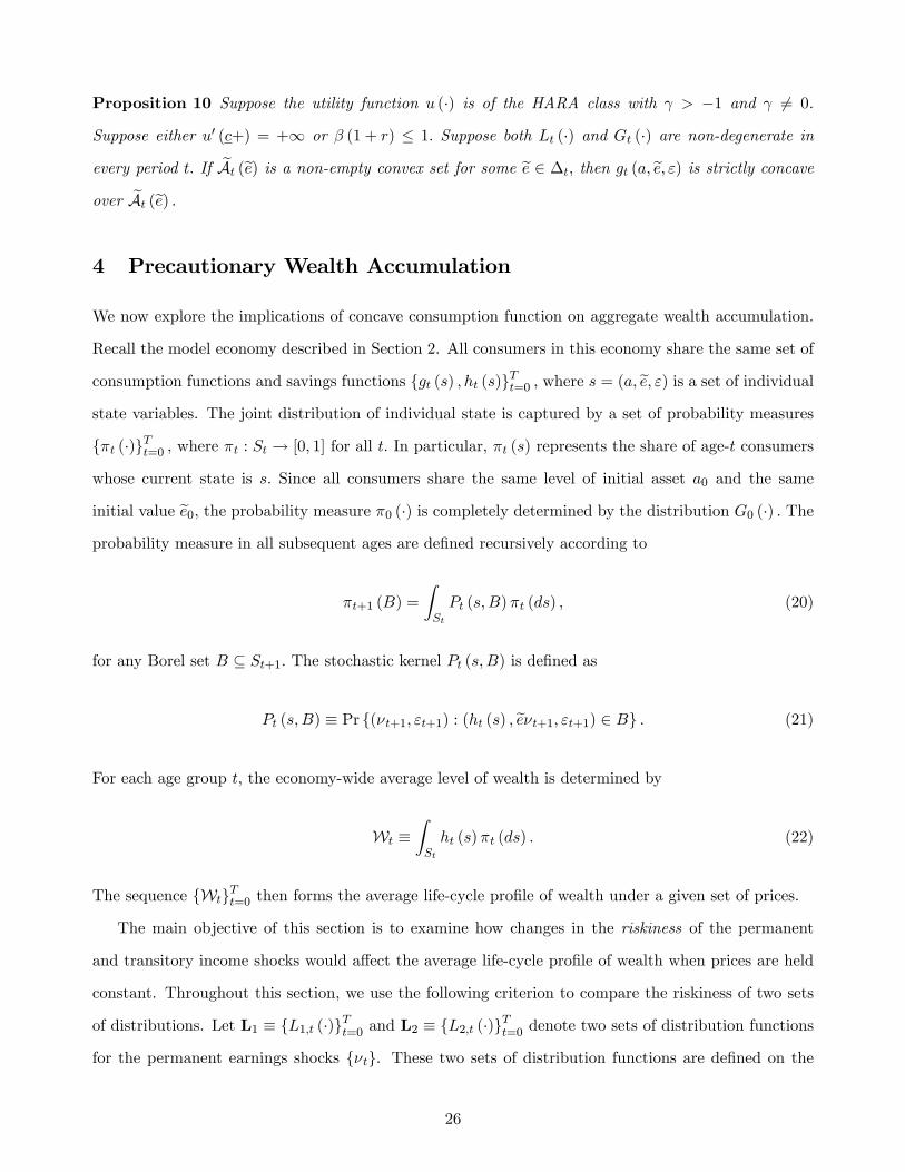
every period t: If eAt (ee) is a non-empty convex set for some ee 2 �t; then gt (a; ee; ") is strictly concaveover eAt (ee) :4 Precautionary Wealth Accumulation

We now explore the implications of concave consumption function on aggregate wealth accumulation.

Recall the model economy described in Section 2. All consumers in this economy share the same set of

consumption functions and savings functions fgt (s) ; ht (s)gTt=0 ; where s = (a; ee; ") is a set of individualstate variables. The joint distribution of individual state is captured by a set of probability measures

f�t (�)gTt=0 ; where �t : St ! [0; 1] for all t: In particular, �t (s) represents the share of age-t consumers

whose current state is s: Since all consumers share the same level of initial asset a0 and the same

initial value ee0; the probability measure �0 (�) is completely determined by the distribution G0 (�) : Theprobability measure in all subsequent ages are de�ned recursively according to

�t+1 (B) =

ZSt

Pt (s;B)�t (ds) ; (20)

for any Borel set B � St+1: The stochastic kernel Pt (s;B) is de�ned as

Pt (s;B) � Pr f(�t+1; "t+1) : (ht (s) ; ee�t+1; "t+1) 2 Bg : (21)

For each age group t; the economy-wide average level of wealth is determined by

Wt �ZSt

ht (s)�t (ds) : (22)

The sequence fWtgTt=0 then forms the average life-cycle pro�le of wealth under a given set of prices.

The main objective of this section is to examine how changes in the riskiness of the permanent

and transitory income shocks would a¤ect the average life-cycle pro�le of wealth when prices are held

constant. Throughout this section, we use the following criterion to compare the riskiness of two sets

of distributions. Let L1 � fL1;t (�)gTt=0 and L2 � fL2;t (�)gTt=0 denote two sets of distribution functions

for the permanent earnings shocks f�tg. These two sets of distribution functions are de�ned on the

26

same compact interval � � [�; �] : The distributions in L1 are said to be more risky than those in L2

if the inequality below holds for all t 2 f0; 1; :::; Tg and for all concave function f : �! R;

Z�f (�) dL1;t (�) �

Z�f (�) dL2;t (�) ;

provided that the integrals exist. As shown in Rothschild and Stiglitz (1970), this de�nition is equivalent

to saying that each L1;t (�) is a mean-preserving spread of L2;t (�) : It also means that the variance of

L1;t (�) is no less than that of L2;t (�) in every period t. The same criterion is also used to compare the

riskiness of any two sets of distributions for the transitory earnings shocks f"tg :

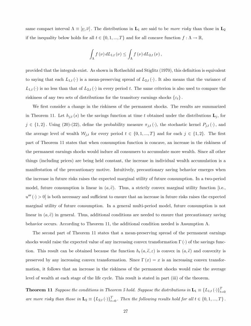
We �rst consider a change in the riskiness of the permanent shocks. The results are summarized

in Theorem 11. Let hj;t (s) be the savings function at time t obtained under the distributions Lj ; for

j 2 f1; 2g : Using (20)-(22), de�ne the probability measure �j;t (�), the stochastic kernel Pj;t (�) ; and

the average level of wealth Wj;t for every period t 2 f0; 1; :::; Tg and for each j 2 f1; 2g. The �rst

part of Theorem 11 states that when consumption function is concave, an increase in the riskiness of

the permanent earnings shocks would induce all consumers to accumulate more wealth. Since all other

things (including prices) are being held constant, the increase in individual wealth accumulation is a

manifestation of the precautionary motive. Intuitively, precautionary saving behavior emerges when

the increase in future risks raises the expected marginal utility of future consumption. In a two-period

model, future consumption is linear in (a; ee). Thus, a strictly convex marginal utility function [i.e.,u000 (�) > 0] is both necessary and su¢ cient to ensure that an increase in future risks raises the expected

marginal utility of future consumption. In a general multi-period model, future consumption is not

linear in (a; ee) in general. Thus, additional conditions are needed to ensure that precautionary savingbehavior occurs. According to Theorem 11, the additional condition needed is Assumption A.

The second part of Theorem 11 states that a mean-preserving spread of the permanent earnings

shocks would raise the expected value of any increasing convex transformation � (�) of the savings func-

tion. This result can be obtained because the function ht (a; ee; ") is convex in (a; ee) and convexity ispreserved by any increasing convex transformation. Since � (x) = x is an increasing convex transfor-

mation, it follows that an increase in the riskiness of the permanent shocks would raise the average

level of wealth at each stage of the life cycle. This result is stated in part (iii) of the theorem.

Theorem 11 Suppose the conditions in Theorem 5 hold. Suppose the distributions in L1 � fL1;t (�)gTt=0are more risky than those in L2 � fL2;t (�)gTt=0 : Then the following results hold for all t 2 f0; 1; :::; Tg :

27

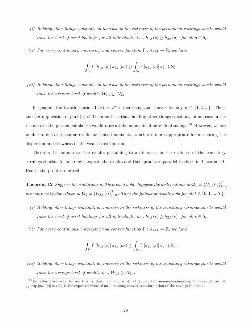
(i) Holding other things constant, an increase in the riskiness of the permanent earnings shocks would

raise the level of asset holdings for all individuals, i.e., h1;t (s) � h2;t (s) ; for all s 2 St:

(ii) For every continuous, increasing and convex function � : At+1 ! R; we have

ZSt

� [h1;t (s)]�1;t (ds) �ZSt

� [h2;t (s)]�2;t (ds) :

(iii) Holding other things constant, an increase in the riskiness of the permanent earnings shocks would

raise the average level of wealth, W1;t � W2;t:

In general, the transformation � (x) = xn is increasing and convex for any n 2 f1; 2; :::g : Thus,

another implication of part (ii) of Theorem 11 is that, holding other things constant, an increase in the

riskiness of the permanent shocks would raise all the moments of individual savings.29 However, we are

unable to derive the same result for central moments, which are more appropriate for measuring the

dispersion and skewness of the wealth distribution.

Theorem 12 summarizes the results pertaining to an increase in the riskiness of the transitory

earnings shocks. As one might expect, the results and their proof are parallel to those in Theorem 11.

Hence, the proof is omitted.

Theorem 12 Suppose the conditions in Theorem 5 hold. Suppose the distributions inG1 � fG1;t (�)gTt=0are more risky than those in G2 � fG2;t (�)gTt=0 : Then the following results hold for all t 2 f0; 1; :::; Tg :

(i) Holding other things constant, an increase in the riskiness of the transitory earnings shocks would

raise the level of asset holdings for all individuals, i.e., h1;t (s) � h2;t (s) ; for all s 2 St:

(ii) For every continuous, increasing and convex function � : At+1 ! R; we have

ZSt

� [h1;t (s)]�1;t (ds) �ZSt

� [h2;t (s)]�2;t (ds) :

(iii) Holding other things constant, an increase in the riskiness of the transitory earnings shocks would

raise the average level of wealth, i.e., W1;t � W2;t:

29An alternative way to see this is that, for any n 2 f1; 2; :::g ; the moment-generating function M (n) �RStexp [nht (s)]�t (ds) is the expected value of an increasing convex transformation of the savings function.

28

5 Numerical Examples

In this section, we provide a set of numerical examples in which the utility function has strictly positive

third derivative, but the inverse of absolute prudence I (c) � �u00 (c) =u000 (c) is not a globally concave

function. Under certain parameter values, the consumption function in certain period is not globally

concave in either (a; ee) or (a; ") : These examples thus illustrate the importance of the concavity of I (�)in Theorem 5. Using the non-concave consumption functions, we then construct examples in which a

mean-preserving spread in the transitory earnings shock would lead to a reduction in aggregate savings.

These results illustrate the importance of the concavity of I (�) in Theorem 12.

Suppose now the consumers live only three periods, i.e., T = 2: Each consumer solves the optimiza-

tion problem described in Section 2. The borrowing limits at are equal to zero in all three periods. In

both the second and third periods, the permanent shock �t is drawn from a �nite set f�1; :::; �Jg with

probabilities fp1; :::; pJg : In the existing literature, it is typical to assume that �t is i.i.d. over time

and has a lognormal distribution with mean zero and variance �2� : Thus, we choose the elements in

f�1; :::; �Jg and fp1; :::; pJg so as to approximate such a distribution. First, we truncate a lognormal

distribution with mean zero and variance �2� by discarding the top 0.5% and the bottom 0.5%. Then,

we divide the restricted domain into J evenly-spaced intervals. The probability pj is the probability of

drawing �t from the jth interval, and �j is the mid-point of that interval. We set J = 50: The value of

�2� is chosen so that the variance of ln �t from the discrete distribution is 0.0212, which is consistent with

the estimate obtained by Gourinchas and Parker (2002). After �t is drawn, the permanent componenteet is updated according to eet = eet�1�t; with ee0 = 1:As for the transitory earnings shock, we assume that "t take only two possible values, f1� {t; 1 + {tg ;

with equal probability in all three periods. We adopt this speci�cation because a mean-preserving spread

in "t can be obtained simply by increasing {t: In the benchmark example, we set {t = 0:1 for all t: To

examine the e¤ects of a mean-preserving spread in the transitory shock, we increase the value of {0,

while maintaining {1 = {2 = 0:1:

The main component of this exercise is the utility function u (�), which is assumed to take the form

u (c) =c1��

1� � +c1��

1� � ; with � > 0 and � > 0: (23)

This function is thrice continuously di¤erentiable and has strictly positive third derivative. Figure 1

29

shows the inverse of absolute prudence I (�) implied by this utility function when � = 10 and � = 0:1:

The function I (�) is convex when the values of consumption are small and concave when the values of

consumption are large. Similar pattern can be obtained for a wide range of values of � and �: Huggett

and Vidon (2002) consider the sum of two exponential utility functions, i.e.,

u (c) = � 1�exp (��c)� 1

�exp (��c) ; with � > 0 and � > 0; (24)

which also yields a convex-concave form of I (�) when the di¤erence between � and � is large. These

two speci�cations, however, have very di¤erent implications for the relative risk aversion. For the one

Table 1: Results on Asset Holdings

{0 = 0:10 {0 = 0:25 {0 = 0:50 {0 = 0:75

Optimal Savings at t = 0

h0 (a0; ee0; 1� {0) 1.5222 1.5039 1.4683 1.4250

h0 (a0; ee0; 1 + {0) 1.5440 1.5588 1.5818 1.6035

W1 1.5331 1.5314 1.5250 1.5142

Optimal Savings at t = 1

E (a2j"0 = 1� {0) 0.7249 0.7192 0.7076 0.6928

E (a2j"0 = 1 + {0) 0.7315 0.7359 0.7425 0.7485

W2 0.7282 0.7275 0.7251 0.7207

in (23), the coe¢ cient of relative risk aversion decreases monotonically from 10 to 0.1 as c increases.

For the utility function in (24), the relative risk aversion is a non-monotonic function in consumption.

The other parameter values that we used are � = 0:9; r = 0:03; w = 0:5, and a0 = 2:6:

To derive the consumption functions in the �rst and second periods, we solve the Euler equation on

a set of 2,501 evenly-spaced gridpoints for current asset holdings over the interval [0; 2:5] : Figure 2 plots

the consumption function g1 (a; ee; ") under various combinations of ee1 and "1: In the diagram, Case 1corresponds to the pair (ee1; "1) = (0:6825; 0:9) ; Case 2 corresponds to the pair (ee1; "1) = (0:9178; 1:1),and Case 3 corresponds to (ee1; "1) = (1:2537; 1:1) : It is clear that the consumption function is convexunder certain range of asset values. Since g1 (a; ee; ") is locally convex in a for some (ee; ") ; it cannot beglobally concave in (a; ee) or in (a; ") :

Next, we consider the e¤ects of increasing {0 when all other parameters (including {1 and {2) are

30

held constant. The results are summarized in Table 1. Under the benchmark speci�cation, an increase

in {0 would lower the unconditional expectation of a1 and a2; represented by W1 and W2; respectively.

The intuitions of this result are as follows. Since the savings function in the �rst period is increasing in

"0, an increase in {0 reduces savings when "0 = 1�{0 [i.e., h0 (a0; ee0; 1� {0)] and raises savings when"0 = 1+{0 [i.e., h0 (a0; ee0; 1 + {0)]. This essentially widens the dispersion of asset holdings in the secondperiod. In addition, the decline in h0 (a0; ee0; 1� {0) is larger than the increase in h0 (a0; ee0; 1 + {0)in all cases. Thus, the unconditional expectation W1 falls as {0 increases. As for the second period,

let E (a2j"0 = 1� {0) and E (a2j"0 = 1 + {0) be the expectations of a2 = h1 (a1; ee1; "1) conditionalon the realization of "0: Table 1 shows that an increase in {0 also widens the dispersion of these

conditional expectations. In particular, the decline in E (a2j"0 = 1� {0) is larger than the increase in

E (a2j"0 = 1 + {0) : This is due to two factors. First, the consumption function g1 (a1; ee1; "1) exhibitslocal convexity, as depicted in Figure 2. This means the savings function h1 (a1; ee1; "1) is locally concave.Second, an increase in {0 widens the dispersion of h0 (a0; ee0; "0) : These in turn lead to a reduction inthe unconditional expectation W2 as {0 increases.

6 Concluding Remarks

In this paper, we explore the theoretical foundations for the concavity of consumption function and

precautionary wealth accumulation. This study departs from the existing literature by considering a

general class of utility functions. We show that the consumption function at each stage of the life cycle

exhibits concavity when the utility function has strictly positive third derivative and the inverse of

absolute prudence is a concave function. We also show that when consumption function is concave,

a mean-preserving spread in either permanent or transitory earnings shock would encourage wealth

accumulation at both the individual and aggregate levels. Finally, our numerical examples show that if

the inverse of absolute prudence is not globally concave, then the consumption function may be locally

convex and precautionary saving may not occur even when the utility function has strictly positive

third derivative.

31

Figure 1: Inverse of Absolute Prudence when � = 10 and � = 0:1:

Figure 2: Consumption Functions in the Second Period.

32

Appendix A

Proof of Theorem 1

The proof of this theorem is divided into two parts. The �rst part establishes the boundedness and the

continuity of the value functions. Once these properties are established, the proofs of strict monotonicity

and strict concavity are standard and are thus omitted. The second part of the proof establishes the

di¤erentiability of Vt (�; z) for each t and for all z 2 Zt: An inductive argument is used in each part.

For each t 2 f0; 1; :::; Tg ; de�ne dt � wet � (1 + r) at + at+1:

Part 1: Boundedness and Continuity

In the terminal period, the value function is given by

VT (a; z) = u [we (z) + (1 + r) a] ; for all (a; z) 2 ST :

This function is bounded above by u [weT + (1 + r) aT ] <1; bounded below by

u [weT � (1 + r) aT ] > u (c) � �1; (25)

and continuous on ST : The �rst inequality in (25) follows from condition (3).

Suppose Vt+1 (a; z) is bounded and continuous on St+1 for some t + 1 � T: For each (a; z) 2 St;

de�ne the budget correspondence Bt according to

Bt (a; z) ��c : c � c � x (a; z) + at+1

;

where x (a; z) � we (z) + (1 + r) a: De�ne the objective function at time t as

Wt (c; a; z) � u (c) + �

ZZt+1

Vt+1�x (a; z)� c; z0

�Qt�z; dz0

�:

Since Vt+1 (a; z) is bounded and continuous on St+1; the conditional expectation in the above expression

is well-de�ned. Since the transition function Qt satis�es the Feller property, Wt is continuous whenever

it is �nite. If u (c) > �1; then the objective functionWt (c; a; z) is bounded and continuous on Bt (a; z)

for all (a; z) 2 St: By the Theorem of the Maximum, the value function Vt is continuous and the optimal

33

policy correspondence gt de�ned in (4) is non-empty, compact-valued and upper hemicontinuous. Since

Wt (c; a; z) is bounded for all c 2 Bt (a; z) and for all (a; z) 2 St; the value function Vt (�) is also bounded.

Suppose now u (c) = �1: In this case, Wt (c; a; z) = �1 for all (a; z) 2 St: This means for all

(a; z) 2 St; the objective function in (P1) is not continuous on the budget set. Consequently, we cannot

apply the Theorem of the Maximum directly. However, the same results can be obtained with some

additional e¤ort. The following argument is similar to the one used in Alvarez and Stokey (1998)

Lemma 2. Given (3), we have x (a; z)+ at+1 � dt > c; for all (a; z) 2 St and for all t: De�ne a modi�ed

budget correspondence B�t according to

B�t (a; z) ��c : dt � c � x (a; z) + at+1

:

This correspondence is non-empty, compact-valued and continuous. Most importantly, the objective

function Wt (c; a; z) is �nite and continuous on B�t (a; z) for all (a; z) 2 St: De�ne the set of maximizers

of Wt (c; a; z) on B�t (a; z) as

g�t (a; z) � argmaxc2B�t (a;z)

fWt (c; a; z)g :

Then g�t (a; z) is non-empty and Wt (c�; a; z) > �1 for any c� 2 g�t (a; z) : Pick any c

� 2 g�t (a; z) :

If Wt (c�; a; z) � Wt (c; a; z) for all c 2 [c; dt) ; then c� 2 gt (a; z) : Suppose there exists ec 2 [c; dt)

such that Wt (ec; a; z) > Wt (c�; a; z) > �1, then ec 2 gt (a; z) : In either case, the optimal policy

correspondence gt (a; z) is non-empty. Note that in the latter case, ec must be strictly greater than cbecause Wt (ec; a; z) > �1: It follows that c > c whenever c 2 gt (a; z) : Hence Vt (a; z) > �1: Since

Wt (c; a; z) is still bounded above for all c 2 Bt (a; z) and for (a; z) 2 St; the value function Vt (�) is also

bounded above.

We now establish the continuity of Vt (�) for the case when u (c) = �1: Since Vt (�) is single-valued,

it su¢ ce to show that it is upper hemicontinuous. Let f(an; zn)g be a sequence in St that converges

to some (a; z) 2 St: Pick a sequence of consumption fcng such that cn 2 gt (an; zn) for each n: Such

a sequence can always be drawn because gt (an; zn) is non-empty for all n: Since cn 2 Bt (an; zn)

and Bt is compact-valued and upper hemicontinuous, there exists a subsequence of fcng ; denoted

by fcnkg ; such that cnk converges to some c�� 2 Bt (a; z) : Since cnk 2 gt (ank ; znk) ; it follows that

cnk > c and Wt (cnk ; ank ; znk) > �1 for all nk: By the continuity of Wt (�) ; we have Vt (ank ; znk) =

Wt (cnk ; ank ; znk) ! Wt (c��; a; z) : If we can show that Wt (c

��; a; z) = Vt (a; z) ; then this will estab-

34

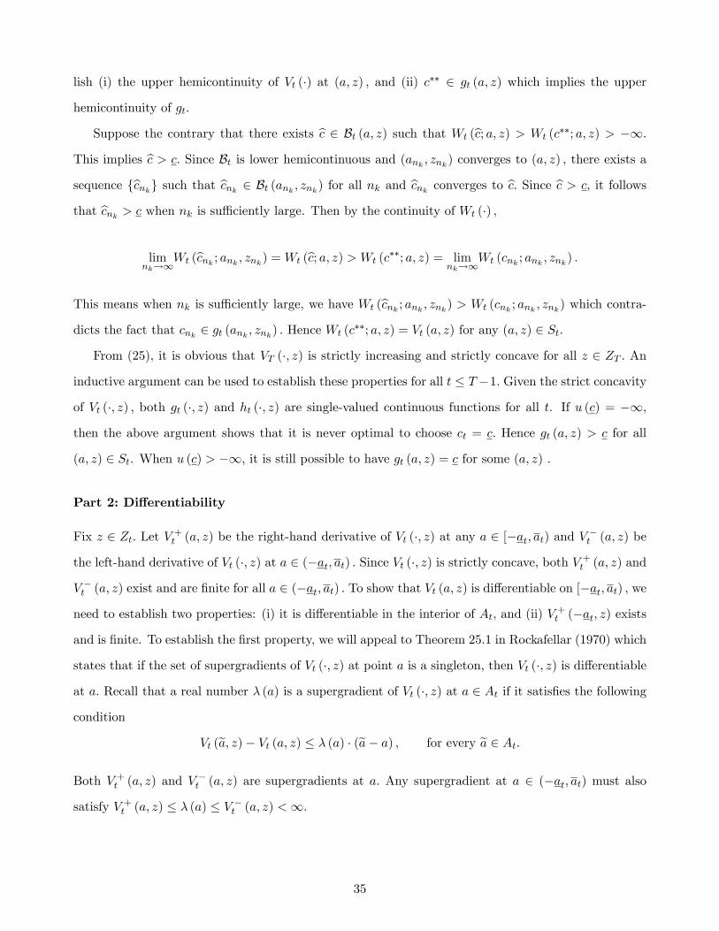
lish (i) the upper hemicontinuity of Vt (�) at (a; z) ; and (ii) c�� 2 gt (a; z) which implies the upper

hemicontinuity of gt:

Suppose the contrary that there exists bc 2 Bt (a; z) such that Wt (bc; a; z) > Wt (c��; a; z) > �1:

This implies bc > c: Since Bt is lower hemicontinuous and (ank ; znk) converges to (a; z) ; there exists a

sequence fbcnkg such that bcnk 2 Bt (ank ; znk) for all nk and bcnk converges to bc: Since bc > c; it follows

that bcnk > c when nk is su¢ ciently large. Then by the continuity of Wt (�) ;

limnk!1

Wt (bcnk ; ank ; znk) =Wt (bc; a; z) > Wt (c��; a; z) = lim

nk!1Wt (cnk ; ank ; znk) :

This means when nk is su¢ ciently large, we have Wt (bcnk ; ank ; znk) > Wt (cnk ; ank ; znk) which contra-

dicts the fact that cnk 2 gt (ank ; znk) : Hence Wt (c��; a; z) = Vt (a; z) for any (a; z) 2 St:

From (25), it is obvious that VT (�; z) is strictly increasing and strictly concave for all z 2 ZT : An

inductive argument can be used to establish these properties for all t � T�1: Given the strict concavity

of Vt (�; z) ; both gt (�; z) and ht (�; z) are single-valued continuous functions for all t. If u (c) = �1;

then the above argument shows that it is never optimal to choose ct = c: Hence gt (a; z) > c for all

(a; z) 2 St. When u (c) > �1; it is still possible to have gt (a; z) = c for some (a; z) :

Part 2: Di¤erentiability

Fix z 2 Zt: Let V +t (a; z) be the right-hand derivative of Vt (�; z) at any a 2 [�at; at) and V �t (a; z) be

the left-hand derivative of Vt (�; z) at a 2 (�at; at) : Since Vt (�; z) is strictly concave, both V +t (a; z) and

V �t (a; z) exist and are �nite for all a 2 (�at; at) : To show that Vt (a; z) is di¤erentiable on [�at; at) ; we

need to establish two properties: (i) it is di¤erentiable in the interior of At; and (ii) V +t (�at; z) exists

and is �nite. To establish the �rst property, we will appeal to Theorem 25.1 in Rockafellar (1970) which

states that if the set of supergradients of Vt (�; z) at point a is a singleton, then Vt (�; z) is di¤erentiable

at a: Recall that a real number � (a) is a supergradient of Vt (�; z) at a 2 At if it satis�es the following

condition

Vt (ea; z)� Vt (a; z) � � (a) � (ea� a) ; for every ea 2 At:Both V +t (a; z) and V

�t (a; z) are supergradients at a: Any supergradient at a 2 (�at; at) must also

satisfy V +t (a; z) � � (a) � V �t (a; z) <1:

35

An inductive argument is used in the following proof. In the terminal period, we have

gT (a; z) = we (z) + (1 + r) a � dT > c;

and VT (a; z) = u [we (z) + (1 + r) a] ; for all (a; z) 2 ST : Under the stated assumptions for u (�) ;

VT (�; z) is continuously di¤erentiable in the interior of AT and the derivative is given by pT (a; z) =

(1 + r)u0 [gT (a; z)] : Also, the right-hand derivative of VT (�; z) at a = �aT exists and is given by

(1 + r)u0 [gT (�aT ; z)] which is �nite. Suppose the desired result is true for some t + 1 � T and

gt+1 (a0; z0) > c for all (a0; z0) 2 St+1: The remaining proof is divided into several steps. Steps 1-4

essentially establish all the results in Theorem 2.

Step 1 First, we show that if gt (a; z) > c; then gt (a; z) and ht (a; z) satis�es

u0 [gt (a; z)] � �

ZZt+1

pt+1�ht (a; z) ; z

0�Qt �z; dz0� : (26)

If in addition ht (a; z) > �at+1; then (26) holds with equality.

Fix (a; z) 2 St: De�ne ec = gt (a; z) and ea0 = ht (a; z) : If ec > c; then ea0 < at+1: Suppose now we

increase ea0 by � > 0; reduce ec by � > 0 but maintain ec � � > c: The utility loss generated by this is

u (ec)� u (ec� �) : The utility gain generated by this is�

ZZt+1

�Vt+1

�ea0 + �; z0�� Vt+1 �ea0; z0��Qt �z; dz0� :If the borrowing constraint is binding originally, i.e., ea0 = �at+1, then any reduction in consumptionwould lower the value of the objective function. This means the loss in utility is no less than the gain

so thatu (ec)� u (ec� �)

�� �

ZZt+1

�Vt+1 (ea0 + �; z0)� Vt+1 (ea0; z0)

�

�Qt�z; dz0

�:

By taking the limit �! 0+; we get

u0 (ec) � lim�!0+

(�

ZZt+1

�Vt+1 (ea0 + �; z0)� Vt+1 (ea0; z0)

�

�Qt�z; dz0

�): (27)

36

Since Vt+1 (a0; z0) is strictly concave in a0; the function

��;ea0; z0� � Vt+1 (ea0 + �; z0)� Vt+1 (ea0; z0)

�> 0

is strictly decreasing in �: Hence, it is bounded above by pt+1 (ea0; z0) which is �nite as Vt+1 (�; z0)is di¤erentiable on

��at+1; at+1

�. By the Lebesgue Convergence Theorem, the limit in (27) can be

expressed as

�

ZZt+1

lim�!0+

�Vt+1 (ea0 + �; z0)� Vt+1 (ea0; z0)

�

�Qt�z; dz0

�= �

ZZt+1

pt+1�ea0; z0�Qt �z; dz0� :

Substituting this into (27) gives (26) for the case when ea0 = ht (a; z) = �at+1: If ea0 = ht (a; z) > �at+1;

then any in�nitesimal change in consumption would not a¤ect the maximized value of the objective.

This means (27) will hold with equality. It follows from the above argument that (26) holds with

equality when ea0 = ht (a; z) > �at+1:

Step 2 Using a similar perturbation argument, we can show that if gt (a; z) = c; then the following

condition must be satis�ed

u0 (c+) � �

ZZt+1

pt+1�ht (a; z) ; z

0�Qt �z; dz0� ; (28)

where u0 (c+) denote the right-hand derivative of u (�) at c: Suppose ec = gt (a; z) = c for some (a; z) 2 St:

Suppose now we increase ec by � > 0, reduce ea0 = ht (a; z) by � > 0; but maintain ea0 � � � �at+1: If it

is optimal to consume c; then any in�nitesimal increase in consumption would either lower or have no

e¤ect on the value of the objective function. Hence,

lim�!0+

�u (c+ �)� u (c)

�

�= u0 (c+) � �

ZZt+1

lim�!0+

�Vt+1 (ea0; z0)� Vt+1 (ea0 � �; z0)

�

�Qt�z; dz0

�:

Since Vt+1 (�; z0) is di¤erentiable on��at+1; at+1

�; the left-hand derivative in the above expression exists

and is given by pt+1 [ht (a; z) ; z0] :

Step 3 We now show that gt (a; z) > c if either u0 (c+) = +1 or � (1 + r) � 1 holds. If u0 (c+) = +1,

then (28) cannot be satis�ed and hence it is never optimal to consume the minimum level c: Consider

the case when u0 (c+) < +1 and � (1 + r) � 1: By the induction hypothesis, we have gt+1 (a0; z0) > c

37

and pt+1 (a0; z0) = (1 + r)u0 [gt+1 (a0; z0)] for all (a0; z0) 2 St+1: Fix (a; z) 2 St: Suppose the contrary

that gt (a; z) = c: Then according to Step 2, it must be the case that

u0 (c+) � � (1 + r)

ZZt+1

u0�gt+1

�ht (a; z) ; z

0��Qt �z; dz0��

ZZt+1

u0�gt+1

�ht (a; z) ; z

0��Qt �z; dz0�< u0 (c+) :

The second inequality uses the assumption that � (1 + r) � 1: The third inequality uses the fact that

gt+1 (a0; z0) > c for all (a0; z0) 2 St+1: This gives rise to a contradiction. Hence gt (a; z) > c for all

(a; z) 2 St: This means the optimal policy functions would only satisfy (26), but not (28).

Step 4 We now show that gt (a; ee; ") is strictly increasing for all (a; ee; ") 2 St: This is true for

gT (a; ee; ") : Suppose gt+1 (a0; ee0; "0) is strictly increasing for all (a0; ee0; "0) 2 St+1: Pick any (a2; ee2; "2)and (a1; ee1; "1) from St such that a2 � a1; ee2 � ee1 and "2 � "1 with strict inequality holds for at least

one variable. Suppose the contrary that gt (a2; ee2; "2) � gt (a1; ee1; "1) ; which implies ht (a2; ee2; "2) >ht (a1; ee1; "1) � �at+1: Since gt+1 (a0; ee0; "0) is strictly increasing, we have

gt+1�ht (a2; ee2; "2) ; ee2� 0; "0� > gt+1

�ht (a1; ee1; "2) ; ee1� 0; "0�

) u0�gt+1

�ht (a2; ee2; "2) ; ee2� 0; "0�� < u0

�gt+1

�ht (a1; ee1; "2) ; ee1� 0; "0�� ;

for all (� 0; "0) 2 �� �: Integrating this over all possible values of (� 0; "0) gives

u0 [gt (a2; ee2; "2)] = � (1 + r)

Z�

Z�u0�gt+1

�ht (a2; ee2; "2) ; ee2� 0; "0�� dLt+1 �� 0� dGt+1 �"0�

< � (1 + r)

Z�

Z�u0�gt+1

�ht (a1; ee1; "1) ; ee1� 0; "0�� dLt+1 �� 0� dGt+1 �"0�

� u0 [gt (a1; ee1; "1)] :The �rst line uses the Euler equation and the fact that ht (a2; ee2; "2) > �at+1: The above result

contradicts gt (a2; ee2; "2) � gt (a1; ee1; "1) : Hence gt (a; ee; ") is a strictly increasing function. A similar

argument can be used to show that, for any given ee 2 �t; the savings function ht (a; ee; ") is nondecreasingin (a; ") :

38

Step 5 We now show that Vt (�; z) is di¤erentiable in the interior of At and pt (�; z) = (1+r)u0 [gt (�; z)]

for each z 2 Zt: Fix z 2 Zt: Let �t (a; z) be a supergradient of Vt (a; z) at a 2 (�at; at) : Since Vt (�; z)

is strictly increasing and strictly concave on At, �t (a; z) is strictly positive and �nite: The main idea

of the proof is to show that for any a 2 (�at; at) ; there exists a neighborhoodM (a; z) of gt (a; z) such

that gt (a; z) is an interior solution of the following problem

maxc2M(a;z)

f(1 + r)u (c)� �t (a; z) cg : (P4)

This problem is well-posed as �t (a; z) is �nite and the objective function is strictly concave. If gt (a; z)

is an interior solution of (P4), then it must satisfy the �rst-order condition

�t (a; z) = (1 + r)u0 [gt (a; z)] :

Since this is true for any supergradient �t (a; z) ; this means (1 + r)u0 [gt (a; z)] must be the unique

supergradient at a 2 (�at; at) and so Vt (�; z) is di¤erentiable at a: We now establish the key steps of

this argument. Fix a 2 (�at; at) : Since gt (a; z) > c � 0 and (1 + r) > 0; we can �nd an � > 0 such

that

a� � � max��at; a�

gt (a; z)� c1 + r

�and a+ � < at:

For any ea 2 (a� �; a+ �) ; de�ne c (ea) according toc (ea) = we (z) + (1 + r)ea� ht (a; z) = (1 + r) (ea� a) + gt (a; z) : (29)

which is strictly greater than c as ea > a�� � a�[gt (a; z)� c] = (1 + r) : In other words, the combination

of c (ea) and ht (a; z) is feasible when the current state is (ea; z) : In addition, ea 2 (a� �; a+ �) impliesc (ea) is within a certain neighborhood of gt (a; z) given by

M� (a; z) = fc : gt (a; z)� (1 + r) � < c < gt (a; z) + (1 + r) �g :

The rest of the proof is similar to the proof of Lemma 1.1 in Schechtman (1976). Let �t (a; z) be a

supergradient of Vt (a; z) at a 2 (�at; at) : Then for any ea 2 At; we haveVt (ea; z)� Vt (a; z) � �t (a; z) � (ea� a) :

39

Since �t (a; z) is �nite, we can rewrite this as

Vt (ea; z)� �t (a; z)ea � Vt (a; z)� �t (a; z) a: (30)

This inequality has to be true for any ea 2 At: So pick ea 2 (a� �; a+ �) and de�ne c (ea) as in (29).Since c (ea) and ht (a; z) are feasible when the current state is (ea; z) ; it follows from the de�nition of the

value function and (30) that

u [c (ea)] + � ZZt+1

Vt+1�ht (a; z) ; z

0�Qt �z; dz0�� �t (a; z) � �ht (a; z) + c (ea)� we (z)1 + r

�� Vt (ea; z)� �t (a; z) � �ht (a; z) + c (ea)� we (z)

1 + r

�� Vt (a; z)� �t (a; z) �

�ht (a; z) + gt (a; z)� we (z)

1 + r

�= u [gt (a; z)] + �

ZZt+1

Vt+1�ht (a; z) ; z

0�Qt �z; dz0�� �t (a; z) � �ht (a; z) + gt (a; z)� we (z)1 + r

�:

This can be simpli�ed to become

(1 + r)u [c (ea)]� �t (a; z) c (ea) � (1 + r)u [gt (a; z)]� �t (a; z) gt (a; z) ;which is true for all c (ea) 2 M� (a; z). In other words, gt (a; z) is an interior solution of the problem

(P4). This establishes the desired results.

Step 6 We now show that Vt (a; z) is right-hand di¤erentiable at a = �at and the right-hand derivative

is given by (1 + r)u0 [gt (�at; z)] : Fix z 2 Zt and a 2 (�at; at) : By the concavity of u (�) ; we have

u [gt (a; z)]� u [gt (�at; z)] � u0 [gt (�at; z)] [gt (a; z)� gt (�at; z)] :

The result in Step 3 implies u0 [gt (�at; z)] < u0 (c) � +1: Similarly, by the concavity and di¤erentia-

bility of Vt+1 (�; z0) on��at+1; at+1

�; we have

Vt+1�ht (a; z) ; z

0�� Vt+1(ht (�at; z) ; z0) � pt+1�ht (�at; z) ; z0

�� [ht (a; z)� ht (�at; z)] ;

40

for all z0 2 Zt+1: Using these, we can write

Vt (a; z)� Vt (�at; z)

= u [gt (a; z)]� u [gt (�at; z)]

+�

ZZt+1

�Vt+1

�ht (a; z) ; z

0�� Vt+1(ht (�at; z) ; z0)�Qt �z; dz0�� u0 [gt (�at; z)] [gt (a; z)� gt (�at; z)]

+�

"ZZt+1

pt+1�ht (�at; z) ; z0

�Qt�z; dz0

�#[ht (a; z)� ht (�at; z)]

� u0 [gt (�at; z)] [gt (a; z) + ht (a; z)� gt (�at; z)� ht (�at; z)] = u0 [gt (�at; z)] (1 + r) (a+ at) :

The second line follows from the de�nition of Vt (a; z) and Vt (�at; z) : The fourth line is obtained

by using condition (26) and the fact that ht (a; z) is non-decreasing in a: The last equality uses the

consumer�s budget constraint. Thus, we have

Vt (a; z)� Vt (�at; z)a� (�at)

� (1 + r)u0 [gt (�at; z)] < +1:

By taking the limit a ! �at+; we can establish that V +t (�at; z) exists and is bounded above by

(1 + r)u0 [gt (�at; z)] : Hence V +t (�at; z) is �nite. Since V +t (a; z) is strictly decreasing in a, we have

(1 + r)u0 [gt (a; z)] = V +t (a; z) < V +t (�at; z) � (1 + r)u0 [gt (�at; z)] ;

for all a 2 (�at; at) : Since both u0 (c) and gt (�; z) are continuous, we have u0 [gt (a; z)]! u0 [gt (�at; z)]

as a! �at: Hence V +t (�at; z) = (1 + r)u0 [gt (�at; z)] : This completes the proof of Theorem 1.

Proof of Theorem 2

Part (i) of this theorem is proved in Step 3 of the second part of the above proof. Part (ii) of Theorem

2 is established in Step 1 of that proof. Part (iii) is established in Step 4 of that proof.

Proof of Theorem 3

For each z 2 Zt and for each t 2 f0; 1; :::; Tg ; let Ht (z;u) be the hypograph of the policy function

gt (�; z;u) : Formally, Ht (z;u) � f(c; a) 2 D �At : c � gt (a; z;u)g : Using the same step as in the proof

41

of Theorem 5, we can express Ht (z;u) as

Ht (z;u) � f(c; a) 2 D �At : c 2 Bt (a; z) and c � t+1 (x (a; z)� c; z)g ;

where Bt (a; z) is the budget set at state (a; z) in period t; and

t+1�a0; z

�� ��1

(� (1 + r)

ZZt+1

��gt+1

�a0; z0;u

��Qt�z; dz0

�); (31)

for t 2 f0; 1; :::; T � 1g ; with � (c) � u0 (c) : Similarly, de�ne the function

�t+1�a0; z

�� '�1

(� (1 + r)

ZZt+1

'�gt+1

�a0; z0; v

��Qt�z; dz0

�);

for each t 2 f0; 1; :::; T � 1g ; with ' (c) � v0 (c) : Then the hypograph of gt (�; z; v) is given by

Ht (z; v) � f(c; a) 2 D �At : c 2 Bt (a; z) and c � �t+1 (x (a; z)� c; z)g :

Suppose the following inequality holds for all z 2 Z;

�t+1 (�; z) � t+1 (�; z) : (32)

Then we have Ht (z; v) � Ht (z;u) for all z 2 Z; and it follows that gt (a; z; v) � gt (a; z;u) for all

(a; z) 2 St: Hence, it su¢ ce to show that (32) holds for all z 2 Zt and t 2 f0; 1; :::; T � 1g : This is

achieved in two steps.

Step 1 We �rst derive two useful properties of �(�) : Since �(�) is convex and �(0) � 0; we have

�(�m) � ��(m) for any m � 0 and � 2 [0; 1] : Let m1 and m2 be two strictly positive real numbers

such that m1 > m2 > 0: Then there exists � 2 (0; 1) such that m2 = �m1: Hence,

�(m2) = � (�m1) � ��(m1) =m2

m1�(m1)

) �(m2)

m2� �(m1)

m1:

42

This means m�1�(m) is a nondecreasing function in m > 0: If �(�) is strictly convex, then m�1�(m)

is a strictly increasing function in m > 0: Next, de�ne m � � (c) > 0 for any c 2 D: Substituting

c = ��1 (m) into ' (c) � � [� (c)] gives

'���1 (m)

�= �(m) : (33)

Step 2 We now use an inductive argument to show that (32) holds for all t 2 f0; 1; :::; T � 1g : In the

terminal period, we have gT (a; z; v) = gT (a; z;u) = we (z) + (1 + r) a for all (a; z) 2 ST : Substituting

this into (31) gives

T�a0; z

�� ��1

�� (1 + r)

ZZT

��gT�a0; z0;u

��QT�1

�z; dz0

��= ��1

�� (1 + r)

ZZT

��gT�a0; z0; v

��QT�1

�z; dz0

��

Using (33), we can get

'�T�a0; z

��= �

�� (1 + r)

ZZT

��gT�a0; z0; v

��QT�1

�z; dz0

��: (34)

Since m�1�(m) is a nondecreasing function in m > 0; and � (1 + r) � 1; we have

�n� (1 + r)

RZT� [gT (a

0; z0; v)]QT�1 (z; dz0)o

� (1 + r)RZT� [gT (a0; z0; v)]QT�1 (z; dz0)

��nR

ZT� [gT (a

0; z0; v)]QT�1 (z; dz0)o

RZT� [gT (a0; z0; v)]QT�1 (z; dz0)

; (35)

which implies

'�T�a0; z

��� � (1 + r)�

�ZZT

��gT�a0; z0; v

��QT�1

�z; dz0

��� � (1 + r)

ZZT

����gT�a0; z0; v

��QT�1

�z; dz0

�= � (1 + r)

ZZT

'�gT�a0; z0; v

��QT�1

�z; dz0

�: (36)

The second line uses Jensen�s inequality. The third line uses the fact that ' (c) � � [� (c)] for any

c 2 D: Since '�1 (�) is nonincreasing, we have

T�a0; z

�� '�1

�� (1 + r)

ZZT

'�gT�a0; z0; v

��QT�1

�z; dz0

��� �T

�a0; z

�:

43

As explained above, this implies gT�1 (a; z; v) � gT�1 (a; z;u) for all (a; z) 2 ST�1: Note that if �(�) is

strictly convex, then strict inequality holds in both (35) and (36). These in turn imply gT�1 (a; z; v) <

gT�1 (a; z;u) for all (a; z) 2 ST�1:

Suppose gt+1 (a; z; v) � gt+1 (a; z;u) for all (a; z) 2 St+1 and for some t+1 � T � 1: Using a similar

argument as in (34)-(36), we can get

t+1�a0; z

�� ��1

(� (1 + r)

ZZt+1

��gt+1

�a0; z0;u

��Qt�z; dz0

�)

� '�1

(� (1 + r)

ZZt+1

'�gt+1

�a0; z0;u

��Qt�z; dz0

�): (37)

What remains is to show that

'�1

(� (1 + r)

ZZt+1

'�gt+1

�a0; z0;u

��Qt�z; dz0

�)

� '�1

(� (1 + r)

ZZt+1

'�gt+1

�a0; z0; v

��Qt�z; dz0

�)� �t+1

�a0; z

�: (38)

By the induction hypothesis, we have gt+1 (a; z; v) � gt+1 (a; z;u) for all (a; z) 2 St+1: Since ' (�) is

nonincreasing and � (1 + r) > 0, we have

� (1 + r)

ZZt+1

'�gt+1

�a0; z0;u

��Qt�z; dz0

�� � (1 + r)

ZZt+1

'�gt+1

�a0; z0; v

��Qt�z; dz0

�:

Since '�1 (�) is also nonincreasing, this implies (38). This establishes (32) for all t 2 f0; 1; :::; T � 1g :

If �(�) is strictly convex, then strict inequality holds in (37). It follows that gt (a; z; v) < gt (a; z;u) for

all (a; z) 2 St: This completes the proof of Theorem 3.

Note that the above argument is valid even if fztg is a deterministic process. Suppose the variable

z follows a deterministic time path fz0; z1; :::; zT g such that e (zt) 2 [et; et] for all t: Then (31) becomes

t+1�a0; zt

�� ��1

�� (1 + r)�

�gt+1

�a0; zt+1;u

��:

The expression for �t+1 (a0; z) can be modi�ed in a similar fashion. Using the same argument, we can

show that �t+1 (�; zt) � t+1 (�; zt) for all t; which implies gt (a; zt; v) � gt (a; zt;u) for all a 2 At and

for all t:

44

Proof of Lemma 4

As mentioned in the text, the inequality in (11) becomes Jensen�s inequality when � (1 + r) = 1: Hence,

Assumption A is satis�ed by any concave function � (�) when � (1 + r) = 1: Consider the case when

� (1 + r) 2 (0; 1) : Since u000 (c) > 0 for all c 2 D; we have � (m) � 0 for all m � 0: This, together with

the concavity of � (�) ; implies � (�m) � �� (m) for all m � 0 and � 2 [0; 1] : Using a similar argument

as in Step 1 of the proof of Theorem 3, one can show that m�1� (m) is a nonincreasing function in

m > 0:

Let N � 1 be a positive integer. Let � be a discrete probability measure with masses (�1; :::; �N )

on a set of points ( 1; :::; N ) 2 RN+ : First consider the case whenPNn=1 �n n = 0: Since i � 0 for all

i; this can only happen when either (i) n = 0 for all n; or (ii) n > 0 for some n but �n = 0: In both

cases, we have

�

"� (1 + r)

NXn=1

�n n

#= �(0) > � (1 + r)

NXn=1

�n� ( n) = � (1 + r) � (0) ;

as � (1 + r) 2 (0; 1) : Hence, Assumption A is satis�ed. Next, consider the case whenPNn=1 �n n > 0:

Since m�1� (m) is a nonincreasing function in m > 0; we have

�h� (1 + r)

PNn=1 �n n

i� (1 + r)

PNn=1 �n n

��hPN

n=1 �n n

iPNn=1 �n n

�PNn=1 �n� ( n)PNn=1 �n n

:

The second inequality follows from the concavity of � (�) : Condition (11) can be obtained by rearranging

terms. This completes the proof of Lemma 4.

Proof of Proposition 9

To establish this result, it su¢ ce to show that t+1 (�) is a strictly concave function for any given

period t: To see this, choose " 2 � such that At (") is non-empty and convex. Suppose the contrary

that gt (a; ee; ") has a linear portion over the set At (") : This means there exists (a1; ee1) and (a2; ee2) inAt (") such that for any � 2 (0; 1) ; we have

gt (a�; ee�; ") = �gt (a1; ee1; ") + (1� �) gt (a2; ee2; ") ; (39)

45

where a� � �a1 + (1� �) a2 and ee� � �ee1 + (1� �) ee2: This implies ht (a�; ee�; ") = �ht (a1; ee1; ") +(1� �)ht (a2; ee2; ") : By the strict concavity of t+1 (�) ; we have

t+1 [ht (a�; ee�; ") ; ee�] > �t+1 [ht (a1; ee1; ") ; ee1] + (1� �)t+1 [ht (a2; ee2; ") ; ee2] :Since At (") is a convex set, we have ht (a�; ee�; ") > �at+1: Thus, the Euler equation holds with strictequality under all three states: (a1; ee1; ") ; (a2; ee2; ") and (a�; ee�; ") : This implies

gt (a�; ee�; ") = t+1 [ht (a�; ee�; ") ; ee�]> �t+1 [ht (a1; ee1; ") ; ee1] + (1� �)t+1 [ht (a2; ee2; ") ; ee2]= �gt (a1; ee1; ") + (1� �) gt (a2; ee2; ") ;

which contradicts (39). Hence, gt (a; ee; ") must be strictly concave over At (") :Suppose u (�) is a HARA utility function with > �1 and 6= 0: Then the marginal utility

function is given by � (c) = ' (�+ c)� 1 ; for some ' > 0; and �+ c > 0 for all c 2 D: Then for any

t 2 f0; 1; :::; T � 1g ; the function t+1 (a0; ee) can be expressed ast+1

�a0; ee� � ��1

�� (1 + r)

Z�

Z���gt+1

�a0; ee� 0; "0�� dLt+1 �� 0� dGt+1 �"0��

= �� +[� (1 + r)]�

�Z�

Z�

�gt+1

�a0; ee� 0; "0��� 1

dLt+1�� 0�dGt+1

�"0���

: (40)

Pick any (a01; ee1) and (a02; ee2) from At+1��t: For any � 2 (0; 1) ; de�ne the convex combination (a�; ee�) :By Theorem 5, we know that gt+1 (a0; ee0; "0) is joint concave in its �rst two arguments when "0 is heldconstant. This, together with the assumption that � (�) is strictly decreasing, gives

��gt+1

�a0�; ee�� 0; "0�� � �

��gt+1

�a01; ee1� 0; "0�+ (1� �) gt+1 �a02; ee2� 0; "0�� ;

for all (� 0; "0) 2 �� �: Since ��1 (�) is also strictly decreasing, we have

t+1�a0�; ee��

� ��1�� (1 + r)

Z�

Z����gt+1

�a01; ee1� 0; "0�+ (1� �) gt+1 �a02; ee2� 0; "0�� dLt+1 �� 0� dGt+1 �"0�� :

46

By Minkowski�s inequality for integrals,30 we can get

�Z�

Z�

��gt+1

�a01; ee1� 0; "0�+ (1� �) gt+1 �a02; ee2� 0; "0��� 1

dLt+1�� 0�dGt+1

�"0���

>

�Z�

Z�

��gt+1

�a01; ee1� 0; "0��� 1

dLt+1�� 0�dGt+1

�"0���

+

�Z�

Z�

�(1� �) gt+1

�a02; ee2� 0; "0��� 1

dLt+1�� 0�dGt+1

�"0���

= �

�Z�

Z�

�gt+1

�a01; ee1� 0; "0��� 1

dLt+1�� 0�dGt+1

�"0���

+(1� �)�Z

�

Z�

�gt+1

�a02; ee2� 0; "0��� 1

dLt+1�� 0�dGt+1

�"0���

:

Multiplying both sides by [� (1 + r)]� = > 0 and combining it with (40) gives

t+1�a0�; ee�� > �t+1

�a01; ee1�+ (1� �)t+1 �a02; ee2� :

This completes the proof of Proposition 9.

Proof of Proposition 10

The proof is almost identical to that of Proposition 9. Hence, we only outline the main ideas of the

proof. First, using the same line of argument as in the proof of Proposition 9, one can show the

following: if t+1 (�; ee) is a strictly concave function for any ee 2 �t, then gt (a; ee; ") must be strictlyconcave over eAt (ee) : As shown in the proof of Proposition 9, the function t+1 (�) is strictly concavewhen the utility function is HARA with > �1 and 6= 0: This implies t+1 (�; ee) is a strictly concavefunction for any ee 2 �t: Hence, the desired result follows.Proof of Theorem 11

Part (i) Start from age T � 1: Suppose the contrary that h2;T�1 (a; ee; ") > h1;T�1 (a; ee; ") � �aT ; forsome (a; ee; ") 2 ST�1: Then for any (� 0; "0) 2 �� �; we have

wee� 0"0 + (1 + r)h2;T�1 (a; ee; ") > wee� 0"0 + (1 + r)h1;T�1 (a; ee; ") :30For a formal statement of Minkowski�s inequality for integrals, see Hardy et al. (1952) p.146.

47

Since � (�) is strictly decreasing, we have

��wee� 0"0 + (1 + r)h2;T�1 (a; ee; ")� < �

�wee� 0"0 + (1 + r)h1;T�1 (a; ee; ")� ; (41)

for all (� 0; "0) : Since � (�) is also strictly convex, the expression � [wee� 0"0 + (1 + r)h2;T�1 (a; ee; ")] isstrictly convex in � 0 when (a; ee; "; "0) are held �xed. This, together with the assumption that L1;T (�) ismore risky than L2;T (�) ; implies

Z���wee� 0"0 + (1 + r)h2;T�1 (a; ee; ")� dL1;T �� 0� > Z

���wee� 0"0 + (1 + r)h2;T�1 (a; ee; ")� dL2;T �� 0� ;

(42)

for any given "0 2 �: Using the Euler equation, we can get

� [g1;T�1 (a; ee; ")] � � (1 + r)

Z�

Z���wee� 0"0 + (1 + r)h1;T�1 (a; ee; ")� dL1;T �� 0� dGT �"0�

> � (1 + r)

Z�

Z���wee� 0"0 + (1 + r)h2;T�1 (a; ee; ")� dL1;T �� 0� dGT �"0�

� � (1 + r)

Z�

Z���wee� 0"0 + (1 + r)h2;T�1 (a; ee; ")� dL2;T �� 0� dGT �"0�

= � [g2;T�1 (a; ee; ")] :The second line uses (41) while the third line uses (42). The last line follows from the assumption

that h2;T�1 (a; ee; ") > �aT : The above result implies g2;T�1 (a; ee; ") > g1;T�1 (a; ee; ") which contradictsh2;T�1 (a; ee; ") > h1;T�1 (a; ee; ") : Hence, h2;T�1 (a; ee; ") � h1;T�1 (a; ee; ") for all (a; ee; ") 2 ST�1:

Suppose h2;t+1 (a0; ee0; "0) � h1;t+1 (a0; ee0; "0) for all (a0; ee0; "0) 2 St+1 and for some t + 1 � T �

1: This means g2;t+1 (a0; ee0; "0) � g1;t+1 (a0; ee0; "0) for all (a0; ee0; "0) 2 St+1: Suppose the contrary that

h2;t (a; ee; ") > h1;t (a; ee; ") � �at+1; for some (a; ee; ") 2 St: Then for any (� 0; "0) 2 �� �; we haveg1;t+1

�h1;t (a; ee; ") ; ee� 0; "0� � g2;t+1

�h1;t (a; ee; ") ; ee� 0; "0�

< g2;t+1�h2;t (a; ee; ") ; ee� 0; "0� :

The �rst inequality follows from the induction hypothesis. The second inequality follows our earlier

result that g2;t+1 (a0; ee0; "0) is strictly increasing in a0: Since � (�) is strictly decreasing, we have��g2;t+1

�h2;t (a; ee; ") ; ee� 0; "0�� < �

�g1;t+1

�h1;t (a; ee; ") ; ee� 0; "0�� ;

48

which is analogous to (41). If we can show that � [g2;t+1 (h2;t (a; ee; ") ; ee� 0; "0)] is convex in � 0; then acontradiction can be obtained by using the same argument. Pick any � 01 and �

02 in �: For any � 2 (0; 1) ;

de�ne � 0� � �� 01 + (1� �) � 02: Since g2;t+1 (a0; ee0; "0) is concave in ee0; we haveg2;t+1

�h2;t (a; ee; ") ; ee� 0�; "0�

� �g2;t+1�h2;t (a; ee; ") ; ee� 01; "0�+ (1� �) g2;t+1 �h2;t (a; ee; ") ; ee� 02; "0� :

Since � (�) is strictly decreasing and strictly convex, we have

��g2;t+1

�h2;t (a; ee; ") ; ee� 0�; "0��

� ���g2;t+1

�h2;t (a; ee; ") ; ee� 01; "0�+ (1� �) g2;t+1 �h2;t (a; ee; ") ; ee� 02; "0��

� ���g2;t+1

�h2;t (a; ee; ") ; ee� 01; "0��+ (1� �)� �g2;t+1 �h2;t (a; ee; ") ; ee� 02; "0�� :

We can now use the same argument as in the terminal period to show that g2;t (a; ee; ") > g1;t (a; ee; ")which is inconsistent with h2;t (a; ee; ") > h1;t (a; ee; ") : Hence, h2;t (a; ee; ") � h1;t (a; ee; ") for all (a; ee; ") 2St: This completes the proof of part (i).

Part (ii) Unlike Huggett (2004), which uses the Markov operator to establish his results, we use the

sequential approach in the following proof. The sequential approach is particularly useful when dealing

with multiple shocks. In particular, it allows us to fully exploit the assumption that f"0; "1; :::; "t; �1; :::; �tg

is a set of independent random variables. This will become clear very soon.

The �rst step of the proof is to derive an alternate expression for the expectation of � [hj;t (st)]

using the distributions fG1;:::; Gt; Lj;1; :::; Lj;tg : By Theorem 8.3 of Stokey, Lucas and Prescott (1989),

we can obtain

ZSt

� [hj;t (st)]�j;t (dst) =

ZSt�1

�ZSt

� [hj;t (st)]Pj;t�1 (st�1; dst)

��j;t�1 (dst�1) ;

where

ZSt

� [hj;t (st)]Pj;t�1 (st�1; dst) =

Z�

Z�� [hj;t (hj;t�1 (st�1) ; eet�1�t; "t)] dLj;t (�t) dGt ("t) � Fj;t (st�1) ;

49

for all st�1 2 St�1: Applying the same theorem, we can obtain

ZSt�1

Fj;t (st�1)�j;t�1 (dst�1) =

ZSt�2

"ZSt�1

Fj;t (st�1)Pj;t�2 (st�2; dst�1)

#�j;t�2 (dst�2) ;

where

ZSt�1

Fj;t (st�1)Pj;t�2 (st�2; dst�1) =

Z�

Z�Fj;t [hj;t�2 (st�2) ; eet�2�t�1; "t�1] dLj;t�1 (�t�1) dGt�1 ("t�1) ;

for all st�2 2 St�2: By repeating the same procedure, we can obtain

ZSt

� [hj;t (st)]�j;t (dst) (43)

=

Z�� � �Z�� [hj;t(� � �hj;1(hj;0 (a0; ee0; "0) ; ee0�1; "1) � � � ; eet�1�t; "t)] dLj;t (�t) : : : dLj;1 (�1) dGt ("t) : : : dG0 ("0) ;

where eet�1�t = ee0�1 : : : �t:Let "t = f"0; :::; "tg denote a history of transitory earnings shocks up to age t, and �t = f�1; :::; �tg

denote a history of permanent earnings shocks up to age t: For j 2 f1; 2g and for t 2 f0; 1; :::; Tg ; de�ne

a function fj;t according to

fj;t�"t;�t

�� hj;t(� � �hj;1(hj;0 (a0; ee0; "0) ; ee0�1; "1) � � � ; eet�1�t; "t):

The second step of the proof is to show that, for any history of earnings shocks, the function fj;t�"t;�t

�is convex in each single �� ; � � t; when all other arguments ("0; :::; "t; �1; :::; ���1; ��+1; :::�t) are held

constant. An induction argument is used to establish this result. When t = 1; we have

fj;1 ("0; "1; �1) � hj;1(hj;0 (a0; ee0; "0) ; ee0�1; "1):By Theorem 5, hj;1 (�) is convex in its second argument when the other arguments are held constant.

Thus, fj;1 ("0; "1; �1) is convex in �1 for any ("0; "1) : Suppose the desired result is true for fj;t�"t;�t

�:

In the next period,

fj;t+1�"t+1;�t+1

�� hj;t+1

�fj;t�"t;�t

�; ee0�1 : : : �t+1; "t+1� :

50

Since hj;t+1 (�) is convex in its second argument, fj;t+1�"t+1;�t+1

�is convex in �t+1 when all other

arguments are held constant. Fix � � t: Pick any �1;� and �2;� from �: For any � 2 (0; 1) ; de�ne

��;� � ��1;� + (1� �) �2;� : De�ne two histories of permanent earnings shocks which di¤er only in

terms of �� ; i.e., �ti � f�1; :::; �i;� ; :::�tg for i 2 f1; 2g : De�ne �t� � ��t1 + (1� �)�t2: Similarly, de�neeei;t � ee0 � �1 � : : :� �i;� � : : :� �t for i 2 f1; 2g : Then we have ee�;t = ee0 � �1 � : : :� ��;� � : : :� �t =�ee1;t + (1� �) ee2;t: By the induction hypothesis, we have

fj;t�"t;�t�

�� �fj;t

�"t;�t1

�+ (1� �) fj;t

�"t;�t2

�:

Since hj;t+1 (�) is increasing in its �rst argument and joint convex in its �rst two arguments, we have

hj;t+1�fj;t�"t;�t�

�; ee�;t�t+1; "t+1�

� hj;t+1��fj;t

�"t;�t1

�+ (1� �) fj;t

�"t;�t2

�; ee�;t�t+1; "t+1�

� �hj;t+1�fj;t�"t;�t1

�; ee1;t�t+1; "t+1�+ (1� �)hj;t+1 �fj;t �"t;�t2� ; ee2;t�t+1; "t+1� :

This establishes the convexity of fj;t+1�"t+1;�t+1

�in each single �� ; for � � t + 1: Since convexity is

preserved by any increasing convex transformation, it follows that ��fj;t�"t;�t

��is also convex in each

single �� ; � � t; when all other arguments ("0; :::; "t; �1; :::; ���1; ��+1; :::�t) are held constant.

The third step of the proof is to show that f1;t�"t;�t

�� f2;t

�"t;�t

�for any possible history

�"t;�t

�and for all t: Fix

�"T ;�T

�: By the result in part (i), we have h1;0 (a0; ee0; "0) � h2;0 (a0; ee0; "0) : When

t = 1; we have

f1;1 ("0; "1; �1) � h1;1(h1;0 (a0; ee0; "0) ; ee0�1; "1)� h2;1(h1;0 (a0; ee0; "0) ; ee0�1; "1)� h2;1(h2;0 (a0; ee0; "0) ; ee0�1; "1) � f2;1 ("0; "1; �1) :

The second line again uses the result in part (i). The third line uses the fact that h2;1 (�) is increasing in

its �rst argument. Suppose f1;t�"t;�t

�� f2;t

�"t;�t

�for some t � 1: Using the same line of argument,

51

we can obtain

f1;t+1�"t+1;�t+1

�� h1;t+1

�f1;t

�"t;�t

�; eet�t+1; "t+1�

� h2;t+1�f1;t

�"t;�t

�; eet�t+1; "t+1�

� h2;t+1�f2;t

�"t;�t

�; eet�t+1; "t+1� � f2;t+1

�"t+1;�t+1

�:

This establishes the desired result. Since � (�) is an increasing function, we have ��f1;t

�"t;�t

���

��f2;t

�"t;�t

��for any possible history

�"t;�t

�and for all t:

Finally, we will show that the expected value of ��f1;t

�"t;�t

��� � [h1;t (st)] is no less than the

expected value of ��f2;t

�"t;�t

��� � [h2;t (st)] : Fix "t: Then we have

Z�: : :

Z���f1;t

�"t;�t

��dL1;t (�t) dL1;t�1 (�t�1) : : : dL1;1 (�1)

�Z�: : :

Z���f2;t

�"t;�t

��dL1;t (�t) dL1;t�1 (�t�1) : : : dL1;1 (�1)

�Z�: : :

Z���f2;t

�"t;�t

��dL2;t (�t) dL1;t�1 (�t�1) : : : dL1;1 (�1)

: : :

�Z�: : :

Z���f2;t

�"t;�t

��dL2;t (�t) dL2;t�1 (�t�1) : : : dL2;1 (�1) :

The �rst inequality follows from the result in step 3. The second inequality uses the following facts:

(i) ��f2;t

�"t;�t

��is convex in �t when all other components are held constant, and (ii) L1;t (�) is more

risky than L2;t (�) : The last line can be obtained by repeating the same argument for all preceding

periods. This procedure is valid because f�1; :::; �tg is a set of independent random variables. Since

this ordering is true for any given history "t; the desired result follows by taking the expectation over

all possible "t: This completes the proof of part (ii). Part (iii) follows immediately by using � (x) = x:

This completes the proof of this theorem.

52

Appendix B

This section contains the technical details on how to derive the Hessian matrixH (y) and the expression

of $T �H (y)$ for any column vector $ 2 RN : First, rewrite (15) as

� [� (y)] = � (1 + r)NXn=1

Pt (n)� (yn) :

Di¤erentiating this with respect to yn gives

�0 [� (y)]hn (y) = � (1 + r)Pt (n)�0 (yn) ; (44)

) hn (y) = � (1 + r)Pt (n)�0 (yn)

�0 [� (y)]; (45)

where hn (y) � @� (y) =@yn: Di¤erentiating (44) with respect to ym gives

�00 [� (y)]hm (y)hn (y) + �0 [� (y)]hm;n (y) = 0; (46)

if m 6= n; and

�00 [� (y)] [hn (y)]2 + �0 [� (y)]hn;n (y) = � (1 + r)Pt (n)�00 (yn) ; (47)

if m = n: Combining (45) and (46) gives

hm;n (y) = ��00 [� (y)]

�0 [� (y)]hm (y)hn (y)

= � [� (1 + r)]2 Pt (m)Pt (n)�0 (ym)�0 (yn)�00 [� (y)]��0 [� (y)]

3 ;for m 6= n: Similarly, combining (45) and (47) gives

hn;n (y) = � (1 + r)Pt (n)�00 (yn)

�0 [� (y)]��� (1 + r)Pt (n)�0 (yn)

�2 �00 [� (y)]��0 [� (y)]

3 :

53

For any $ 2 RN ; we have

$T �H (y)$

= � (1 + r)

PNn=1 Pt (n)$2

n�00 (yn)

�0 [� (y)]� [� (1 + r)]2

"NXn=1

Pt (n)�0 (yn)#2

�00 [� (y)]��0 [� (y)]

3= � (1 + r)

�00 [� (y)]��0 [� (y)]

3"NXn=1

Pt (n)$2n�

00 (yn)

#8><>:��0 [� (y)]

2�00 [� (y)]

� � (1 + r)

hPNn=1 Pt (n)$n�

0 (yn)i2hPN

n=1 Pt (n)$2n�

00 (yn)i9>=>; :

Since � (1 + r) > 0 and �0 (�) < 0; $T �H (y)$ � 0 if and only if (16) holds for all $ 2 RN :

54

References

[1] ABOWD, J. and CARD, D. (1989), �On the Covariance Structure of Earnings and Hours Change,�

Econometrica, 57, 411-445.

[2] AIYAGARI, R. (1994), �Uninsured Idiosyncratic Risk and Aggregate Saving,�Quarterly Journal

of Economics, 109, 659-684.

[3] ALVAREZ, F. and STOKEY, N. L. (1998), �Dynamic Programming with Homogeneous Func-

tions,�Journal of Economic Theory, 82, 167-189.

[4] BINDER, M., PESARAN, M. H. and SAMIEI, S. H. (2000), �Solution of Nonlinear Rational

Expectations Models with Applications to Finite-Horizon Life-Cycle Models of Consumption,�

Computational Economics, 15, 25-57.

[5] BLUNDELL, R., and PRESTON, I. (1998), �Consumption Inequality and Income Uncertainty,�

Quarterly Journal of Economics, 113, 603-640.

[6] BROWNING, M. and LUSARDI, A. (1996), �Household Saving: Micro Theories and Micro Facts,�

Journal of Economic Literature, 34, 1797-1855.

[7] CABALLERO, R. J. (1991), �Earnings Uncertainty and Aggregate Wealth Accumulation,�Amer-

ican Economic Review, 81, 859-871.

[8] CARROLL, C. D. (1992), �The Bu¤er-Stock Theory of Saving: Some Macroeconomic Evidence,�

Brookings Papers on Economic Activity, 2, 61-156.

[9] CARROLL, C. D. (1997), �Bu¤er-Stock Saving and the Life Cycle/Permanent Income Hypothe-

sis,�Quarterly Journal of Economics, 112, 1-55.

[10] CARROLL, C.D. (2009), �Precautionary Saving and the Marginal Propensity to Consume out of

Permanent Income,�Journal of Monetary Economics, 56, 780-790.

[11] CARROLL, C.D. (2011), �Theoretical Foundations of Bu¤er Stock Saving,�(Manuscript)

[12] CARROLL, C. D. and KIMBALL, M. S. (1996), �On the Concavity of the Consumption Function,�

Econometrica, 64, 981-992.

55

[13] CARROLL, C. D. and KIMBALL, M. S. (2005), �Liquidity Constraints and Precautionary Sav-

ing,�(Manuscript)

[14] CARROLL, C. D. and SAMWICK, A. A. (1997), �The Nature of Precautionary Wealth,�Journal

of Monetary Economics, 40, 41-71.

[15] CARROLL, C. D. and SAMWICK, A. A. (1998), �How Important is Precautionary Saving?�

Review of Economics and Statistics, 80, 410-419.

[16] DEATON, A. (1991), �Saving and Liquidity Constraints,�Econometrica, 59, 1221-1248.

[17] GHIGLINO, C. and VENDITTI, A. (2007), �Wealth Inequality, Preference Heterogeneity and

Macroeconomic Volatility in Two-Sector Economies,�Journal of Economic Theory, 135, 414-441.

[18] GOLLIER, C. (2001), �Wealth Inequality and Asset Pricing,�Review of Economics Studies, 68,

181-203.

[19] GOLLIER, C. and ZECKHAUSER, R. J. (2002), �Horizon Length and Portfolio Risk,� Journal

of Risk and Uncertainty, 24, 195-212.

[20] GOURINCHAS, P.-O. and PARKER, J. A. (2001), �The Empirical Importance of Precautionary

Saving,�American Economic Review Papers and Proceedings, 91, 406-412.

[21] GOURINCHAS, P.-O. and PARKER, J. A. (2002), �Consumption over the Life Cycle,�Econo-

metrica, 70, 47-89.

[22] HARDY, G., LITTLEWOOD, J. E. and PÓLYA, G. (1952), Inequalities, 2nd Edition (Cambridge:

Cambridge University Press)

[23] HEALTHCOTE, J., STORESLETTEN, K. and VIOLANTE, G. L. (2009), �Quantitative Macro-

economics with Heterogeneous Households,�Annual Review of Economics, 1, 319-354.

[24] HUGGETT, M. (2004), �Precautionary Wealth Accumulation�, Review of Economics Studies, 71,

769-781.

[25] HUGGETT, M. and OSPINA S. (2001) �Aggregate Precautionary Savings: When is the Third

Derivative Irrelevant?�Journal of Monetary Economics, 48, 373-396.

56

[26] HUGGETT, M. and VIDON, E. (2002), �Precautionary Wealth Accumulation: A Positive Third

Derivative is not Enough,�Economics Letters, 76, 323-329.

[27] JOHNSON, D. S., PARKER, J. A., and SOULELES, N. S. (2006), �Household Expenditure and

the Income Tax Rebates of 2001,�American Economic Review, 96, 1589-1610.

[28] KIMBALL, M. S. (1990), �Precautionary Saving in the Small and in the Large,�Econometrica,

58, 53-73.

[29] LUDVIGSON, S. (1999), �Consumption and Credit: A Model of Time-Varying Liquidity Con-

straints,�Review of Economics and Statistics, 81, 434-447.

[30] MENDELSON, H. and AMIHUD, Y. (1982), �Optimal Consumption Policy under Uncertain In-

come,�Management Science, 28, 683-697.

[31] MOFFITT, R. A. and GOTTSCHALK, P. (2011), �Trends in the Covariance Structure of Earnings

in the U.S.: 1969-1987,�Journal of Economic Inequality, 9, 439-459.

[32] PARKER, J. A. and PRESTON, B. (2005), �Precautionary Saving and Consumption Fluctua-

tions,�American Economic Review, 95, 1119-1143.

[33] PRIMICERI, G.E. and VAN RENS, T. (2009), �Heterogeneous Life-Cycle Pro�les, Income Risk

and Consumption Inequality,�Journal of Monetary Economics, 56, 20-39.

[34] RABAULT, G. (2002), �When do Borrowing Constraints Bind? Some New Results on the Income

Fluctuation Problem,�Journal of Economic Dynamics and Control, 26, 217-245.

[35] ROCKAFELLAR, R. T. (1970), Convex Analysis (Princeton: Princeton University Press).

[36] ROTHSCHILD, M. and STIGLITZ, J. (1970), �Increasing Risk I: A De�nition,�Journal of Eco-

nomic Theory, 2, 225-243.

[37] SCHECHTMAN, J. (1976), �An Income Fluctuation Problem,�Journal of Economic Theory, 12,

218-241.

[38] SCHECHTMAN, J. and ESCUDERO, V. L. S. (1977), �Some Results on an Income Fluctuation

Problem,�Journal of Economic Theory, 16, 151-166.

57

[39] SOULELES, N. S. (1999), �The Response of Household Consumption to Income Tax Refunds,�

American Economic Review, 89, 947-958.

[40] STOKEY, N. L., LUCAS, R. E. and PRESCOTT, E. C. (1989), Recursive Methods in Economic

Dynamics, (Cambridge: Harvard University Press).

[41] STORESLETTEN, K., TELMER, C. I. and YARON, A. (2004a), �Consumption and Risk Sharing

over the Life Cycle,�Journal of Monetary Economics, 51, 609-633.

[42] STORESLETTEN, K., TELMER, C. I. and YARON, A. (2004b), �Cyclical Dynamics in Idiosyn-

cratic Labor Market Risk,�Journal of Political Economy, 112, 695-717.

[43] WEIL, P. (1993), �Precautionary Savings and the Permanent Income Hypothesis,� Review of

Economic Studies, 60, 367-383.

[44] ZELDES, S. P. (1989), �Optimal Consumption with Stochastic Income: Deviations from Certainty

Equivalence,�Quarterly Journal of Economics, 104, 275-298.

58