zaki/workshops/biokdd07/biokdd07_proceedings.pdf

7th International Workshop on

Data Mining in Bioinformatics

(BIOKDD 2007)

Held in conjunction with SIGKDD conference, August 12, 2007

Workshop Chairs

Jake Y. Chen

Stefano Lonardi

Mohammed Zaki

BIOKDD ‘07: Workshop on Data Mining in

Bioinformatics August 12th, 2007

San Jose, CA, USA

in conjunction with

13th ACM SIGKDD International Conference on Knowledge Discovery and Data

Mining

Jake Y. Chen School of Informatics

Indiana University Indianapolis, IN 46202

[email protected]

Stefano Lonardi

Dept. of Computer Science and Eng. University of California Riverside, CA 92521

[email protected]

Mohammed Zaki Department of Computer Science Rensselaer Polytechnic Institute

Troy, NY 12180-3590

[email protected]

REMARKS

Bioinformatics is the science of managing,

mining, and interpreting information from

biological processes. Various genome projects

have contributed to an exponential growth in

DNA and protein sequence databases. Advances

in high-throughput technology such as

microarrays and mass spectrometry have further

created the fields of functional genomics and

proteomics, in which one can monitor

quantitatively the presence of multiple genes,

proteins, metabolites, and compounds in a given

biological state. The ongoing influx of these data,

the presence of biological answers to data

observed despite noises, and the gap between data

collection and knowledge curation have

collectively created new and exciting

opportunities for data mining researchers in the

post-genome era.

While tremendous progress has been made over

the years, many of the fundamental problems in

bioinformatics, such as protein structure

prediction, gene-environment interaction, and

molecular pathway mapping, are still open. Data

mining will play essential roles in understanding

these fundamental problems and developing

novel therapeutic/diagnostic solutions in post-

genome medicine.

Data mining approaches seem ideally suited for

bioinformatics, since the field is awash with data

from high-throughput experimental instruments.

The extensive databases of biological information

available create both challenges and opportunities

for developing novel knowledge discovery and

data mining methods. To provide avenues to data

mining researchers active in bioinformatics, we

have been organizing the Workshops on Data

Mining in Bioinformatics (BIOKDD), held

annually in conjunction with the ACM SIGKDD

Conference in 2001-2006. This is the 7th year for

the workshop.

The goal of this year’s workshop call for papers

(CFP) was to encourage KDD researchers to take

on the numerous research challenges that

bioinformatics offers. In our CFP, we encouraged

paper submissions that present novel data mining

techniques in the following sample topics:

Phylogenetics and comparative Genomics

DNA microarray data analysis

RNAi and microRNA Analysis

Protein/RNA structure prediction

Sequence and structural motif finding

Modeling of biological networks and

pathways

Statistical learning methods in

bioinformatics

Computational proteomics

Computational biomarker discoveries

Computational drug discoveries

Biomedical text mining

Biological data management techniques

Semantic webs and ontology-driven

biological data integration methods

PROGRAM

The workshop is a full day event in conjunction

with the 13th ACM SIGKDD International

Conference on Knowledge Discovery and Data

Mining, San Jose, CA, August 12-15, 2007. The

workshop was accepted in the conference

program after the SIGKDD conference

organization committee reviewed the competitive

proposal submitted by the workshop co-chairs.

To promote this year’s program, we established

an Internet web site at

http://bio.informatics.iupui.edu/biokdd07.

This year, we accepted 10 papers out of 24

submissions into the workshop program and

proceedings due to the exceptionally high quality

of the submissions. Among these papers, 7 of the

papers are accepted as full presentations (30

minutes each) and 3 of the papers are accepted as

short presentations (20 minutes each). Each paper

was peer reviewed by three members of the

program committee and papers with declared

conflict of interest were reviewed blindly to

ensure impartiality. All papers, whether accepted

or rejected, were given detailed review forms as a

feedback.

In closing, we want to thank Atul Butte, M.D.,

Ph.D. who agreed to give the keynote talk for this

year’s program. Dr. Butte is an Assistant

Professor in Medicine (Medical Informatics) and

Pediatrics at the Stanford University School of

Medicine and the Lucile Packard Children's

Hospital. His talk is entitled “Exploring Genomic

Medicine Using Integrative Biology”.

WORKSHOP CO-CHAIRS

Jake Y. Chen, Indiana University –

Purdue University, Indianapolis

Stefano Lonardi, University of California,

Riverside

Mohammed J. Zaki, Rensselaer

Polytechnic Institute (General Chair)

PROGRAM COMMITTEE

Amandeep Sidhu (Curtin University, Australia),

Eamonn Keogh (University of California,

Riverside), Daisuke Kihara (Purdue University),

Giuseppe Lancia (University of Udine, Italy),

Guojun Li (ShanDong University, China), Haixu

Tang (Indiana University), Huanmei Wu (IUPUI),

Isidore Rigoutsos (IBM T. J. Watson Research

Center), Jason Wang (New Jersey Institute of

Technology), Jie Zheng (NCBI, USA), Jignesh

M. Patel (University of Michigan), Knut Reinert

(Freie Universitt Berlin, Germany), Li Liao

(University of Delaware), Luke Huan (University

of Kansas), Fenglou Mao (University of Georgia),

Muhammad Abulaish (Jamia Millia Islamia,

India), Natasa Przulj (University of California,

Irvine), Pan Du (Northwestern University),

Phoebe Chen (Deakin University, Australia),

Rahul Singh (San Francisco State University),

Richard Scheuermann (University of Texas

Southwestern), Simon Lin (Northwestern

University), Xiang Zhang (Purdue University),

Teresa Przytycka (NCBI/NLM, USA), Tony Hu

(Drexel University), Xiaoyan Zhu (Tsinghua

University, China), Yi Pan (Georgia State

University), Yu-Ping Wang (University of

Missouri)

ACKNOWLEDGEMENTS

We would like to thank all the program

committee members, contributing authors, invited

speaker, and attendees for contributing to the

success of the workshop. Special thanks are also

extended to the SIGKDD ’07 conference

organizing committee, particularly Qiang Yang,

for coordinating with us to put together the

excellent workshop program on schedule.

WORKSHOP SCHEDULE AND INDEX TO PROCEEDING

8:50-9:00am: Opening Remarks

Session 1.

9:00-10:00am: Talk 1 • “Gene Selection by Matrix Reordering and Replicator Dynamics”, Wenyuan Li, Xiuwen Zheng, and Ying Liu, University of Texas at

Dallas and University of Washington. page 1

9:30-10:00am: Talk 2 • “Investigating the Use of Extrinsic Similarity Measures for Microarray Analysis”, Duygu Ucar, F. Altiparmak, H. Ferhatosmanoglu, and

Srinivasan Parthasarathy, The Ohio State University. page 10

10:00-10:30am: Coffee Break

Session 2.

10:30-11:00am: Talk 3 • “Mining Over-Represented 3D Patterns of Secondary Structures in Proteins”, Matteo Comin, Concettina Guerra and Giuseppe Zanotti,

University of Padova, Italy and Georgia Institute of Technology. page 19

11:00-12:00am: Invited Talk • “Exploring Genomic Medicine Using Integrative Biology”, Atul Butte, Stanford University School of Medicine and the Lucile Packard

Children's Hospital.

12:00-1:30pm: Lunch

Session 3.

1:30-2:00pm: Talk 4 • “Combining Domain Fusions and Domain-Domain Interactions to Predict Protein-Protein Interactions”, Nguyen Thanh Phuong and Tu

Bao Ho, Japan Advanced Institute of Science and Technology. page 27

2:00-2:30pm: Talk 5 •“A Linear-time Algorithm for Predicting Functional Annotations from Protein-Protein Interaction Networks”, Yonghui Wu and Stefano

Lonardi, University of California, Riverside. page 35

2:30-3:00pm: Talk 6 • “Profile-feature based Protein Interaction Extraction from Full-Text Articles”, Shilin Ding, Minlie Huang, Hongning Wang, and Xiaoyan

Zhu, Tsinghua University, China. page 42

3:00-3:30pm: Talk 7 • “A Decomposition Approach for Discovering Network Building Blocks”, Qiaofeng Yang and Stefano Lonardi, Lawrence Berkeley

National Laboratory and University of California, Riverside. page 50

3:30-4:00pm: Coffee Break

Session 4. 4:00-4:20pm: Short Talk 1 • “Use of Gene Ontology as a Tool for Assessment of Analytical Algorithms with Real Data Sets: Impact of Revised Affymetrix CDF

Annotation”, Megan Kong, Zhongxue Chen, Yu Qian, Jennifer Cai, Jamie Lee, Eva Rab, Monnie McGee, and Richard H. Scheuermann,

University of Texas Southwestern Medical Center and Southern Methodist University. page 60

4:20-4:40pm: Short Talk 2 •“Clustering of Non-Alignable Protein Sequences”, Abdellali Kelil, Shengrui Wang, Ryszard Brzezinski, University of Sherbrooke

Sherbrooke, QC, Canada page 69

4:40-5:00pm: Short Talk 3 • “Discovering Ovarian Cancer Biomarkers using Gene Ontology Based Microarray Analysis”, Wei Guan, Alexander Gray, Sham Navathe,

Nathan Bowen, John McDonald, and Lilya Matyunina, Georgia Institute of Technology page 78

5:00pm: Concluding Remarks

Gene Selection by Matrix Reordering and ReplicatorDynamics

Wenyuan LiDepartment of Computer

ScienceUniversity of Texas at DallasRichardson, TX 75083, USA

[email protected]

Xiuwen ZhengDepartment of BiostatisticsUniversity of Washington

Seattle 98195, [email protected]

Ying Liu∗

Department of ComputerScience & Department of

Molecular and Cell BiologyUniversity of Texas at DallasRichardson, TX 75083, [email protected]

ABSTRACTIn most microarray data sets, there are often multiple sam-ple classes, which are categorized into the normal or dis-eased type. The traditional feature selection methods con-sider multiple classes equally without paying attention to theup/down regulation across the normal and diseased classes,while the specific gene selection methods particularly con-sider the differential expressions across the normal and dis-eased, but ignore the existence of multiple classes. Moreimportantly, most existing filter gene selection algorithmsrank genes by individually considering each gene’s expres-sion values across classes, not by fully exploiting the overallinherent structure in microarray data. In this paper, we pro-pose to employ matrix reordering techniques by taking intoaccount the global between-class data distribution and localwithin-class data distribution in Microarray data for geneselection. In particular, we generalized a well-known popu-lation genetic algorithm, i.e., replicator dynamics, to reordermicroarray data matrix with multiple classes. Our resultsshow that our matrix reordering algorithm can effectivelyimprove the accuracy of classifying the samples.

1. INTRODUCTIONThe high-throughput genomic technologies have been poised

to revolutionize early disease diagnosis, such as cancer, andbiomarker discovery. DNA microarrays, among the mostrapidly growing tools for genome analysis, are introducinga paradigmatic change in biology by shifting experimentalapproaches from single gene studies to genome-level anal-yses. Analysis of these high-throughput data poses bothopportunities and challenges to the biologists, statisticians,and computer scientists. Unfortunately, one of importantfeatures in microarray data is the very high dimensionalitywith a small number of samples. There are tens of tens of

∗Corresponding author.

Permission to make digital or hard copies of all or part of this work forpersonal or classroom use is granted without fee provided that copies arenot made or distributed for profit or commercial advantage and that copiesbear this notice and the full citation on the first page. To copy otherwise, torepublish, to post on servers or to redistribute to lists, requires prior specificpermission and/or a fee.BIOKDD ’07, August 12, 2007, San Jose, California, USACopyright 2007 ACM 978-1-59593-839-8/07/0008 ...$5.00.

thousands of features or genes and at most several hundredsof samples in the data set. This is so called “curse of di-mensionality”, which results in that most standard machinelearning techniques, including supervised classification algo-rithms, are not directly and effectively applied. Instead, fea-ture selection methods are generally used to first filter thosefeatures that contain a large degree of noisy, redundant andirrelevant information, and thus enable the subsequent use ofdisease classification algorithms. Consequently, a biomarkercan be identified for disease screening and diagnosis, which isa subset of genes or proteins whose abundance is correlatedwith the state of a particular disease or condition.

Recent feature selection methods fall into two categories:filter methods and wrapper methods [18]. Filter methodsselect the features by evaluating the goodness of the fea-tures based on the intrinsic characteristics, which determinestheir relevance or discriminant powers with regards to theclass labels [8, 19]. Most existing filter methods follow themethodologies of statistical tests (e.g. t-test, F-test) andinformation theory (e.g. mutual information or informationgain) to rank the genes. In wrapper methods, gene selectionis closely “embedded” in the classifier. The goodness andusefulness of a gene subset is evaluated by the estimatedaccuracy of the classifier, which was trained only with thesubset of genes. Wrapper methods are computationally ex-pensive for data sets with large number of features. Becauseof its computational efficiency, filter methods are adopted bymost of works in microarray data analysis, but with the costof having lower prediction accuracy than wrapper methods.Because most existing filter gene selection algorithms rankgenes by individually considering each gene’s expression val-ues across classes, the overall inherent structure in microar-ray data matrix and relationships among genes and samplesare still not clearly exploited.

Microarray data are often represented as a matrix Wm×n,where each row is a gene and each column corresponds toa sample or condition. Therefore, from the viewpoints ofmatrix computation, some particular trends, overall inher-ent structure or distinct patterns can be discovered throughmatrix reordering: both rows and columns. This is the sec-ond “blessing of dimensionality” stated by [9]. Therefore,in this study, we focused on designing a matrix reorderingmethod that is able to select genes from microarray datafor biomarker discovery. Unlike existing matrix reorderingtechniques which are unsupervised learning, our matrix re-ordering algorithm considers class information in microarray

BIOKDD 2007: 7th Workshop on Data Mining in Bioinformatics 1

(a) random symmetricmatrix

(b) diagonal band (c) left-top corner“mountain”

Figure 1: Illustration of matrix reordering tech-niques for revealing particular patterns in the ma-trix. A blue dot indicates the value of 1 in a randomsymmetric matrix W = (wij)n×n where wij ∈ {0, 1}.The patterns discovered in each image are high-lighted by red lines or circles. (a). original randomsparse symmetric matrix W ; (b). diagonal band dis-covered by reordering W in (a) using Cuthill-McKeealgorithm; (c). left-top corner “mountain” by re-ordering W in (a) using replicator dynamics.

data for the purpose of biomarker discovery. It simultane-ously takes into account the global between-class data dis-tribution (differentially expression) and local with-class datadistribution (collection of low or high values). More impor-tantly, microarray data sets may have more than two classes.Therefore, in the design of our matrix-based gene selectionmethod, data with multiple classes is also considered.

Matrix reordering techniques have been developed morethan thirty years ago in matrix computation field for per-mutating rows and columns of a matrix so that some par-ticular structures can be revealed in the reordered matrix.They were often applied to sparse matrices, such as adja-cency matrices of sparse graphs [7, 1, 10] and term-documentmatrix [4]. For example, [7] proposed a matrix reorderingalgorithm for a particular pattern “diagonal band”, whosepurpose is to collect high values (or non-zeros) to the diag-onal band area of the reordered matrix. Fig. 1 shows howmatrix reordering techniques can reveal underlying struc-tures in a matrix. First, a random sparse symmetric matrixis generated in Fig. 1(a). When Cuthill-McKee algorithmis applied to this matrix, its diagonal band pattern is im-mediately discovered in the reordered matrix as shown inFig. 1(b).

However, the pattern of diagonal band is not useful forbiomarker discovery, because biomarker discovery is to iden-tify a subset of genes which can significantly differentiatesamples among different classes: genes with high values inone class and low values in other classes. Therefore, an es-sential step in the biomarker patterns is the collection ofhigh or low values in single classes, e.g., differentially ex-pressed genes. Hence, our method is focused on reorderingmicroarray matrix for grouping high values together (de-noted as “mountain” in short) and low values together (de-noted as“valley” in short). In this way, the data distributionamong classes can be revealed in the reordered matrix andthus it may be useful to biomarker discovery. Nonetheless,matrix reordering techniques can effectively and efficientlyarrive at this target. One of the established algorithms is“replicator dynamics”, which is able to reorder the symmet-ric matrix W so that high values “mountain” are collectedto the left-top corner of the reordered matrix. We apply itto the above example matrix in Fig. 1(a) and the “moun-tain” can be clearly seen in the reordered matrix as shown

in Fig. 1(c). From Fig. 1, we can see that matrix reorder-ing techniques can reveal particular patterns, e.g., diagonalband, collection of high or low values, in the reordered ma-trix. However, few matrix reordering methods are able toanalyze microarray data, which are unsymmetric and withmultiple classes. More importantly, none of those methodswere designed for gene selection. Therefore, in this study,a novel matrix reordering algorithm is designed for the pur-pose of biomarker discovery.

We started from a basic problem of revealing distinct“mountain” in unsymmetric single-class matrix. This is abuilding block problem for simultaneously exploring both“mountains” and “valleys” in unsymmetric multiple-classesmatrix. To approach this basic problem, we developed a“Generalized Replicator Dynamics”(shortly denoted as GRD),which is based on a well-known population model in popu-lation genetics. As replicator dynamics is only applicableto symmetric matrices, instead, GRD we developed is appli-cable to general matrices. GRD can be proved to convergequickly and guarantee the optimization of the basic problem.By applying GRD to the data in a single class, the data ma-trix can be reordered by the solution of the basic problem sothat the most distinct “mountain” (high values) or “valley”(low values) can be collected to the left-top corner of thereordered matrix. In this way, the value distribution of thedata matrix can be clearly seen by drawing the reorderedmatrix. To discover “mountains” and “valleys” in multiple-class data matrix at the same time, we further extendedGRD to be applicable from single-class data to multiple-classdata. We called this Extended GRD as “EGRD” As a ma-trix reordering method, EGRD simultaneously rearrangesthe features and samples in the matrix so that “mountains”and“valleys” appear in the left-top corners within each classfor the purpose of gene selection. In the top of reorderedmatrix, biologists may clearly find those genes or proteins,which show more obvious differences between diseased andhealthy sample classes, because they are located in the top ofthose “mountains” or “valleys” in diseased or healthy sampleclasses. At the same time, mountains and valleys can pro-vide analysts more information of how samples and featuresjointly contribute to the state of the particular disease, thatis useful to understand biomarkers discovered.

The rest of the paper is organized as follows. We firstpresented replicator dynamics and showed its ability of sym-metric matrix reordering for collecting the distinct mountainin the left-top corner of the reordered matrix in Section 2.In Section 3, GRD was developed for the general single-class matrix reordering. Based on GRD, in Section 4, thenwe moved to the design of EGRD for the general multiple-class matrix reordering. Finally, in Section 5, we conductedexperiments on microarray data for their biomarker discov-ery. The results were evaluated and compared with otherpopular feature selection methods through cross validationmethodology. In Section 5.2, conclusions and future worksare presented.

2. REPLICATOR DYNAMICS FOR SYMMET-RIC MATRIX REORDERING

Replicator Dynamics (RD) is one of the population dy-namical methods which is also a kind of discrete dynamicalsystem. It was first introduced and studied in evolutionarygame theory to model the evolution of animal behavior [13].


x1

x3

x2

1

1

1

Figure 2: An example superplane ∆3 (grey triangle)in R3.

Motivated by the population evolution, the idea of replica-tor dynamics has been independently studied in many fields,such as population genetics [6], mathematical ecology [3],computer vision [16] and so on. Next we will first introducethe problem that RD can solve and then review RD in detail.

Given a non-negative symmetric matrix W = (wij)n×n,replicator dynamics assigns the i-th row or column a rankingvalue xi > 0 for measuring its contribution to the collectionof high values. These ranking values form a ranking vec-tor x = (x1, x2, . . . , xn)T . Then replicator dynamics willmaximize the following quadratic function,

LW (x) =

n∑i=1

n∑j=1

wijxixj = xT Wx (1)

It is obvious that, after maximization process of LW andobtaining the solution x∗, those high values of wij in “moun-tain” most probably corresponds high values of x∗i and x∗jso that their multiplication wijx

∗i x∗j is high enough to maxi-

mize LW (x). Therefore, the decreasing order of elements inx∗ is the reordering of W for collecting high values to theleft-top corner. In practice, replicator dynamics restricts theranking vector x as x ∈ ∆n, where ∆n is a superplane inn-dimensional Euclidean space as shown in Fig.2,

∆n =

{x ∈ Rn

∣∣∣n∑

i=1

xi = 1, and xi > 0 (i = 1, 2, . . . , n)

}

(2)Because replicator dynamics is a natural selection model

in population genetics [12], in the next, for clearly expressingthe ideas of generalizing replicator dynamics to unsymmetricmatrix in single or multiple classes in the next two sections,we need to first introduce the mechanics of replicator dy-namics for natural selection phenomenon in nature.

Consider a single chromosomal locus with n alleles A1, . . . , An.

Let x(t)1 , . . . , x

(t)n denote the gene frequencies at the mating

stage in the parental generation (the t-th generation). The

assumption of random mating leads to x(t)i x

(t)j for the proba-

bility that a zygote carries the gene pair (Ai, Aj). Let wij bethe probability that an (Ai, Aj)-individual survives to adultage. Since the gene paris (Ai, Aj) and (Aj , Ai) belong to thesame genotype, the selective value wij > 0 and wij = wji.The selection matrix W = (wij)n×n is therefore symmetric.

If N is the number of zygotes in the new generation, the

(t + 1)-th generation, then x(t)i x

(t)j N of them carry the gene

A2

A3

A4

A1

A5

An

......

w ij

A1 B1

B2A2

BnAm

... ...wij

(a) replicator dynamics (b) generalized replicator dynamics

Figure 3: Alleles Ai or Bj as vertices and their mat-ing survival probabilities wij as edge weights in repli-cator dynamics and generalized replicator dynamics.

pair (Ai, Aj) of which wijx(t)i x

(t)j N survive to adulthood.

Therefore, the total number of individuals reaching the mat-

ing stage is∑n

r,s=1 wrsx(t)r x

(t)s N . Let fij denote the fre-

quency of the gene pair (Ai, Aj) in the adult stage of the(t + 1)-th generation, we can obtain,

fij =wijx

(t)i x

(t)j N

∑nr,s=1 wrsx

(t)r x

(t)s N

(3)

Since x(t+1)i is the frequency of the allele Ai in the adult

stage of the (t+1)-th generation, we have x(t+1)i =

∑nj=1 fij .

This leads to the relation

x(t+1)i = x

(t)i

∑nj=1 wijx

(t)j∑n

r,s=1 wrsx(t)r x

(t)s

i = 1, . . . , n (4)

Eq.(4) is the selection model. It can be rewritten in thematrix form as follows,

x(t+1)i = x

(t)i

(Wx(t))i

x(t)T Wx(t)i = 1, 2, . . . , n (5)

where (Wx(t))i denotes the i-th component of the vector

Wx(t), and the state of the gene pool of the t-th genera-

tion is given by the vector x(t) = (x(t)1 , . . . , x

(t)n )T of gene

frequencies. x(t) has non-negative components summing upto one, and belongs to the simplex ∆n. To succinctly staten formulas in Eq.(5), we use the dot product function (i.e.,given two vectors x and y, x. ∗ y = (x1y1, . . . , xnyn)T is avector of dot product of x and y) and normalization func-tion (i.e., t1(x) = ( x1

|x| , . . . ,xn|x| ), where |x| =

∑ni=1 xi) to

rewrite it as a formula,

x(t+1) = norm1

(x(t). ∗ (Wx(t))

)(6)

Eq.(6) describes the action of selection from one genera-

tion to the next, and therefore the map sending x(t) to x(t+1)

defines a discrete dynamical system on the space ∆n, calledReplicator Dynamics.

Definition 1 (Replicator Dynamics). Let Wn×n be

a non-negative symmetric matrix. Given the vector x(t) =

(x(t)1 , . . . , x

(t)n )T ∈ Rn

+ being the status of the system in thet-th iteration, we define the dynamical system as Eq.(6).

Since the selection model from evolutionary biology de-fines a discrete dynamical system replicator dynamics, we


are interested in its stationary states and the optimizationability. Before that, we first introduce the average fitness ofthe population.

Definition 2. (Average Fitness of Population in

Selection Model). Given x(t)i x

(t)j the frequency of the zy-

gote of (Ai, Aj) and the selective value wij the probability

that it survives to adult age, we define∑n

i,j=1 wijx(t)i x

(t)j is

the average fitness (or average selective value) of the popu-lation in the (t)-th generation. The average fitness can be

written in the matrix form as LW (x(t)) = x(t)T Wx(t) andtherefore the same as the Lagrangian of the graph G(A, W ),where A is the set of alleles representing the vertices.

The fundamental theorem of natural selection tells us thatunder selection model, the average fitness increases fromgeneration to generation. Refer to [13, 12] for detailed proofof this theorem.

Theorem 1. (Fundamental Theorem of Natural Se-lection by Replicator Dynamics). For the replicator

dynamics given by Eq.(5), the average fitness LW (x(t)) in-creases with the generation t increasing in the sense that

LW (x(t+1)) > LW (x(t)) (7)

with equality if and only if x(t) is an equilibrium point x∗.

3. GENERALIZED REPLICATOR DYNAM-ICS FOR UNSYMMETRIC MATRIX RE-ORDERING IN SINGLE CLASS

Given a non-negative unsymmetric matrix W = (wij)m×n

without class information (i.e., only one single class), similarto the problem formulation in symmetric matrix describedin the above section, the problem of collecting high valuesto the left-top corner of the reordered W can be formulatedas follows.

We assign the vector x = (x1, x2, . . . , xm)T to rank rowsof W and the vector x = (y1, y2, . . . , yn)T to rank columnsof W . Then we generalize the optimization function LW (x)in Eq.(1) from symmetric matrix to unsymmetric matrix inthe following,

LW (x,y) =

m∑i=1

n∑j=1

wijxiyj = xT Wy (8)

x and y are subject to xS ∈ ∆m and yS ∈ ∆n respectively.Therefore, to maximize the function LW (x,y), in the next,

we generalize replicator dynamics for maintaining the opti-mization ability of replicator dynamics in unsymmetric ma-trices. The mechanics in replicator dynamics is automati-cally generalized as well, including natural selection modeland fundamental theorem.

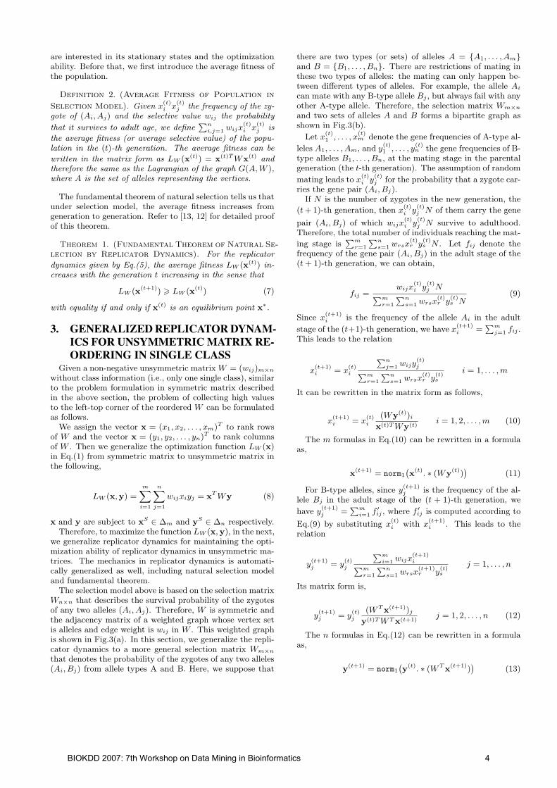
The selection model above is based on the selection matrixWn×n that describes the survival probability of the zygotesof any two alleles (Ai, Aj). Therefore, W is symmetric andthe adjacency matrix of a weighted graph whose vertex setis alleles and edge weight is wij in W . This weighted graphis shown in Fig.3(a). In this section, we generalize the repli-cator dynamics to a more general selection matrix Wm×n

that denotes the probability of the zygotes of any two alleles(Ai, Bj) from allele types A and B. Here, we suppose that

there are two types (or sets) of alleles A = {A1, . . . , Am}and B = {B1, . . . , Bn}. There are restrictions of mating inthese two types of alleles: the mating can only happen be-tween different types of alleles. For example, the allele Ai

can mate with any B-type allele Bj , but always fail with anyother A-type allele. Therefore, the selection matrix Wm×n

and two sets of alleles A and B forms a bipartite graph asshown in Fig.3(b).

Let x(t)1 , . . . , x

(t)m denote the gene frequencies of A-type al-

leles A1, . . . , Am, and y(t)1 , . . . , y

(t)n the gene frequencies of B-

type alleles B1, . . . , Bn, at the mating stage in the parentalgeneration (the t-th generation). The assumption of random

mating leads to x(t)i y

(t)j for the probability that a zygote car-

ries the gene pair (Ai, Bj).If N is the number of zygotes in the new generation, the

(t + 1)-th generation, then x(t)i y

(t)j N of them carry the gene

pair (Ai, Bj) of which wijx(t)i y

(t)j N survive to adulthood.

Therefore, the total number of individuals reaching the mat-

ing stage is∑m

r=1

∑ns=1 wrsx

(t)r y

(t)s N . Let fij denote the

frequency of the gene pair (Ai, Bj) in the adult stage of the(t + 1)-th generation, we can obtain,

fij =wijx

(t)i y

(t)j N

∑mr=1

∑ns=1 wrsx

(t)r y

(t)s N

(9)

Since x(t+1)i is the frequency of the allele Ai in the adult

stage of the (t+1)-th generation, we have x(t+1)i =

∑mj=1 fij .

This leads to the relation

x(t+1)i = x

(t)i

∑nj=1 wijy

(t)j∑m

r=1

∑ns=1 wrsx

(t)r y

(t)s

i = 1, . . . , m

It can be rewritten in the matrix form as follows,

x(t+1)i = x

(t)i

(Wy(t))i

x(t)T Wy(t)i = 1, 2, . . . , m (10)

The m formulas in Eq.(10) can be rewritten in a formulaas,

x(t+1) = norm1

(x(t). ∗ (Wy(t))

)(11)

For B-type alleles, since y(t+1)j is the frequency of the al-

lele Bj in the adult stage of the (t + 1)-th generation, we

have y(t+1)j =

∑mi=1 f ′ij , where f ′ij is computed according to

Eq.(9) by substituting x(t)i with x

(t+1)i . This leads to the

relation

y(t+1)j = y

(t)j

∑mi=1 wijx

(t+1)i∑m

r=1

∑ns=1 wrsx

(t+1)r y

(t)s

j = 1, . . . , n

Its matrix form is,

y(t+1)j = y

(t)j

(W T x(t+1))j

y(t)T W T x(t+1)j = 1, 2, . . . , n (12)

The n formulas in Eq.(12) can be rewritten in a formulaas,

y(t+1) = norm1

(y(t). ∗ (W T x(t+1))

)(13)


The state of the gene pool of the t-th generation is given

by the vector x(t) = (x(t)1 , . . . , x

(t)m )T of gene frequencies in

A-type alleles and the vector y(t) = (y(t)1 , . . . , y

(t)n )T of gene

frequencies in B-type alleles. x(t) and y(t) have non-negativecomponents summing up to one, and belong to the simplex∆m and ∆n respectively. Eq.(11) and Eq.(13) are the gen-eralized selection model for two types of alleles A and B. Itdescribes the action of selection between two types of alle-les from one generation to the next, and therefore the mapsending x(t) and y(t) to x(t+1) y(t+1) defines a discrete dy-namical system on the spaces ∆m and ∆n, called GeneralizedReplicator Dynamics (GRD).

Definition 3 (Generalized Replicator Dynamics).

Let Wm×n be a non-negative matrix. Given the vector x(t) =

(x(t)1 , . . . , x

(t)m )T ∈ Rm

+ and the vector y(t) = (y(t)1 , . . . , y

(t)n )T ∈

Rn+ being the status of the system in the t-th iteration, we de-

fine the discrete dynamical system as Eq.(11) and Eq.(13).

Correspondingly, we studied the the fixed points and opti-mization ability of generalized replicator dynamics. Next theaverage fitness of the population and the fundamental the-orem of natural selection in the generalized selection modelare given.

Definition 4. (Average Fitness of Population in

Generalized Selection Model). Given x(t)i y

(t)j the fre-

quency of the zygote of (Ai, Bj) and the selective value wij

the probability that it survives to adult age, we define∑mi=1

∑nj=1 wijx

(t)i y

(t)j is the average fitness (or average se-

lective value) of the population in the (t)-th generation. The

average fitness in the matrix form is LW (x(t),y(t)) = x(t)T Wy(t)

= y(t)T W T x(t) and therefore the same as the generalizedfunction of a bipartite graph G(A, B, W ), where A and Bare two sets of alleles representing the vertices.

Theorem 2. (Fundamental Theorem of Natural Se-lection by Extended Replicator Dynamics). For thegeneralized replicator dynamics given by Eq.(11) and Eq.(13),

the average fitness LW (x(t),y(t)) increases with the genera-tion t increasing in the sense that

LW (x(t+1),y(t+1)) > LW (x(t),y(t)) (14)

with equality if and only if x(t) and y(t) are two equilibriumpoints x∗ and y∗ respectively.

Proof. See http://www.utdallas.edu/∼ying.liu/BIOKDD2007.html

If let W be symmetric, x and y are associated with thesame set of vertices and thus equal to each other. HenceEq.(11) and Eq.(13) are reduced to Eq.(6) and thereforereplicator dynamics become a special instance of generalizedreplicator dynamics. In practice, the iteration of about 50 isenough for generalized replicator dynamics to get converged.Therefore, its computational complexity is O(k(2h+m+n)),where k is the number of iterations, h, m and n are thenumber of non-zeros, numbers of rows and columns in Wrespectively. If ignoring k, the final complexity is O(2h +m + n). Therefore, generalized replicator dynamics is veryefficient.

4. GENERALIZED ERD FOR UNSYMMET-RIC MATRIX REORDERING IN MUL-TIPLE CLASSES

In Section 2 and Section 3, we have shown how to discoverdistinct “mountain” within a single class by matrix reorder-ing. In this section, we shall focus on a more complicatedproblem of finding the“mountain”and“valley”which are col-lected parallel (i.e. with the same rows or genes/proteins)but on the left-top corner of each class submatrix 1. Thosegenes (or rows) which contribute to the parallel “mountain”and “valley” on the top of the reordered matrix, are deemedto be potential genes or proteins for biomarker. The moretop they are placed, the higher differential expressions theyhave. Those top-ranked genes in distinct parallel “moun-tain” and “valley” contribute much more differential expres-sions across negative and positive classes. Therefore, thesolution of parallel “mountain” and “valley” can not onlyrank differentially expressed genes, but also visually showthe expression values’ distribution within class (i.e., collect-ing low/high values to left-top corner of each class subma-trix) and between class (i.e., parallel collecting low and highvalues in negative and positive class respectively).

RD and GRD are designed to approach the problems ofcollecting the high values to the left-top corner of the matrixrearranged by the element orders of the solution x∗ and y∗.However, they only investigate the data which has no classlabels. In this section, a similar but more complicated task,parallel “valley and mountain” (up regulation) and paral-lel “mountain and valley” (down regulation) across multipleclasses, is considered. Because RD and GRD have beenproved that they are able to quickly approximate the opti-mization of the functions LW (x) and LW (x,y) respectively,such capability of reordering matrix can be introduced toour task of gene selection for biomarker discovery. In thefollowing, we will present how we customize and generalizeERD to our target in microarray data analysis.

Considering the general case of microarray data, supposethe data set consists of m genes and n samples with k classes,whose number of samples are n1, . . . , nk respectively andn1 + . . . + nk=n. Without losing the generality, we supposethe first k− classes are negative, the following k+ classes arepositive, and k−+k+ = k. Therefore, a general gene-samplematrix Wm×n = [ W−

i︸︷︷︸16i6k−

, W+i︸︷︷︸

16i6k+

] is shown with submatrix

blocks in Fig.4(a). Like fold change, the difference of valuesbetween negative and positive classes can show the up ordown tendency 2.

Because the target of analyzing differentially expressedgenes is to find up-regulated or down-regulated genes be-tween negative and positive sample classes, the basic reso-nance model should be changed, from collecting high valuesto the left-top corner of W ′, to:

1. Within-class data distribution: A series of low val-ues collections in each W−

i into the left-top corner,and simultaneously a series of high values collectionsin each W+

i into the left-top corner.

1Each sample class forms a submatrix where rows are thewhole set of genes and columns are the samples in this class.2The up tendency means that low values are in samples ofthe negative class, while high values are in samples of thepositive class. Vice versa for the down tendency.


2. Between-class data distribution: Controlling thedifferences of left-top corners between the negative classesW−

i and W+i .

Therefore, to meet these two goals, we extended gener-alized replicator dynamics, called EGRD, according to thistask as follows.

1. Transformation of W : before performing EGRD, weneed to transform the original gene-sample matrix Wto W ′. The structure of W is made of the submatrixblocks W−

i and W+i of negative classes and positive

classes as shown in Fig.4(a). In the case of findingup tendency and differentially expressed genes, sincewe need to collect the low values of W−

i into the left-top corner, we reverse the values of W−

i so that lowvalues become high and vice versa. In other words,we perform the transformation by W ′−

i = 1−W−i . In

this way, the result of collecting high values of W ′−i

and W ′+i into their own left-top corners naturally lead

to the result of collecting the low values of W−i into

the left-top corners and the high values of W+i into

the left-top corners. This is an essential step to meetthe first goal aforementioned. We can also use otherreverse functions in stead of the simple 1− x functionused in Fig.4(b). Similarly, we can transform W byW ′+

i = 1 −W+i in the case of finding down-regulated

and differentially expressed genes.

2. The k partitions of the allele set B: an implicit re-quirement in the first goal is that the relative orderof each class (submatrix W ′−

i or W ′+i ) should be kept

the same after performing EGRD and sorting W ′. Forexample, after running our algorithm, it is requiredthat all columns of the submatrix W ′−

2 appear afterall columns of W ′−

1 , although we can change the orderof columns or samples within W ′−

1 or W ′−2 . To sat-

isfy this requirement, we partition the original vectory of gene frequencies in B-type alleles into k parts cor-responding to k classes or submatrices. Specifically,y = (y1; . . . ;yk) 3, where each yi corresponds to asample class. In the process of EGRD, we separatelynormalize each yi and then sum them together withthe factor α to control the differentiation between thenegative and positive classes.

3. The factor α for controlling the differentiation betweenthe negative and positive classes: the gene frequencyvector of y is divided into k = k− + k+ parts, each ofwhich is normalized independently. Therefore, we cancontrol the differentiation between the negative andpositive classes, by magnifying the resonance strengths

x+(t+1)i = norm1(x

+(t). ∗ (W ′+i y

+(t)i )) of k+ positive

classes, or minifying the frequency subvectors x−(t+1)i =

norm1(x−(t). ∗ (W ′−

i y−(t)i )) of k− negative classes. In

formal,

x(t+1)

= norm1

(x−(t+1)1 + . . . + x

−(t+1)k−︸︷︷︸

k− negative classes

+ αx+(t+1)1 + . . . + αx

+(t+1)k+︸︷︷︸

k+ positive classes

)

(15)

3The concatenation of k = k− + k+ vectors is expressed inMATLAB format.

where α > 1 and α as a scaling factor is multiplied withthe normalized positive classes’ resonance strength vec-tors. With the increasing of α, the proportions of pos-itive classes in the gene frequency vector x will in-crease and thus result in the increasingly large differ-ences in the top-left corners between positive and neg-ative classes. In this way, the user can tune α to get asuitable differential contrast of two types of classes.

4. Smoothness of gene frequency vectors of B-type alle-les: In practice, we found that the partitioned genefrequency vectors of B-type alleles y+

i or y−i often con-verges to the extreme distribution of elements: few el-ements approach to 1 while the rest approximate to 0.Therefore, to smooth the element distribution of y+

i

and y−i , we introduced the sigmoid function 4 that iswidely used in neural networks. Therefore, we definethe new normalization function incorporating the sig-moid function as normsig1(y) = norm1(sig(norm1(y))).In this way, the gene frequency vectors are smoothed.We have made experiments to test the convergenceof the EGRD after using the normalization functionnormsig1. The empirical results show that it can quicklyconverge.

To summarize the above changes of the resonance model,we draw the architecture of the EGRD in Fig.5 and expressits process in the following formulas:

x−(t+1)i =norm1

(x(t). ∗ (W ′−

i y−(t)i )

), i = 1, . . . , k−

x+(t+1)i =norm1

(x(t). ∗ (W ′+

i y+(t)i )

), i = 1, . . . , k+

x(t+1) = norm1

( ∑k−i=1 x

−(t+1)i + α

∑k+

i=1 x+(t+1)i

)

y−(t+1)i =normsig1

(y−(t). ∗ ((W ′−

i )T x(t+1))), i = 1, . . . , k−

y+(k+1)i =normsig1

(y−(t). ∗ ((W ′+

i )T x(t+1))), i = 1, . . . , k+

(16)

where xi,x+i ,x−i ∈ Rm×1 and y−i ∈ Rn−i ×1, y+

i ∈ Rn+i ×1.

Comparing Eq.(11) and Eq.(13) in GRD with Eq.(16), wepartitioned the matrix W ′ to k submatrix blocks and di-vided the gene frequency vector of B-type alleles y into ksubvectors. Therefore, two equations in the extended repli-cator dynamics are expanded to the (2k + 1) equations inEGRD.

Algorithm of EGRD will appear here. We also formallysummarize it as Algorithm 1 EGRD for the data reliabilityassessment.

In practice, GERD can quickly converge. Considering thatEGRD is a extended generalized replicator dynamics by par-titioning the matrix into k submatrices, its computationalcomplexity is the same as the extended replicator dynamicson the whole matrix, i.e., O(2h + m + n).

5. EXPERIMENTAL RESULTSIn this section, we conducted the experiments on the Leukemia

data set and compared our method with five popular filterfeature selection methods, T-statistics (T) [14], InformationGain (IG) [5], ReliefF [15], Correlation-based Feature Selec-tion (CFS) [11] and Redundancy Based Filter (RBF) [19].

4The sigmoid function is defined on the scalar num-ber x as, sig(x) = 1

1+exp(−x). Therefore, for a vec-

tor x, the corresponding sigmoid function is sig(x) =(sig(x1), . . . , sig(xn)

)T


… ...

......

Negative Classes Positive Classes

n = n1 + … + nk

n1 nk

-1W -

k-W W

+1

W+k+

... ... ... ...

W =

up regulation down regulation

W ′−i = 1−W−

i W−i

W ′+i = W+

i 1−W+i

W ′ = [1−W−i︸︷︷︸

16i6k−

, W+i︸︷︷︸

16i6k+

] [ W−i︸︷︷︸

16i6k−

, 1−W+i︸︷︷︸

16i6k+

]

(a) original matrix W = [ W−i︸︷︷︸

16i6k−

, W+i︸︷︷︸

16i6k+

] (b) transformed matrix W ′ = [ W ′−i︸︷︷︸

16i6k−

, W ′+i︸︷︷︸

16i6k+

]

Figure 4: Transformation of the matrix W : the transformed matrix W ′ has the same structure of submatrixblocks as shown in (a), but with different submatrix W ′−

i and W ′+i as listed in (b).

A1

B11

B21A2

Bk1Am

...

......

......

wij

Class 1

Class 2

Class k

Figure 5: Alleles Ai and Bl with k classes as verticesand their mating survival probabilities wij as edgeweights in generalized extended replicator dynam-ics.

Among them, the first three methods are based on the method-ology of ranking relevant genes; while the last two methods,i.e., CFS and RBF, do not rank genes, but aim to select aminimum gene subset with optimum feature relevance andreduced redundancy. Therefore, in the experiments, CFSand RBF only report the number of minimum gene sub-set discovered. We firstly used the EGRD 5, T and IG torank the genes and compared them over different featuresizes, k=2,4,10,20,50,100,200. Each resulting feature subsetwas used to train an SVM classifier 6 with the linear ker-nel function. Because of the small number of samples, theLeave-One-Out Cross Validation (LOOCV), a popular per-formance validation procedure adopted by many researchers,was performed to assess the classification performance.

5.1 Leukemia DataWe used the Leukemia gene expression data [2], where

besides the classes “ALL” (Acute Lymphoblastic Leukemia)and “AML” (Acute Myelogenous Leukemia), a new class

5Because EGRD can rank genes/proteins in terms of upand down regulation respectively, in this experiment ofcomparing k top-ranking genes/proteins, we selected 0.5ktop-ranking genes/proteins in up regulation and 0.5k top-ranking genes/proteins in down regulation to form k top-ranking genes given by EGRD.6The SVMlight was used.

Algorithm 1 EGRD

Input: (1) Wm×n, genomic or proteomic matrix from mgene set G and n samples set S;

(2) (n1, . . . , nk)T , sizes of the k sample classeswith the submatrix structure as in Fig.4(a).

(3) (k−, k+)T , numbers of negative and positiveclasses.

(4) tendency option, down or up;(5) α, differentiation factor.

Output: (1) (g1, . . . , gm), ranking sequence of m genes;(2) (s1, . . . , sn), ranking sequence of n samples.

1: preprocess W so that the values of W in [0,1].2: transform W to W ′ according to formulas in Fig. 4(b)

with the knowledge of the matrix structure given by(n1, . . . , nk)T , and (k−, k+)T and tendency option.

3: iteratively run formulas in Eq.(16) to obtain the con-verged x∗ and y∗i (i=1, 2, . . . , k).

4: sort x∗ in decreasing order to get the ranking sequence(g1, . . . , gm), and sort each of y∗1 , . . . ,y∗k in decreasingorder to get the sorted sample sequence {comment: Be-cause the positions of all sample classes in W ′ keep notchanging as shown in Fig.4(a), each sorting of y∗i canonly change the order of samples within the i-th sampleclass W ′

i .}.

of “MLL” (Mixed-Lineage or Myelogenous/LymphoblasticLeukemia) samples was identified. It contains 12,582 genesand 72 samples with these 3 sample classes. Therefore, weperformed three experiments to test our method by usingone class versus the rest of classes as positive versus negative:(1) ALL versus MLL&AML, (2) MLL versus ALL&AMLand (3) AML versus ALL&MLL. In each experiment, thegene expression matrix partition for our method is W =[W−

1 , W+1 , W+

2 ] with one negative and two positive classes.In all three experiments, α was set to 10 for EGRD. Theresults are shown in Table 1, 2 and 3. As shown in the threetables, our method EGRD outperforms the other methodsin,

• High Accuracy: in all three experiments, EGRD main-tains very high accuracies in different k. In the experi-ment “MLL versus ALL&AML”, where the class MLL


is hard to distinguish, EGRD can still obtain high ac-curacy even when k is very small.

• Compact biomarker: observing the accuracies of threemethods from the small k to the large, EGRD is ableto quickly obtain high accuracies even when k is small,while the methods T and IG require larger k to arriveat the same accuracy (the numbers in bold in threetables show the minimum k each method requires toget the highest accuracy). This means that EGRDoutperforms the other methods in terms of discoveringthe compact or minimal biomarker. For example, inTable 1, the top 2 ranking genes discovered by EGRDcan achieve 95.8% classification accuracy, while the ac-curacies of the other two methods’ top 2 ranking genesare less than 80%. Similar cases also appear in Table 2and 3.

• Stability: not only can the small number of selectedgenes achieve higher accuracies than the other meth-ods, but also as k increases (more biomarkers were se-lected), high classification accuracies are maintained.This is a stable property with k increasing, and may beinteresting to the biologists when they try to analyzemore relevant genes contributing to the diseases.

Table 1: LOOCV accuracy rate (%) of ALL versusMLL&AML.

k= 2 4 10 20 50 100 200

T 79.2 86.1 91.7 93.1 98.6 98.6 98.6

IG 76.4 80.6 95.8 98.6 98.6 98.6 98.6

RliefF 63.9 86.1 95.8 95.8 98.6 98.6 100

EGRD 95.8 100 100 100 100 100 100

CFS: find 55 genes with 100%

RBF: find 2 genes with 91.7%

Table 2: LOOCV accuracy rate (%) of MLL versusALL&AML.

k= 2 4 10 20 50 100 200

T 69.4 65.2 81.9 80.6 84.7 86.1 93.1

IG 72.2 88.9 88.9 88.9 98.6 98.6 97.2

RliefF 72.2 88.9 95.8 94.4 94.4 94.4 97.2

EGRD 84.7 91.7 97.2 98.6 100 98.6 98.6



Table 3: LOOCV accuracy rate (%) of AML versusALL&MLL.

k= 2 4 10 20 50 100 200

T 66.7 77.8 97.2 98.6 100 98.6 97.2

IG 79.2 76.4 87.5 93.1 97.2 97.2 97.2

RliefF 86.1 84.7 95.8 94.4 97.2 97.2 97.2

EGRD 88.9 94.4 97.2 97.2 97.2 97.2 98.6



An important factor, which enables EGRD to performwell, is that the matrix reordering has the global search-ing ability to take into account the value distribution ofthe whole matrix with multiple classes. This is differentfrom the way of individually considering genes, samples, orgene-to-gene. Our ultimate goal is to obtain the minimalbiomarker while keeping a relatively high classification accu-racy. In the experiment of “ALL versus MLL&AML”, com-pact biomarker is already discovered by EGRD because, forthe 4 genes selected, EGRD can achieve 100% accuracy. Inthe third experiment as listed in Table 3, we found 4 geneswhich achieve the accuracy 94.4% with EGRD. Similarly, inthe third experiment, although CFS can obtain 100% accu-racy, the size of the biomarker it discovers is too big (147genes). On the contrary, our method achieves the accuracy95.8% while the size of the biomarker is very small (only 2genes).

To test if the biomarker found by our methods is biologi-cally meaningful or not, for instance, we checked two genesfound by EGRD in Table 1 with Entrez Gene in NCBI Web-site (http://www.ncbi.nlm.nih.gov/entrez). These twogenes are MME, which is underexpressed, and LGALS1,which is overexpressed. By investigating the result of Arm-strong et al. [2], these two genes were also ranked as thefirst genes in the underexpressed and overexpressed genes re-spectively. MME is a common acute lymphocytic leukemiaantigen which is an important cell surface marker in the di-agnosis of human acute lymphocytic leukemia (ALL); whileLGALS1 was also reported to be highly correlated withALL [17].

5.2 ConclusionIn this work, we have introduced a novel perspective of

matrix reordering for ranking both genes and samples inmultiple-class microarray data. It comprehensively consid-ers the global between-class data distribution and local within-class data distribution, and therefore improves the accuracyof the biomarker discovery. Meanwhile, it identifies an over-all tendency of the whole matrix for analyzing the data.Experiments on microarray data have demonstrated its effi-ciency and effectiveness of both visualization and biomarkerdiscovery.

6. REFERENCES[1] P. Amestoy, T. Davis, and I. Duff. An approximate

minimum degree ordering algorithm. SIAM Journalon Matrix Analysis and Applications, 17(4):886–905,1996.

[2] S. Armstrong and et. al. MLL translocations specify adistinct gene expression profile that distinguishes aunique leukemia. Nature Genetics, 30(1):41–47, 2002.

[3] L. E. Baum and J. A. Eagon. An inequality withapplications to statistical estimation for probabilisticfunctions of markov processes and to a model forecology. Bull. Amer. Math. Soc., 73:360lC363, 1967.

[4] M. Berry, B. Hendrickson, and P. Raghavan. Sparsematrix reordering schemes for browsing hypertext. InProc. of the AMS-SIAM Summer Seminar onMathematics of Numerical Analysis: Real NumberAlgorithms, Park City, UT, 1995.

[5] T. Cover and J. Thomas. Elements of InformationTheory. Wiley, New York, 2nd edition, 2006.


[6] J. Crow and M. Kimura. An Introduction toPopulation Genetics Theory. Harper & Row, NewYork, 1970.

[7] E. Cuthill and J. McKee. Reducing the bandwidth ofsparse symmetric matrices. Proc. of the 24th NationalConference of the ACM, 1969.

[8] C. Ding and H. Peng. Minimum redundancy featureselection from microarray gene expression data.Journal of Bioinformatics and Computational Biology,3(2):185–205, 2005.

[9] D. L. Donoho. High-dimensional data analysis: Thecurses and blessings of dimensionality. MathChallenges of the 21st Century, August 2000.

[10] W. Gansterer and T. Korimort. Matrix reordering byhypertree decomposition. Technical Report AURORATR2003-19, University of Vienna, 2003.

[11] M. Hall. Correlation-based feature selection fordiscrete and numeric class machine learning. In Proc.of ICML, pages 359–366, 2000.

[12] J. Hofbauer and K. Sigmund. The Theory of Evolutionand Dynamical Systems. Cambridge University Press,1988.

[13] J. Hofbauer and K. Sigmund. Evolutionary Games andPopulation Dynamics. Cambridge University Press,1998.

[14] R. Johnson and D. Wichern. Applied MultivariateStatistical Analysis. Prentice Hall, New Jersey, 5thedition, 2002.

[15] K. Kira and L. Rendell. A practical approach tofeature selection. In Proc. of ICML, 1992.

[16] M. Pelillo. The dynamics of nonlinear relaxationlabeling processes. J. Math. Imaging Vision,7(4):309lC323, 1997.

[17] T. Rozovskaia and et. al. Expression profiles of acutelymphoblastic and myeloblastic leukemias with all-1rearrangements. Proc. of National Academy ofSciences USA, 100(13):7853–7858, 2003.

[18] I. Tabus and J. Astola. Genomic Signal Processingand Statistics, chapter Gene Feature Selection.Hindawi Publishing Corporation, 2005.

[19] L. Yu and H. Liu. Redundancy based feature selectionfor microarray data. In Proc. of SIGKDD, pages737–742, Seattle, 2004.


Investigating the use of Extrinsic Similarity Measures forMicroarray Analysis ∗

D. Ucar, F. Altiparmak, H. Ferhatosmanoglu and S. Parthasarathy†

Department of Computer Science and EngineeringThe Ohio State University

Columbus, OhioContact : [email protected]

ABSTRACTGenes behaving similarly over changing conditions are be-lieved to be part of the same functional module. Identify-ing functional modules of genes plays an important role inunderstanding gene regulatory behavior as well as in facili-tating function prediction of unknown genes. Subsequently,determining ‘similar’ gene pairs or groups based on theirgene expression profiles is an important task towards ex-tracting modules from microarray datasets. A prevailingtechnique is to use a linear similarity measure like Pearson’scorrelation coefficient or Euclidean distance, to find simi-lar gene pairs. However, the noise inherent in microarraydatasets reduces the sensitivity of these measures and pro-duces many spurious pairs with no real biological relevance.In this paper, we explore an extrinsic way of calculatinggene similarity based on their relations with other genes.We show that ‘similar’ pairs identified by extrinsic measuresoverlap better with known biological annotations availablein the Gene Ontology database. Our results also indicatethat extrinsic measures are useful to enhance the quality ofgene networks constructed from similar gene pairs by reduc-ing spurious edges and introducing missing edges betweennetwork nodes.

Categories and Subject DescriptorsH.2.8 [Database Applications]: Data Mining

KeywordsBioinformatics, Microarray analysis, Extrinsic similarity

1. INTRODUCTION AND RELATED WORK∗This work is supported in part by DOE Early Career Prin-cipal Investigator Award No. DE-FG02-04ER25611 andNSF CAREER Grant IIS-0347662.†To whom correspondence should be addressed.

Permission to make digital or hard copies of all or part of this work forpersonal or classroom use is granted without fee provided that copies arenot made or distributed for profit or commercial advantage and that copiesbear this notice and the full citation on the first page. To copy otherwise, torepublish, to post on servers or to redistribute to lists, requires prior specificpermission and/or a fee.BIOKDD’07 August 12, 2007, San Jose, California,USA.Copyright 2007 ACM 978-1-59593-839-8/07/0008 ...$5.00.

Due to advances in technology (e.g., oligonucleotide mi-croarray chips), scientists are now able to accumulate awealth of information on the expression of genes during thelife cycle of an organism. Such datasets provide vital in-formation that can be used to gain insight into diverse bi-ological questions. To analyze and mine these datasets forpotential useful information, various techniques and ideashave been proposed. Of particular interest to many scien-tists is the problem of identifying gene groups that havesimilar expression patterns over various samples, known asco-expressed genes. Genes with similar cellular functionshave been theorized to behave similarly over different con-ditions [10]. Thus, obtaining groups of similar genes is fun-damental to understanding the molecular and biochemicalprocesses that sustain the physiological state of the cell [23].

There has been a growing interest in representing co-expressedgenes as an association network to explore the system-levelfunctionality of genes [25, 6]. Here, nodes represent genesand two nodes are linked if the corresponding genes aresignificantly co-expressed (correlated) across the samples.Earlier approaches have used expression levels of two genesover all samples to surmise their correlation. However, thissimilarity notion does not necessarily imply that genes arefunctionally related. Given the noise inherent in microarraydatasets, it is our hypothesis that intrinsic similarity mea-sures are not adequate to distinguish accidentally regulatedgenes from those that are biologically motivated. We ar-gue that since any given gene is likely to fluctuate in itsmeasured expression level due to many possible sources oferror, a similarity based on two genes’ measurements is moreerror-prone than using relative positions of many genes asa reference to deduce the same information. In addition,gene products act as complexes to accomplish certain cellu-lar level tasks [22], which is potentially suitable to infer twogene’s similarity via their relations with other genes. Thus,we propose and investigate the use of extrinsic similaritymeasures to induce gene similarity.

The use of extrinsic measures and their advantages havebeen previously studied for various data mining problems [8,9]. Das et al [8], proposed using extrinsic measures on mar-ket basket data in order to derive similarity between twoproducts from the buying patterns of customers. Palmer etal [18], defined an extrinsic similarity measure (REP) withan analogy to electric circuits. Both groups concluded thatextrinsic measures can give additional insight into the data.Recently, Ravasz et al [19], proposed the Topological Over-lap Measure (TOM), which is one of the few to use extrinsic


properties along with the intrinsic ones. Their measure in-fers similarity of two nodes in a biochemical network in termsof their pairwise similarity as well as the number of commonneighbors they share.

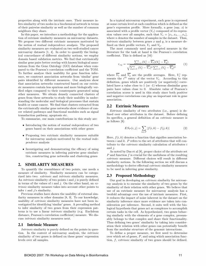
In this paper, we introduce a methodology for the applica-tion of extrinsic similarity measures on microarray datasets.We propose two different extrinsic measures motivated bythe notion of mutual independence analysis. The proposedsimilarity measures are evaluated on two well-studied cancermicroarray datasets [1, 4]. In order to quantify the biolog-ical concordance of different similarity notions, we employdomain based validation metrics. We find that extrinsicallysimilar gene pairs better overlap with known biological anno-tations from the Gene Ontology (GO) database when com-pared to the Pearson’s correlation coefficient and the TOM.To further analyze their usability for gene function infer-ence, we construct association networks from ‘similar’ genepairs identified by different measures. Our analyzes showthat association networks constructed based on our extrin-sic measures contain less spurious and more biologically ver-ified edges compared to their counterparts generated usingother measures. We obtain densely connected clusters ofgenes from these networks to study their usability in under-standing the molecular and biological processes that sustainhealth or cause cancer. We find that clusters extracted fromthe extrinsically similar gene networks show evidence of can-cer related pathways and functional modules such as signaltransduction pathway, apoptosis etc.

To summarize, our main contributions in this study are:

• Introducing the notion of mutual independence of twogenes based on their associations with other genes

• Proposing two extrinsic similarity measures suitablefor microarray analysis motivated by the mutual inde-pendence analysis

• Investigating and demonstrating the efficacy of usingextrinsic measures in inferring pairwise gene similari-ties, constructing gene networks and clustering genes

2. SIMILARITY MEASURESTo quantify the resemblance of two points, one needs a

measure of similarity. Similarity measures can be catego-rized into two: extrinsic and intrinsic similarity measures.An intrinsic similarity of two points i and j is purely definedin terms of the values of i and j. On the other hand, an ex-trinsic similarity measure takes into account other points toinfer i and j’s similarity.

Previous studies have shown the usability of external sim-ilarity measures in other domains [8, 9]. To our knowledge,usability of extrinsic similarity measures have not been in-vestigated for identifying ‘similar’ genes. A prevailing methodto infer similarity of two genes from their expression pat-terns is to use a linear intrinsic similarity (e.g. Euclideandistance, Pearson’s correlation coefficient) measure. We dis-cuss intrinsic similarity measures next.

2.1 Intrinsic MeasureIntrinsic similarity is purely defined on the points in ques-

tion. In the context of microarray analysis, the intrinsicsimilarity of two genes is defined on these genes’ expressionlevels over all samples.

In a typical microarray experiment, each gene is expressedat some certain level at each condition which is defined as thegene’s expression profile. More formally, a gene (say, x) isassociated with a profile vector (Vx) composed of its expres-sion values over all samples, such that Vx = [x1, x2, ..., xn],where n denotes the number of samples in the dataset. Thus,intrinsic similarity between genes x and y, is a measure de-fined on their profile vectors, Vx and Vy.

The most commonly used and accepted measure in theliterature for the task at hand is the Pearson’s correlationcoefficient. This is defined as [16]:

rxy =

Pn

i=1 (V ix − Vx)(V i

y − Vy)q

Pn

i=1 (V ix − Vx)2

Pn

i=1 (V iy − Vy)2

(1)

where Vx and Vy are the profile averages. Here, V ix rep-

resents the ith entry of the vector Vx. According to thisdefinition, genes which are positively (or negatively) corre-lated have a value close to 1 (or -1) whereas dissimilar genepairs have values close to 0. Absolute value of Pearson’scorrelation scores is used in this study since both positiveand negative correlations can play an important role in geneassociation.

2.2 Extrinsic MeasuresExtrinsic similarity of two attributes (i.e., genes) is de-

fined over other attributes in the dataset. Before definingits specifics, a general definition of an extrinsic measure isas follows [8]:

ESP (i, j) =X

k∈P

|f(i, k) − f(j, k)| (2)

Here, f(i, k) denotes a function that signifies association be-tween i and k. P refers to the set of attributes that will con-tribute to the extrinsic similarity calculation of attributes i

and j.As noted by Das et al [8], proper choice of the attribute set

P and function f is crucial for the usefulness of the resultingextrinsic measure. Different choices will result in differentsimilarity notions. In the following section we will discuss amethodology to derive effectual extrinsic similarity measuresto be used in inferring gene similarity.

2.3 Proposed MethodologyOur goal in developing an extrinsic similarity for microar-

ray analysis is to surmise the similarity of two genes by thesimilarity of their relation with other genes. We believe thatuse of an extrinsic measure for microarray analysis has atwofold advantage over the use of intrinsic measures. First,it reduces the impact of noise inherent in the dataset on thesimilarity inference since more evidence are taken into con-sideration per inference. Second, it suits well with the bio-logical hypothesis that genes act as complexes to accomplishcertain tasks in the cell. As hypothesized, two genes behav-ing similarly with the elements of a gene complex, presum-ably belongs to that complex and share their functionality.Thus defining two genes’ similarity by taking into consider-ation their relation with other genes can potentially benefitfrom the modular structure of the genomic interactions.

To define a proper measure, we first need to determineover which set of genes, P , and using which association func-tion, f , extrinsic similarity of two genes should be defined.


Here, we investigate the use of close proximity of genes ac-cording to intrinsic notions when choosing a proper set P . Inaddition, two functions based on mutual independence anal-ysis from the Information Theory are evaluated. We com-pare the proposed similarity measures with the currentlyavailable techniques described in Section 3, as well as themost popular intrinsic measure (i.e., Pearson’s correlationcoefficient).

2.3.1 Choice of Attribute Set (P )To derive an efficient extrinsic measure for microarray

analysis, we first need to identify a gene set, P , that willbe used to infer the extrinsic similarity of two genes. Forthis purpose, we use the group of genes that are similar toboth of the genes under question. Thus, initially for eachgene we identify a set of genes that are intrinsically similarto that gene (i.e., the gene’s close neighbors). We refer thisas a gene’s neighborhood list (Ni) and define it as follows:

Ni = {j|j ∈ G, |rij | > κ} (3)

Here, G denotes the set of all genes in our dataset and |rij |refers to the absolute value of the Pearson’s correlation coef-ficient of genes i and j. Effect of the threshold parameter κ,on the extrinsic measures and guidance of the size of neigh-borhood lists to set this parameter is discussed in Section 61.Next, the attribute set P that will be used to infer two genes’similarity is designated as the intersection of their neighbor-hood lists (i.e., P = Ni ∩ Nj ). Using common neighborsof two genes as the set of attributes (P ) has two impor-tant implications. First, it significantly reduces the requirednumber of calculations. Thus, instead of using the wholegene set (G), a smaller size set is taken into consideration.Secondly, it filters out irrelevant information which improvesthe success of the extrinsic measure. By using the intrinsicsimilarity to determine elements in set P , we take advantageof both extrinsic and intrinsic properties. Our hypothesisis that this helps to reduce the noisy inference that can beintroduced into the similarity inference by using these mea-sures separately. It is noteworthy that an extrinsic measurecan be easily expandable to other groups of related genes.For instance, one can prefer using an attribute set contain-ing genes mapped to close chromosomal locations with twogenes whose similarity is under investigation.

2.3.2 Choice of Association Function (f)After establishing the notion of an extrinsic similarity, and

defining the set P , the next step is to determine which asso-ciation function (f) to use for our calculations. Das et al [8],proposed using the confidence of association rules in an ap-plication on market basket dataset. Their approach and itsapplicability on gene expression datasets will be discussedin details in Section 3. We propose using two appropriatefunctions that are motivated by the mutual independenceanalysis. We leverage mutual independence of two genes byanalyzing their frequency of occurrence and co-occurrencein the neighborhood lists.

Before defining mutual dependency of two genes, first, weexplore three possible type of relations between any twogenes motivated by Das et al [8]. Accordingly, two genescan either be, complementary, independent or correlated. Iftwo genes are complementary, then they do not to co-occur

1Our analysis indicated that relatively loose values producemore useful extrinsic measures.

in the neighborhood lists. If they are independent, neighborsof gene i are neighbors of gene j with the same probabilityas the genes that are not neighbors of gene i. And if theyare correlated, neighbors of gene i are also neighbors of genej. These concepts are formally defined using neighborhoodlists as follows:

Definition 1: Frequency of occurrence for a gene i, P (i),is defined as the frequency of encountering that gene in allneighborhood lists. Since Pearson’s correlation coefficient isa symmetric measure a gene has as many neighbors as thenumber of times it occurs in all neighborhood lists. Thus,frequency of a gene’s occurrence can be simplified to thefollowing:

P (i) =|Ni|

|G|(4)

where ‘|u|’ denotes the number of elements (cardinality) inits argument. Note that frequency of occurrence is an in-dication of the discriminatory nature of a gene’s expressionprofile. Genes with indistinct expression profiles such as thehousekeeping genes will have higher values of frequency ofoccurrence.

Definition 2: Frequency of co-occurrence for genes i andj, P (i, j), is defined as the frequency of encountering thesetwo genes together in the neighborhood lists. More formally,based on the symmetric Pearson’s measure, P (i, j) can bedefined as follows:

P (i, j) =|{a|a ∈ G, i ∈ Na, j ∈ Na}|

|G|(5)

By itself high frequency of co-occurrence does not implythat two genes are correlated. In order to conclude that twogenes are not randomly co-occurring (independent) but thereis a biological trigger behind their co-occurrence (correlated),we need to test if one gene’s frequency of occurrence is helpfulin predicting that of the other gene which is a notion knownas mutual independence. Note that, in this context, inde-pendence of two genes implies that occurrence of a gene in aneighborhood list makes it neither more nor less probable forthe other gene to occur in that list. Thus, mutual indepen-dence of two genes only holds when P (i, j) = P (i)P (j). Wepropose using two different independence tests to leveragemutual dependency of two genes.

Specific Mutual Information Measure:

The Specific Mutual Information (smi) is a measure of as-sociation commonly used in the Information Theory to infermutual dependency. Smi of two variables, X and Y , giventheir joint distribution, P (X, Y ), and individual distribu-tions, P (X) and P (Y ), is defined as follows:

I(X,Y ) =O

E=

P (X, Y )

P (X)P (Y )(6)

where P (X,Y ) is the observed value (O) for joint probabilityof events X and Y , whereas P (X)P (Y ) is its expected value(E).

This test can be used to deduce the type of relation be-tween two genes. If their smi value is 1, it can be concludedthat these two genes are independent. On the other hand,a value greater than 1 implies being correlated and a valuesmaller than 1 implies being complementary.


If two genes have similar relations with their commonneighbors, it is reasonable to conclude that they are simi-lar. Based on this analysis and the notion of specific mutualinformation, we propose the following extrinsic measure toquantify dissimilarity of two genes (i and j).

smiP (i, j) =

P

k∈P |P (i,k)

P (i)P (k)−

P (j,k)P (j)P (k)

|

|P |(7)

This definition ensures that two genes having similar rela-tions (i.e., complementary, correlated or independent) withtheir common neighbors are closely related to each other(smi value close to 0). Whereas two genes that have dif-ferent relations with their common neighbors are dissimilarand associated with higher values of smi. Note that, thesmi measure is normalized by dividing by the size of theattribute set P .

Chi-Square Based Measure:

Pearson’s chi-square test is another method to assess mutualdependency of two events. Formally, it is defined as follows:

chi(X, Y ) =(O − E)2

E=

(P (X,Y ) − P (X)P (Y ))2

P (X)P (Y )(8)

This test tells us how far the observed value deviates fromthe expected value under the assumption of independence.

According to this definition, two genes will have zero chi

value if they are independent. They will have higher chi

values otherwise. We employ a signed version of this test tosurmise the type of relation between two genes. Given this,external dissimilarity of two genes based on the chi-squareanalysis, chiP (i, j), is defined as follows:

P

k∈P |sik(P (i,k)−P (i)P (k))2

P (i)P (k)−

sjk(P (j,k)−P (j)P (k))2

P (j)P (k)|

|P |(9)

where sab denotes the sign of the term P (a, b) − P (a)P (b).Note that signs are included into the measure to differen-tiate a correlated pair from a complementary one. Similarto the smi measure, two genes that have similar relationswith their common neighbors will have smaller chi valueswhereas two genes that have dissimilar relations with theircommon neighbors will have higher values2. Chi measure isalso normalized by dividing by the size of the attribute set.

3. PREVIOUS WORK

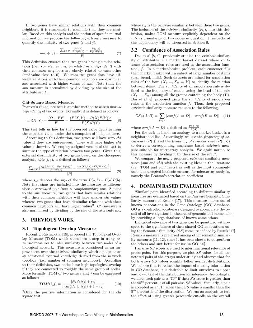
3.1 Topological Overlap MeasureRecently, Ravasz et al [19], proposed the Topological Over-

lap Measure (TOM) which takes into a step in using ex-trinsic measures to infer similarity between two nodes of abiological network. This measure is considered as an im-provement over the intrinsic similarity which amalgamatesan additional external knowledge derived from the networktopology (i.e., number of common neighbors). Accordingto their definition, two nodes have high topological overlapif they are connected to roughly the same group of nodes.More formally, TOM of two genes i and j can be expressedas follows:

TOM(i, j) =|Ni ∩ Nj | + rij

min{|Ni|, |Nj |} + 1 − rij

(10)

2Only the positive information is considered for the chisquare test.

where rij is the pairwise similarity between these two genes.The inclusion of the intrinsic similarity (rij), into this def-inition, makes TOM measure explicitly dependent on theintrinsic similarity of two nodes in question. Drawbacks ofthis dependency will be discussed in Section 6.

3.2 Confidence of Association RulesDas et al [8, 9], previously studied the extrinsic similar-

ity of attributes in a market basket dataset where confi-dence of association rules are used as the association func-tion, f . In a market-basket problem, each customer fillstheir market basket with a subset of large number of items(e.g., bread, milk). Such datasets are mined for associationrules of the form (X1, ..., Xn ⇒ Y ) to identify the relationbetween items. The confidence of an association rule is de-fined as the frequency of encountering the head of the rule(X1, ..., Xn) among all the groups containing the body (Y ).Das et al [8], proposed using the confidence of associationrules as the association function f . Thus, their proposedextrinsic similarity measure reduces to the following.

ESP (A,B) =X

D∈P

|conf(A ⇒ D) − conf(B ⇒ D)| (11)

where conf(A ⇒ D) is defined as P (A,D)P (A)

.

For the task at hand, an analogy to a market basket is aneighborhood list. Accordingly, we use the frequency of oc-currence (P (i)) and the frequency of co-occurrence (P (i, j))to derive a corresponding confidence based extrinsic mea-sure suitable for microarray analysis. We again normalizethis measure by dividing it by the size of the set P .

We compare the newly proposed extrinsic similarity mea-sures (smi and chi) with the existing ideas in the literature(i.e., TOM and confidence) as well as the most commonlyused and accepted intrinsic measure for microarray analysis,namely the Pearson’s correlation coefficient.

4. DOMAIN BASED EVALUATION‘Similar’ pairs identified according to different similarity

measures are evaluated based on the Pairwise Semantic Sim-ilarity measure of Resnik [17]. This measure makes use ofknown annotations in the Gene Ontology (GO) database.GO is a controlled vocabulary designed to accumulate the re-sult of all investigations in the area of genomic and biomedicineby providing a large database of known associations.

Biological relevance of two genes can be quantified with re-spect to the significance of their shared GO annotations us-ing the Semantic Similarity (SS) measure defined by Resnik [17].Resnik’s measure is preferred among other semantic similar-ity measures [11, 12], since it has been shown to outperformthe others and suit better for use in GO [20].

Pairwise SS scores are used to infer functional relevance ofprobe pairs. For this purpose, we plot SS values for all an-notated pairs of the arrays under study and observe that forboth arrays SS values roughly follow normal distributions.We believe that to reduce the impact of missing informationin GO database, it is desirable to limit ourselves to upperand lower tail of the distribution for inference. Accordingly,we label each pair as a ‘TP’ if their SS score is greater thanthe 95th percentile of all pairwise SS values. Similarly, a pairis accepted as a ‘FP’ when their SS value is smaller than the5th percentile of the distribution. We run an analysis to testthe effect of using greater percentile cut-offs on the overall


results which is presented in the Experiments section. Wewant to note that, not every gene pair will be classified as a‘TP’ or a ‘FP’ using this labeling methodology. A pair thatis composed of at least one unannotated gene is not labeledsince there is not enough information to conclude about thebiological concordance of these two genes. In addition, agene pair with an SS score between the percentile cut-offs isnot labeled since considering it as a ‘TP’ or a ‘FP’ pair is amatter of specifying the granularity of biological similarity.

Pairs extracted by using different similarity notions are ac-cumulated into association networks. We define the Cluster-wise Positive Predictive Value measure (CPPV ) to evaluatethe biological quality of the dense regions extracted fromthese clusters. CPPV of a cluster, (say, Ci), is defined as

CPPVi = |TPi||TPi|+|FPi|

. Here, TPi and FPi denote the set

of ‘TP’ and ’FP’ pairs in that cluster. Our calculations arebased on every possible gene pair in a cluster. Higher valuesof CPPV imply that the cluster is enriched in ‘TP’ pairs.On the contrary, lower values indicate that the cluster iscomposed of biologically dissimilar genes.

5. DATASETS AND PRE-PROCESSINGFor this study, we employ two well-studied cancer datasets.

First dataset is composed of gene expression values of 62colon tissue samples where the Affymetrix Hum6000 arraywith 6819 probes is used [1]. 42 of these are collected fromcolon adenocarcinoma patients and 20 of them are collectedfrom normal colon tissue of the patients. Among all probes,2000 were selected from 6817 by Alon et al according to thehighest minimum intensity [1]. Second dataset is composedof 86 lung adenocarcinoma and 10 normal samples which isanalyzed by the Affymetrix HuGene FL array [4]. Beer etal [4] trimmed the dataset of genes expressed at extremelylow levels resulting in 4966 probes for investigation.

Initially, we consider 2000 and 4966 probes for colon andlung adenocarcinoma datasets respectively. We perform thresh-olding, log transformation and normalization (quantile nor-malization) on these two datasets as suggested by our anal-ysis. In addition to these, we further standardize datasetsusing a robust standardization method, median absolutedeviation (MAD). Genes with zero MAD values implyingthat they are co-expressed at very similar levels across all ofthe samples are excluded from further analysis. After pre-processing 1578 genes for colon cancer and 4228 genes forlung cancer datasets are examined.

6. EXPERIMENTSWe discuss the usability of external similarity measures as

a way of identifying similar genes throughout this section.First, we give results for biological relevance of gene pairsthat are identified as ‘similar’ with different measures. Then,co-expression networks generated from these ‘similar’ pairsare analyzed for biological soundness. Finally, genes in eachof these networks are clustered to study the effect of extrinsicsimilarity on the quality of gene clustering.

6.1 Setting the κ parameterBefore comparing newly proposed measures with the ex-

isting ones, we first investigate the effect of κ parameter onthe neighborhood lists. To choose a suitable κ threshold,there are two things that we should take into consideration.First, we want a gene’s neighborhood list to be composed

only of genes that are within close proximity of that gene.Second, it is not desirable to have a set that is only composedof a few genes since this would limit the power of inferencebased on common neighbors. Accordingly, we vary κ pa-rameter between 0.3 and 0.9 and observe the average sizeof neighborhood lists for each of these values. As expected,for both datasets, smaller values of κ resulted in lists big-ger in size with many dissimilar genes. On the other hand,higher κ values resulted in very small size lists which arevery restrictive to draw any conclusions. Given that ob-servation, we believe that average size of the neighborhoodlists can guide us for setting the κ parameter. Consequently,a reasonable κ threshold value, 0.5, is determined for bothdatasets where neighborhood lists contain around 40 genes.We test the effect of κ parameter on the efficacy of extrinsicsimilarity measures in the next section.

6.2 Effect on Top ‘Similar’ PairsIn the first experiment, we compare gene pairs that are la-

beled as ‘similar’ according to the discussed measures. Foreach measure, gene pairs are sorted starting from the most‘similar’ one. These pairs are labeled as ‘TP’ or ‘FP’s basedon their semantic similarity scores3. Different number of topscoring pairs (varying between 1000 and 10000) are com-pared based on the number of ‘FP’ and ‘TP’s among them(depicted in the below table) 4.

Pearson TOM Confidence Smi ChiTP FP TP FP TP FP TP FP TP FP

1000 24 48 24 48 35 47 34 34 47 25

2000 51 88 50 87 65 107 72 64 75 653000 74 133 75 134 111 140 111 99 100 94

4000 109 176 109 177 140 201 153 136 132 122

5000 153 219 154 220 170 243 195 180 168 150

6000 193 265 194 265 187 309 224 222 204 178

7000 226 322 225 321 236 352 268 256 242 214

8000 265 365 265 366 265 380 296 285 294 252

9000 297 403 299 405 304 422 328 315 330 283

10000 337 445 338 447 330 464 361 343 366 305

In each case, smi and chi measures produce more ‘TP’pairs compared to the TOM and the Pearson measures. Inaddition, smi and chi measures also generate significantlyless ‘FP’ pairs in comparison to other measures. These re-sults confirm that smi and chi measures better capture thebiological relevance of two genes than the available measuresin the literature. This improvement can be attributed to tworeasons: the noisy nature of microarray datasets and thefunctional modularity of genes. Intrinsic measures directlypossess and reflect the noise inherent in the data since theyare purely defined on the expression levels of genes understudy. As high values of ‘FP’ counts for the Pearson mea-sure imply, erroneous measurements have a drastic impacton this intrinsic measure. It is notable that despite tak-ing into consideration an extrinsic feature, TOM is similarlyaffected by the noise inherent in the dataset. This resultshows that TOM is mainly dominated by the intrinsic fac-tor in its definition. On the other hand, extrinsic measuresare dependent on more evidence where mutual independenceis inferred from all neighborhood lists. As a result, impactof erroneous measurements expected to be less severe onthe extrinsic similarity measures. Our experimental results

3Not every gene pair can be labeled as a ‘TP’ or a ‘FP’.4Colon cancer dataset follows similar trends.


1000 2000 3000 4000 5000 6000 7000 8000 9000 100000.3

0.35

0.4

0.45

0.5

0.55

0.6

0.65

Numbers Of Pairs

PP

V

PearsonTOMConfidenceSMICHI

1000 2000 3000 4000 5000 6000 7000 8000 9000 100000.35

0.4

0.45

0.5

0.55

0.6

0.65

0.7

Numbers Of Pairs

PP

V


Figure 1: PPV of the top ‘similar’ pairs identified from our experimental datasets (κ = 0.5): (a)Colon Cancer (b)Lung

Cancer.

are also in accordance with this expectation where extrinsicmeasures generate less ‘FP’ pairs. In addition, inferring twogenes’ similarity from a set of other genes can benefit fromthe group level interactions known to take place betweengene products when accomplishing certain cellular tasks [22].High ‘TP’ counts associated with extrinsic measures are alsoin accordance with this biological premise. Poor results ofthe confidence measure indicate that choosing a proper as-sociation function f is also vital when defining an extrinsicsimilarity measure.

We also evaluate the Positive Predictive Value (PPV =TP

TP+FP) of these pairs on both datasets (presented in Fig-

ures 1a-b). As can be seen, for both datasets, smi and chimeasures constantly have higher PPVs when same numberof similar pairs are analyzed. For colon cancer dataset, whencompared to Pearson correlation, on average smi and chimeasures improved the PPVs 30% and 34% respectively.For the lung cancer dataset, smi and chi measures againproduce higher PPVs (on average an increase by 11% and10%) than the Pearson measure. On the other hand, forboth datasets TOM does equivalently or poorly when com-pared to the Pearson measure. Our analyzes also show thatconfidence is not a robust similarity measure due to the factthat it only considers two genes co-occurrence without an-alyzing their independence. As a result, it is impossible totell if two genes are correlated, independent or complemen-tary based on their confidence scores. This leads to incorrectconclusions about two gene’s similarity as implied by thefluctuating pattern of the confidence measure in Figures 2a-b.These results also suggest that mutual independence basedanalysis generates more robust external similarity measureswhen compared to the confidence based analysis.

In the next experiment, we evaluate the PPV of top pairsfor different values of κ. We re-run our analysis on coloncancer dataset for different κ thresholds (depicted in Figure1a (κ = 0.5) and Figures 2a-b (κ = 0.45 and κ =0.55)). Ineach case, pairs identified by our extrinsic measures havesystematically higher PPVs than the other measures. As inthe previous cases, confidence measure produces inconstantPPVs and TOM does equally well with the Pearson corre-lation. These results show that although κ threshold has animpact on the efficacy of extrinsic measures, within a rea-sonable range (can be chosen by considering the average size

of neighborhood lists) of κ values, extrinsic measures wouldbe better alternatives to intrinsic measures.

6.3 Effect on Similarity NetworksIn this experiment, we construct association networks by

connecting the top scoring gene pairs identified by each mea-sure. To keep the same size for all networks, we only used thetop 0.01% of ‘similar’ gene pairs in each case. Accordingly,from the colon cancer dataset a network of 12,438 edges andfrom the lung cancer dataset a network composed of 89,359edges are constructed. To investigate the biological qualityof these networks, we identify the ‘TP’ and ‘FP’ pairs (i.e.,edges) in each network. Here, we again observe that theadvantage of using extrinsic measures is two-fold as shownin the below table. First, they reduce the number of ‘FP’edges and secondly they increase the number of ‘TP’ edges.As a result, for the colon cancer dataset PPV is increasedby 18% and 20% when smi and chi measures are employedrespectively. For the lung cancer dataset, both measuresimprove the PPV by 15 % when compared to the Pearsonmeasure. Networks identified using the TOM, do not havehigher PPVs than the networks generated by the Pearsoncorrelation, implying that TOM fails to contribute to a stan-dard intrinsic similarity measure. These results suggest thatextrinsic measures are not only effective in reducing the falseinferences, but they also introduce certified edges missed bythe existing similarity measures. Given this, we believe thatwell-suited extrinsic measures, can give additional insightinto the gene similarity networks which cannot be capturedby an intrinsic measure.

Colon Cancer Lung CancerTP FP PPV TP FP PPV

Pearson 427 548 0.44 3571 4027 0.47TOM 420 539 0.44 2913 4125 0.41Confidence 409 583 0.41 2881 3719 0.44Smi 445 419 0.52 4494 3814 0.54

Chi 449 395 0.53 4309 3702 0.54

We also evaluate the effect of using different percentilecut-offs that are used to infer ‘TP’ and ‘FP’ pairs. For thispurpose, we re-analyze the gene network generated from thecolon cancer dataset by varying the percentile cut-offs. Wevary upper tail percentile cut-offs between 0.05, 0.1 and 0.2


1000 2000 3000 4000 5000 6000 7000 8000 9000 100000.3

0.35

0.4

0.45

0.5

0.55

0.6

0.65

Numbers Of Pairs

PP

V


1000 2000 3000 4000 5000 6000 7000 8000 9000 100000.3

0.35

0.4

0.45

0.5

0.55

0.6

0.65

Numbers Of Pairs

PP

V


Figure 2: PPV of the top ‘similar’ gene pairs identified from Colon cancer dataset for different values of κ (a)0.45

and (b)0.55.

and correspondingly lower tail cut-offs between 0.95, 0.9 and0.8. We then analyze the PPV of colon cancer ‘similarity’networks using these varying cut-offs (depicted in Figure 3).As can be seen from this figure, although changing the cut-

0

0.1

0.2

0.3

0.4

0.5

0.6

0.7

0.8

0.05 0.1 0.2

Percentile

Pos

itive

Pre

dict

ive

Val

ue

COR

TOM

Confidence

Chi

Smi

Figure 3: Evaluation of colon cancer network for

various percentile cut-offs.

offs effect the mere value of PPVs, networks generated fromextrinsic measures do consistently better than their intrinsiccounterparts for any cut-off setting. However, we also notethat when a wider (lower and upper) tail is considered forour analysis, the improvement of extrinsic measures over in-trinsic measures decreases. For example when we comparesmi measure with Pearson, the increase in PPV decreasesfrom 18% to 12% when the 20th (and 80th) percentile isused instead of the 5th (and 95th) percentile. This can beattributed to the existence of missing information in the GOdatabase. As expected, inference based on wider tails aremore severely affected by the partial information than theinference based on extreme tails.

6.4 Effect on Network ClustersIn this experiment, we examine the quality of clusters ex-

tracted from different gene similarity networks. Extractinggroups of genes that are tightly connected in a co-expressionnetwork is important for the inference of functional annota-tion [10, 21, 3]. However, it is not yet clear which clus-tering/partitioning method is the most useful one for thispurpose. To identify dense regions from our networks, weemploy the most commonly used clustering algorithm, i.e.,hierarchical clustering with UPGMA. To our knowledge, no

entirely reliable method exists for identifying the correctnumber of clusters (i.e., k) in a dataset. That is why, weperform hierarchical clustering for a range of different num-bers of clusters (100 ≤ k ≤ 1000). Modularity measureproposed by Newman et al [14] is used to estimate the cor-rect number of clusters for each network. As suggested bythe modularity analysis, colon and lung cancer networks areinitially partitioned into 500 and 400 clusters respectively.Each clustering arrangement is validated using the clustervalidation measure (CPPV ). We then eliminate the clusterswith zero CPPV values and plot CPPV of the remainingones (depicted in Figures 4a-b). As can be observed fromthese figures, smi and chi networks produce more clusterswith high CPPV values for both datasets. These resultsconfirm that networks generated based on external similar-ity notions are better sources for obtaining biologically moremeaningful clusters.

We next investigate the importance of identifying biolog-ically sound groupings for reaching a better understandingof cancer and consequently developing new treatments.

7. DISCUSSIONIn this section, we investigate the usability of clusters ex-

tracted from different gene similarity networks by runninga dataset specific analysis. For this part of our analysis,we make use of the colon cancer dataset which is composedof tumorous and non-tumorous tissues of the human colonand rectum. As being the third most common cancer andthe second leading cause of cancer-related death in US, abetter understanding of the development and progression ofthis disease can be crucial for determining novel targets andstrategies for its treatment.

Our experimental results show that by using extrinsic sim-ilarity notions, we obtain clusters with higher CPPV imply-ing pairwise similarities of genes in the same cluster. How-ever, pairwise similarities do not prove that the cluster iscomposed of many genes that are involved in the same path-way or molecular function. We further analyze the extractedclusters to investigate the ones that are functionally coher-ent. For this purpose, we employ an enrichment analysisthat signifies the statistical value of a cluster’s functional ho-mogeneity. We calculate an enrichment score (i.e., p-value)which is defined as the chance of observing that particu-


Figure 4: Distribution of CPPV for clusters extracted from (a) Colon cancer (k = 500) and (b) Lung cancer datasets

(k = 400).

lar grouping, or better, given the background distribution5.Among all clusters, the ones that are significantly enrichedin genes from the same functional group are determined andpresented in the following table. Recommended cut-off of0.05 is used for all our validations. A more detailed analysisof these significant clusters is revealed that they can be veryuseful in understanding and treating the colorectal cancer.We discuss several of these clusters and their relation withcolon cancer in the rest of this section.

Several of the clusters extracted from the chi network, areannotated with the GO terms related to the Signal Trans-duction Pathway (i.e., receptor signaling protein activity, sig-nal transducer activity, scavenger receptor activity). This isan important pathway targeted for colorectal cancer treat-ment [7]. Thus, studying these clusters might be importantfor understanding the role of signal transduction in colorec-tal cancer, and accordingly introducing promising molecu-lar targets, and strengthening the existing therapeutic ap-proaches. An additional use of these clusters might be to un-derstand the interactions between various functional groupsthat initiate and maintain colorectal cancer. One can studythe edges between clusters in order to reveal this informa-tion. Other measures cannot disclose the biological signalregarding the role of Signal Transduction Pathway in coloncancer from our test data.

From the smi network, we extract a cluster that is com-posed of genes associated with the GO term cytoskeleton.Recent evidence indicates that the interaction of a tumorsuppressor gene (APC) with the cytoskeleton might con-tribute to colorectal tumor initiation and progression [15].That is why, we believe that locating these genes togetherin a cluster is triggered by the role they play in colon cancertumorigenesis. Unfortunately, it is still unknown that howAPC interacts with the cytoskeleton and how their interac-tion plays a role in the formation of colorectal tumors [15].We believe that once functionally coherent (and less error-prone) clusters are identified, relations between these clus-ters can be used to reveal the function level interactions vitalfor understanding the cause of some diseases.

Besides revealing pathways and functional groups associ-ated with the colon cancer, significant clusters can also be

5All three ontologies are employed. For more details pleaserefer to our previous work [24].

employed for function prediction. Determining the functionsof genes is a central problem in biology [21, 5, 13]. An unan-notated gene that is located into a cluster with a significantfunctional annotation can be predicted to be part of thissame functional module. Our hypothesis is that clustersthat are functionally more coherent are better sources forfunction prediction. As an example, one of the smi clustersis associated with the GO term tRNA metabolism. In thisgroup, a gene (H05910) does not have a known annotation.This suggests that the unknown gene might have an unre-vealed task in this biological process. Using other similaritymeasures the same gene is located into clusters that are notenriched in any functional gene groups which provides noinformation for function prediction and identification.

GO Term Measure p-value

receptor signaling protein activity Chi .000291

signal transducer activity Chi .000091

scavenger receptor activity Chi .000278

immunological synapse Chi .000590

Ras GTPase binding Chi .000209

phosphoprotein binding Chi .000160

mRNA metabolism Chi .000480

protein homooligomerization Chi .000217

regulation of metabolism Chi .000049

positive regulation of I-kappaB kinase/NF-kappaB cascade Chi .000062

secretion Chi .000250

general RNA polymerase II transcription factor activity Smi .000761

phosphatase regulator activity Smi .000965

secretory granule Smi .000309

leading edge Smi .000189

non-membrane-bound organelle Smi .000359

cytoskeleton Smi .000453

cation channel activity Smi .000096

DNA-directed RNA polymerase activity Smi .000603

hematopoietin/interferon-class cytokine receptor activity Smi .000965

FAD binding Smi .000774

translation initiation factor activity Pearson .000500

synaptic transmission Pearson .000031

obsolete molecular function Pearson .000283

synaptic transmission TOM .000030

protein N-terminus binding TOM .000217

acetyl-CoA C-acyltransferase activity Conf. .000279

helicase activity Conf. .000025

golgi apparatus Conf. .000339


8. CONCLUSIONIn this paper, we have introduced the notion of mutual

independence of genes based on their relations with theircommon neighbors. We have presented suitable extrinsicsimilarity measures for microarray analysis that make use ofthe mutual independence analysis. We have investigated theefficacy of the proposed measures and run thorough analysisto compare them with other measures available in the litera-ture. Our experimental results prove that using the extrinsicmeasures it is possible to identify gene pairs that are bio-logically more relevant. In addition, association networksgenerated based on these measures are shown to containmore ‘TP’ edges and less ‘FP’ edges.

Our analysis also shows that different similarity notionscan reveal different aspects of a microarray dataset as im-plied by the diverse annotations extracted from different net-works. Previously, we have studied different ensemble tech-niques to improve clustering results on a scale-free proteininteraction network [2]. We believe that an ensemble ap-proach in integrating different aspects of a dataset capturedby different similarity measures could work well in microar-ray analysis. In the future, we plan to investigate this. Asan extension, we would also like to work on characterizingthe group level interactions among genes and gene productsusing the multivariate information analysis.

9. ACKNOWLEDGMENTSThe authors would like to thank Sitaram Asur for his valu-

able comments.

10. REFERENCES[1] U. Alon and et al. Broad patterns of gene expression

revealed by clustering analysis of tumor and normalcolon tissues probed by oligonucleotide arrays. Proc.Natl. Acad, 96:6745–6750, 1999.

[2] S. Asur, D.Ucar, and S. Parthasarathy. An ensembleframework for clustering protein-protein interactionnetworks. In Proc. 15th Annual Int’l Conference onIntelligent Systems for Molecular Biology (ISMB),2007.

[3] G. Bader and C. Hogue. An automated method forfinding molecular complexes in large proteininteraction networks. BMC Bioinformatics, 4:2, 2003.

[4] D. Beer and et al. Gene-expression profiles predictsurvival of patients with lung adenocarcinoma. NatureMedicine, 9:816, 2002.

[5] A. Butte and I. Kohane. Mutual information relevancenetworks: Functional genomic clustering usingpairwise entropy measurements. Pac Symp Biocomput,5:418–429, 2000.

[6] S. Carter, C. Brechbhler, M. Griffin, and A. T. Bond.Gene co-expression network topology provides aframework for molecular characterization of cellularstate. Bioinformatics, 20:14:2242–2250, 2004.

[7] S. J. Cohen, R. B. Cohen, and N. J. Meropol.Targeting signal transduction pathways in colorectalcancer-more than skin deep. Journal of ClinicalOncology, 23:5374–5385, 2005.

[8] G. Das, H. Mannila, and P. Ronkainen. Similarity ofattributes by external probes. Proceedings of theFourth International Conference on Knowledge

Discovery and Data Mining (KDD-98), pages 23–29,1998.

[9] G. Das, H. Mannila, and P. Ronkainen. Similarity ofattributes by external probes. Report C-1997-66,University of Helsinki, Department of ComputerScience, October 1997.

[10] M. Eisen, P. Spellman, P. Brown, and D. Botstein.Cluster analysis and display of genome-wideexpression patterns. Proc Natl Acad Sci,95:25:14863–14868, 1998.

[11] J. Jiang and D. Conrath. Semantic similarity based oncorpus statistics and lexical taxonomy. In Proc. Int’lConf. Research in Computational Linguistics,ROCKLING X, 1997.

[12] D. Lin. An information-theoretic definition ofsimilarity. In Proc. 15th Int’l Conf. Machine Learning,1998.

[13] T. Murali, C. Wu, and S. Kasif. The art of genefunction prediction. Nature Biotechnology,24:1474–1475, 2006.

[14] M. Newman and M. Girvan. Finding and evaluatingcommunity structure in networks. Physical Review E,69:026113, 2004.

[15] I. Nathke. Cytoskeleton out of the cupboard: coloncancer and cytoskeletal changes induced by loss ofapc. Nature Reviews Cancer 6, pages 967–974, 2006.

[16] B. Ostel. Statistics in research basic concepts andtechniques for research workers. Iowa State UniversityPress, Ames, Iowa, USA, 1963.

[17] R. P. Using information content to evaluate semanticsimilarity in a taxonomy. In Proceedings of the 14thInternational Joint Conference on ArtificialIntelligence, 1:448–453, 1995.

[18] C. Palmer and C. Faloutsos. Electricity based externalsimilarity of categorical attributes. 7th Pacific-AsiaConference on Knowledge Discovery and DataMining(PAKDD 2003), 2003.

[19] E. Ravasz and et al. Hierarchical organization ofmodularity in metabolic networks. Science,297:5586:1551–1555, 2002.

[20] J. L. Sevilla and et al. Correlation between geneexpression and go semantic similarity. IEEE/ACMTransactions on Computational Biology andBioinformatics, 2:4, 2005.

[21] B. Snel, P. Bork, and M. Huynen. The identification offunctional modules from the genomic association ofgenes. Proc Natl Acad Sci, 99:5890–5895, 2002.

[22] V. Spirin and L. A. Mirny. Protein complexes andfunctional modules in molecular networks. PNAS,100:21, 2003.

[23] J. Stuart, E. Segal, D. Koller, and S. Kim. A genecoexpression network for global discovery of conservedgenetic modules. Science, 302:5643:249–255, 2003.

[24] D. Ucar, S. Asur, U. V. Catalyurek, andS. Parthasarathy. Improving functional modularity inprotein-protein interactions graphs using hub-inducedsubgraphs. PKDD, pages 371–382, 2006.

[25] B. Zhang and S. Horvath. A general framework forweighted gene co-expression network analysis.Statistical Applications in Genetics and MolecularBiology, 4:1, 2005.


Mining Over-Represented 3D Patterns of SecondaryStructures in Proteins

Matteo Comin∗*Department of Information

EngineeringUniversity of Padova, Italy

Padova 35131, [email protected]

Concettina Guerra∗††College of Computing

Georgia Institute ofTechnology

Atlanta, GA 30332-0280 [email protected]

Giuseppe Zanotti‡‡Department of Chemistry and

VIMMUniversity of PadovaPadova 35131, Italy

[email protected]

ABSTRACTWe consider the problem of finding over-represented arrange-ments of Secondary Structure Elements (SSEs) in a givendataset of representative protein structures. While most pa-pers in the literature study the distribution of geometricalproperties, in particular angles and distances, between pairsof interacting SSEs, in this paper we focus on the distribu-tion of angles of all quartets of SSEs and on the extraction ofover-represented angular patterns. We propose a variant ofthe Apriori method that obtains over-represented arrange-ments of quartets of SSEs by combining arrangements oftriplets of SSEs. This specific case will pose the basis fora natural extension of the problem to any given number ofSSEs. We analyze the results of our method on a dataset of300 non redundant proteins.

1. INTRODUCTIONThe problem of finding recurrent three-dimensional pat-

terns in proteomic data is of biological interest and thereforehas been studied in different contexts and with various tech-niques [6, 16]. In fact, although the information on the foldof a protein is already totally contained in its amino acidsequence, the calculation of the minimal energy among allthe possible conformations is a task which is overwhelmingeven for the fastest computer. For this reason, a great dealof efforts has been spent over the years in order to disclosehidden rules about the organization of secondary structureelements [2, 8].

A simplified description of the three-dimensional proteinstructure is that of considering it as an arrangement of SSEs.The possible ways SSEs aggregate in space is someway lim-ited: all protein structures, till now determined, can begrouped in a relatively limited number of different folds.Moreover, it is well known that interacting SSEs show markedpreferences in their reciprocal orientation. For example, in-teracting β-strands are very often organized in sheets, where

Permission to make digital or hard copies of all or part of this work forpersonal or classroom use is granted without fee provided that copies arenot made or distributed for profit or commercial advantage and that copiesbear this notice and the full citation on the first page. To copy otherwise, torepublish, to post on servers or to redistribute to lists, requires prior specificpermission and/or a fee.BIOKDD’07, August 12, 2007, San Jose, California, USA.Copyright 2007 ACM 978-1-59593-839-8/07/0008 ...$5.00.

each strand is disposed in a roughly parallel or antiparallelorientation with respect to the neighboring ones [3]. Prefer-ences between interacting α-helices have been also studiedextensively and general rules extracted [4, 7, 15]. Neverthe-less, it has been shown that the expected uniform randomdistribution of angles is actually biased toward angles near90o[1]. When this geometric bias was taken into account,the observed peaks in the helix-helix angle distribution weresignificantly attenuated: correcting for statistical bias, thetrue preference for particular packing angles in soluble pro-teins is not as strong as previously thought.

Moreover, the relative arrangement of non-interacting SSEsin space is less obvious [11]. In order to analyze their globaldisposition, in the past we have conducted a statistical anal-ysis on the occurrences of triplets of SSEs [10, 17]. Wefound that the distribution is far from being random, witha marked preference for specific angle combinations. Thisknowledge could be used to guide the engineering of stableprotein modules or to predict the three-dimensional struc-ture [13].

The present study extends the previous analysis, takinginto account quartets of SSEs. It presents an analysis of thedistribution of secondary structures within a selected set ofnon redundant proteins. It constructs frequent patterns of kelements (or itemsets of size k) by joining frequent patternsof size k − 1.

2. PROBLEM DESCRIPTIONGiven a data-set of proteins structures, we address the

problem of finding over-represented arrangements of SSEsin terms of geometrical properties. Most papers in the lit-erature study the distribution of geometrical properties, inparticular angles, between pairs of interacting SSEs [14, 18].Here we focus on over-represented configurations consistingof more than two SSEs and analyze the distribution of anglesof such configurations. Our task is to design a framework toextract over-represented arrangements of k SSEs, by com-bining the results obtained with arrangements of k−1 SSEs.We discuss in details how to obtain over-represented ar-rangements of four SSEs by using the distribution of tripletsof SSEs instead of generating all quartets of SSEs from thedata set. This specific case will pose the basis for a naturalextension of the problem to any given number of SSEs.

Each protein structure of the dataset is given with the listof SSEs ordered according to the backbone chain. A line seg-ment is associated to each SSE. For a β-strand the segment


is the best fit segment of the set of atoms of the strand, foran α-helix it is the best fit axis. For the purpose of our anal-ysis, a line segment is assumed to be a unit vector applied inthe origin of a reference system in three-dimensional space.Thus a protein is a list of m unit vectors (s1, · · · , sm).

An arrangement of SSEs is described in terms of the an-gles formed by all pairs of corresponding vectors. Let αhk

be the dihedral angle of sh and sk, 0o ≤ αhk ≤ 180o.A triplet of SSEs (si1, si2, si3), with i1 < i2 < i3, is de-scribed by three angles α12, α13 and α23 satisfying the tri-angle inequality. A quartet of SSEs S = (si1, si2, si3, si4),with i1 < i2 < i3 < i4, gives rise to 6 dihedral anglesQ = (α12, α13, α23, α24, α34, α14). A schematic representa-tion of the unit vectors derived from a quartet of SSEs canbe found in Figure 1. It is easy to show that, in the gen-eral case, the six angles are not completely independent.More precisely, given 5 of the αhk angles, the sixth anglecan take only one of two possible values. The derivation ofsuch values is omitted for lack of space. Furthermore, whenthree out of four segments are mutually orthogonal then oneof the angles formed by the fourth segment with the threesegments is uniquely determined by the other two angles.Another important question, that will be considered in sec-tion 4, is whether it is possible to superimpose, by a rigidtransformation, two quartets forming the same angles.

3

41

2

2

1

3

4

(a) (b)

Figure 1: (a) An example of vector discretization fora quartet of SSEs. (b) The unit vectors translatedto the origin (into the unit sphere).

The angular values are discretized into uniform intervals,with every interval represented by an integer. More pre-cisely, in our work the range 0o − 180o is divided into 10intervals, and an angle α represented by the integer i suchthat i ∗ 18o ≤ α < (i + 1) ∗ 18o. Thus a quartet of SSEsis represented by 6 integer values each in the range [0,10].In the following we refer to the discretized angles simply asangles.

3. DISCOVERY OF OVER-REPRESENTEDPATTERNS

Our approach is similar to the Apriori algorithm used fordata mining applications. Apriori finds frequent associationsof attributes of k elements (or itemsets of size k) by joiningfrequent associations of itemsets of size k− 1. Similarly, ouralgorithm finds over-represented arrangements of quartets ofsegments from over-represented triplets of segments; it doesso by joining over-represented triplets of angles to obtainover-represented sextuplets of angles.

However, our approach differs substantially from Aprioriin the way the patterns are joined together to obtain pat-terns of larger size. At the basis of the Apriori mining al-gorithm is the anti-monotone property that states that allnon empty subsets of a frequent set must also be frequent.In other words, if an itemset cannot pass the test of beingfrequent, then all its supersets will fail the same test.

The anti-monotone property does not hold for the an-gles formed by sets of segments. Consider a frequent sextu-ple of angles Q = (α12, α13, α23, α24, α34, α14) and all quar-tets S of segments with angles Q. Even though Q is fre-quent, it is possible that triplets that are subsets of Q arenot frequent. This is the case of the triplet of angles T =(α13, α23, α24) that cannot be formed (in the general case)by a triplet of segments which is a subset of an elementof S, because the three angles involve all 4 segments of asingle element of S. However, there are four triplets of an-gles subsets of a frequent sextuple Q that must be frequent.These are (α12, α13, α23) and (α23, α24, α34), (α13, α14, α34)and (α12, α14, α24). Indeed, the four triplets are formed bythe four different ways of choosing three segments out offour. Frequent triplets of angles are extracted by comparingthe observed frequencies of triplets of angles with those ofrandomly distributed vectors.

We now describe our mining procedure. We start by giv-ing an overview of our approach, and then describe each stepin detail.

PROCEDURE: Pattern Discovery

1. Initialization: From the given protein data set generatethe set A of all ordered triplets of angles associated toordered triplets of SSEs, sorted according to the orderalong the backbone.

2. Build an hash table indexed by the triplets of anglesthat stores all triplets of segments.

Derive the 3D histogram of the distribution of thetriplets of A from the hash table. The histogram hasb = 10 bins along each axis, for a total of b3 bins orcells.

3. Build the distribution of triplets of angles of randomunit vectors and derive the corresponding 3D histogram.

4. Based on the deviation between the histogram of ob-served triplets of angles and that of random triplets,determine the subset C ⊂ A of triplets that are over-represented.

5. Join step: construct candidate sextuples of angles fromtriplets of C.

6. Verification step: prune candidate sextuples to find theover-represented ones.

3.1 Building the Hash TableWe build a four-dimensional hash table with the following

index structure: for a given triplet of vectors, three indexesare given by the quantized values of the angles of the triplet,the fourth index depends on the composition of the tripletin terms of the number and position of helices and strands.This index, called triplet type, is used when a separate anal-ysis is requested for helices and strands. The size of the cellsof the table is the same as the binsize for the histograms.


Each cell of the table contains a list of records, one for everytriplet that hashed into it. The following procedure insertsprotein P into the hash table and is a variant of the onedescribed in [5].

PROCEDURE: Insert ProteinGiven protein P , all triplets of secondary structures of P areexamined and for each triplet (pu, pv, pz) with u < v < z thefollowing steps are executed:

i. Compute the angles (αuv, αvz, αuz) and determine triplettype.

ii. Access the cell of the hash table at the location in-dexed by triplet type and by the quantized values of(αuv, αvz, αuz).

iii. Append to the list of records at that cell a new recordthat contains:

• the name of protein P .

• the identifier of each secondary structure elementof the triplet.

The above procedure is repeated for all proteins in thedata set. The construction of the table is computationallyintensive. However, the number of proteins of the datasetto be inserted is relatively small.

3.2 Generating Random TripletsThe selection of the frequent triplets is the crucial point

of the overall procedure: a wrong selection can produce ameaningless starting point that can lead to unreliable re-sults. Thus this step must be carefully designed. We ob-serve that the distribution of geometric properties of tripletsstrongly depends on the features considered. To avoid thebias due to the features considered, we compute the nulldistribution of such properties.

The random generation of a triplet of angles is decom-posed into the generation of three versors. A versor is avector of unit length that we assume to be in the semi-sphere identified by a positive value of the z coordinate. Aversor is now uniquely determined by two parameters: itscoordinate z ∈ [0, 1], and its Azimuth β ∈ [0, 2π]. We havealready observed that the triangular inequality holds for anythree angles α, β, γ of a triplet of segments; it translatesinto the following three constraints: α + β ≥ γ, α + γ ≥ β,β + γ ≥ α. This implies that not all cells of the hash tablecan be populated by triplets of segments; in other words,there are cells that will remain empty. Furthermore, somecells can only be partially populated. Thus when decidingwhich cells correspond to most frequent triplets of angles,we have to take into account the above consideration andnormalize by the volume of the region of the cell that can infact be populated. This region is determined by consideringthat the above three constraints correspond to the equa-tions of the three boundary planes α + β = γ, α + γ = β,β + γ = α delimiting the populated area in 3D space. Byintersecting each cell of the 3D array with the three bound-ary planes we find out which region, if any, has to be ex-cluded and consequently compute the volume Vc of the pop-ulated region. Thus the frequency of a cell (α, β, γ) will be:Count(α, β, γ)/Vc(α, β, γ).

Given a data set of n real proteins to analyze, we generatethe distribution of angles of n sets of random vectors, each

corresponding to a protein of the dataset and containing thesame number of SSEs of such protein.

The generation of the ensemble of random vectors is re-peated several times and, at the end, each cell of the hashtable has the average of the values of the cell over all randomgenerations. This results in a 3D histogram representing alltriplets of angles, where each triplet has attached a mean anda variance. For the selection of over-represented angles weexperimented with different selection policies. To preserve areasonable number of candidates we select the configurationsof angles that have a frequency above the mean.

3.3 Join and Verification StepsThe operation join merges four frequent triplets (α12, α13,

α23) and (α23, α24, α34), (α13, α14, α34) and (α12, α14, α24)into the candidate sextuple (α12, α13, α23, α24, α34, α14). Thefour triplets to be merged are such that the last angle of thefirst triplet is the same as the first angle of the second; thesecond element of the first triplet is the same as the firstelement of the third triplet, and so on. Recall that all an-gles are discretized. Furthermore, note that two triplets maycoincide.

Once a candidate sextuple has been identified in step 5,the verification procedure checks that there is in fact a sta-tistically significant number of quartets of vectors with thatsextuple of angles. This number will provide the actual fre-quency of the sextuple of angles. The verification step isneeded because some triplets of segments contributing tothe count of frequent triplets of angles cannot be joinedinto quartets of segments. For instance, the two tripletsmight be from different proteins. Two triplets of segments(s1, s2, s3) and (t1, t2, t3) associated to SSEs of the same pro-tein and forming angles (α12, α13, α23) and (α23, α24, α34),respectively, can be joined into a quartet of segments withangles (α12, α13, α23, α24, α34, α14) if (s2 = t1 and s3 = t2),i.e. the last two segments of the first triples coincide withthe first two of the second triples. Two such triplets of seg-ments are called “consistent” and they contribute one to thefrequency count of the associated sextuple.

To efficiently search for consistent triplets, we use the hashtable built in step 2 containing the triplets of segments ofall proteins. The frequency or count of a candidate sex-tuple (α12, α13, α23, α24, α34, α14) is determined as follows.Access the hash table at the cells E1 and E2 indexed by(α12, α13, α23) and by (α23, α24, α34) respectively. For eachtriplet (s1, s2, s3) in E1 with associated protein name Psearch in E2 for all triplets (s2, s3, t), with any arbitrary t,of the same protein P . For each such triplet increment thecount if the last angle α14 is compatible with the candidatesextuple under examination.

4. SPATIAL ARRANGEMENTS OF VECTORSWITH THE SAME ANGULAR PATTERN

It is interesting to determine whether two sets of vectorswith the same angular pattern can be superimposed by a 3Drigid transformation, or whether the spatial conformationsof the two sets of vectors differ in their 3D shape. Proteinstructure comparison algorithms that align SSEs also use ashape similarity measure based on the rigid superposition ofthe structures [21].

We define equivalent two sets of vectors that can be super-imposed by a rigid transformation. We first look at the case


of triplets of vectors (a, b, c) and their angles (α, β, γ). Werecall that the unit vectors are applied into the origin O ofa coordinate system without considering the actual locationof the SSE in 3D space. It is easy to see that there are twodistinct triplets of vectors (a, b, c) and (a, b, c′), where c andc′ are non parallel vectors, forming a given triplet of angles(α, β, γ). For example (see Figure 2), consider four vectorsforming a regular pyramid with vertex in 0; label two oppo-site vectors of the pyramid a and b and the other two c andc′. The two triplets of vectors (a, b, c) and (a, b, c′) have thesame angles but are non equivalent since they are one themirror of the other.

a

c

b

c’

Figure 2: An example of two triplets, (a, b, c) and(a, b, c′), with the same pairwise angles, one the mir-ror of the other.

Perhaps more convincing is the following proof. All vec-tors forming a given angle δ with a given vector v are rays ofthe cone with vertex in O and forming δ angle with v. Giventwo vectors a and b forming angle α, a third vector formingangles β and γ with a and b, respectively, is at the intersec-tion of two cones. Two cones intersect at either one or twolines. In the first case, the only possible triplet consists ofvectors lying on the same plane (α + β = γ); in the latterthere are two non parallel vectors c and c′ corresponding totwo distinct triplets.

In conclusion, a triplet of angles (α, β, γ) corresponds totwo spatial arrangements of unit vectors (a, b, c) and (a, b, c′)that are one the mirror of the other; equivalently, thereexists a transformation with determinant -1 mapping onetriplet of vectors into the other. Loosely speaking, althoughtwo triplets of vectors cannot be superimposed by a rotation(with determinant 1), they correspond to a similar configu-ration in terms of angles.

If we extend this argument to quartets of vectors, thenumber of non equivalent arrangements doubles. Considera sextuple of angles (α12, α13, α23, α24, α34, α14). To con-struct all non equivalent quartets of vectors correspondingto it, we follow a build-up approach. From the first threeangles (α12, α13, α23) we construct either one triplet of vec-tors (a, b, c) or two (a, b, c) and (a, b, c′). Then, we derivethe last vector d. There are four possible cases:

1. If α12 +α23 = α13 and α23 +α34 = α24, then there is asingle triplet (a, b, c) and a single triplet (b, c, d). Thus,there exists a unique arrangement of four vectors.

2. If α12 + α23 = α13 but α23 + α34 < α24, then two dis-tinct arrangements are possible, (a, b, c, d) and (a, b, c, d′).

3. Otherwise, if α23 = α34 then four different arrange-ments are possible, with three distinct vectors as lastcomponent of the quartet: (a, b, c, d), (a, b, c, d′),(a, b, c′, d′) and (a, b, c′, d′′).

4. In all other cases, the following four arrangements arepossible: (a, b, c, d), (a, b, c, d′),(a, b, c′, d′′) and(a, b, c′, d′′′).

5. RESULTS AND DISCUSSIONWe selected a set of 300 non-redundant proteins from dif-

ferent families and computed the set of all triplets of SSEsand their associated linear segments. To include only sig-nificant SSEs, we required helices to have at least sevenresidues, corresponding to two complete turns of a regularhelix. Strands were required to have at least three residuesfor proper fitting of a vector to the Cα coordinates. Sec-ondary structures are represented by the best-fit line seg-ments. A Singular-Value Decomposition (SVD) routine isused to associate a segment to each α-helix and β-strand[9]. Using this dataset we constructed the hash table oftriplets of angles and compared it with the random distri-bution to determine the cells that deviate significantly fromthe corresponding cells for the random data. The hash tablecontains 520 non empty cells (containing a total of 398,853triplets of vectors), of which 242 were selected as frequent(corresponding to 189,270 triplets). The histogram of thetriplets of angles selected as frequents is shown in Figure 3.

-1 0 1 2 3 4 5 67

89

10

0

2

4

6

8

-10

123 4 5 6 7 8 9 10

165,0

351,9

538,8

725,6

912,5

1099

1286

1473

1660

Selected Triplets

Figure 3: 3D histogram of the distribution of se-lected angles. Each axis represents an angle and thefrequency of each triplet follows the color coding.

5.1 Analyzing Over-represented Patterns of An-gles

The pattern discovery process finds a set of over-representedarrangements of four SSEs. Each arrangement is describedby six ordered angles, i.e. an angle corresponds to a specificpair of SSEs which is identified by the sequential order ofSSEs along the primary structure. Thus two arrangementsforming the same six angles, but in a different order, cor-respond to two different patterns, even though they can beconsidered geometrically equivalent. We address this issue


by merging together patterns composed by the same anglesand ignoring the relative order of angles.

By merging patterns, the discovery procedure selects a setof 785 over-represented patterns, formed by 485,021 quartetsof segments, out of 2,262 patterns and more than 3,000,000quartets obtained by the exhaustive search. The top patternis composed by the discretized angles (1, 2, 3, 7, 8, 9), corre-sponding to angles in the ranges (18o− 36o, 36o− 54o, 54o−72o, 126o − 144o, 144o − 162o, 162o − 180o), and has a fre-quency of 6,439, the top second has similar angles, (1,2,7,8,8,9), and a smaller frequency of 5,780. The frequency countdrops dramatically after the first few patterns. It is interest-ing to notice that the top 11 angular patterns (out of 785)cover about 10% of the quartets; coverage of the quartets ofabout 20% is obtained by 29 patterns and that of 50% by122 patterns.

The overall discovery procedure is relatively fast; it takesapproximately 20 minutes on a standard PC (AMD Athon2.6 GHz). On the same machine, the exhaustive generationof all possible quartets of SSEs takes more than 3 days.

We observed that over-represented patterns of angles tendto form clusters in the six-dimensional space correspond-ing to six angles. Thus, we further analyzed the set ofover-represented patterns by clustering them using as dis-tance the Euclidean distance between angular patterns insix-dimensional space.

We experimented with different clustering algorithms anddifferent numbers of clusters and, based on the measure ofsilhouette [12], we selected the k-means algorithm with 3clusters. Clusters 1 and 3 contain, respectively, the first andsecond most frequent pattern. Cluster 2 contains the config-uration of angles (0, 1, 1, 2, 2, 3) that appears at position 16in the overall ranking of patterns. The top patterns for eachcluster are shown in Figure 4. In Figure 5 the cluster sepa-ration is highlighted by plotting the distribution of distancesbetween the centroids of each cluster and the elements of all3 clusters.

In all clusters the angles vary from 0o to 72o and from 126o

to 180o, while values between 80o and 100o are completelyabsent. This is not surprising because the distribution isbiased by the presence of many interacting SSEs. For ex-ample, in parallel and anti-parallel β-sheets, each β-strandtypically forms a small angle with the two nearby strands.The same is true for interacting α-helices, that pack formingsmall angles; furthermore, they are hardly found perpendic-ular to each other [19, 20]. Cluster 2 is the smallest one,with 32,988 elements; it contains SSEs characterized by thesame orientation: in fact, the angles between all pairs ofSSEs are in the range 0o to 72o. The other two clustersare more densely populated; cluster 1 has 221,879 elementsand cluster 3 has 230,154 elements. In these two clustersthe SSEs are arranged with three SSEs with the same ori-entation and the other one with the opposite (cluster 1) orwith two SSEs in the same orientation and the other two inthe opposite orientation. The smaller number of elementsin cluster 2 reflects the tendency of SSEs that are close inspace to form anti-parallel configurations.

If we restrict the analysis to homogenous configurations,i.e. those containing four strands or four helices, we obtainsimilar results for the clusters, but with a preference foranti-parallel pairs, corresponding to the top ranked patternof angles (1, 2, 7, 8, 8, 9).

The over-represented patterns considered so far have in-

α0 α1 α2 α3 α4 α5 Frequency1 2 3 7 8 9 6,4391 2 3 7 8 8 5,5861 1 2 7 8 9 4,6571 2 3 6 8 9 4,0851 2 3 7 7 8 3,7281 1 2 6 7 8 3,6481 2 2 7 8 9 3,4011 2 3 6 7 9 2,9581 1 2 8 8 9 2,8331 1 2 7 8 8 2,494

Cluster 1


Cluster 2


Cluster 3

Figure 4: The ten top frequent patterns for the threeclusters.

cluded the SSEs of the selected set of proteins, regardlessof their distances. We now consider homogenous patternsof SSEs that are close in space; we define two SSEs to bein contact if the distance between the mid-points of theirassociated vectors is less than a given threshold (18 in ouranalysis). Figure 6 shows the number of pairs of vectors incontact for the top configuration. It is interesting to noticethat in all cases at least one pair of vectors is in contact,and very often three or more vectors are in contact. No-tice that the use of the same threshold penalizes helices,because of their bigger steric hindrance [18]. Nevertheless,more than 65% of the elements have at least two SSEs incontact. To better appreciate the proximity of these over-represented configurations, in Figure 7 we show different ex-amples of four strands, with angles (1, 2, 7, 8, 8, 9). In allthese examples the four strands are in contact. Althoughthey display different arrangements, their pairwise anglesare similar, thus they fall into the same cell of the hash ta-ble. These patterns of angles are obtained with SSEs fromthe same β-sheet (Figure 7(c)), as well as from different β-sheets (Figure 7(a) and (b)). The fact that most, but not all,


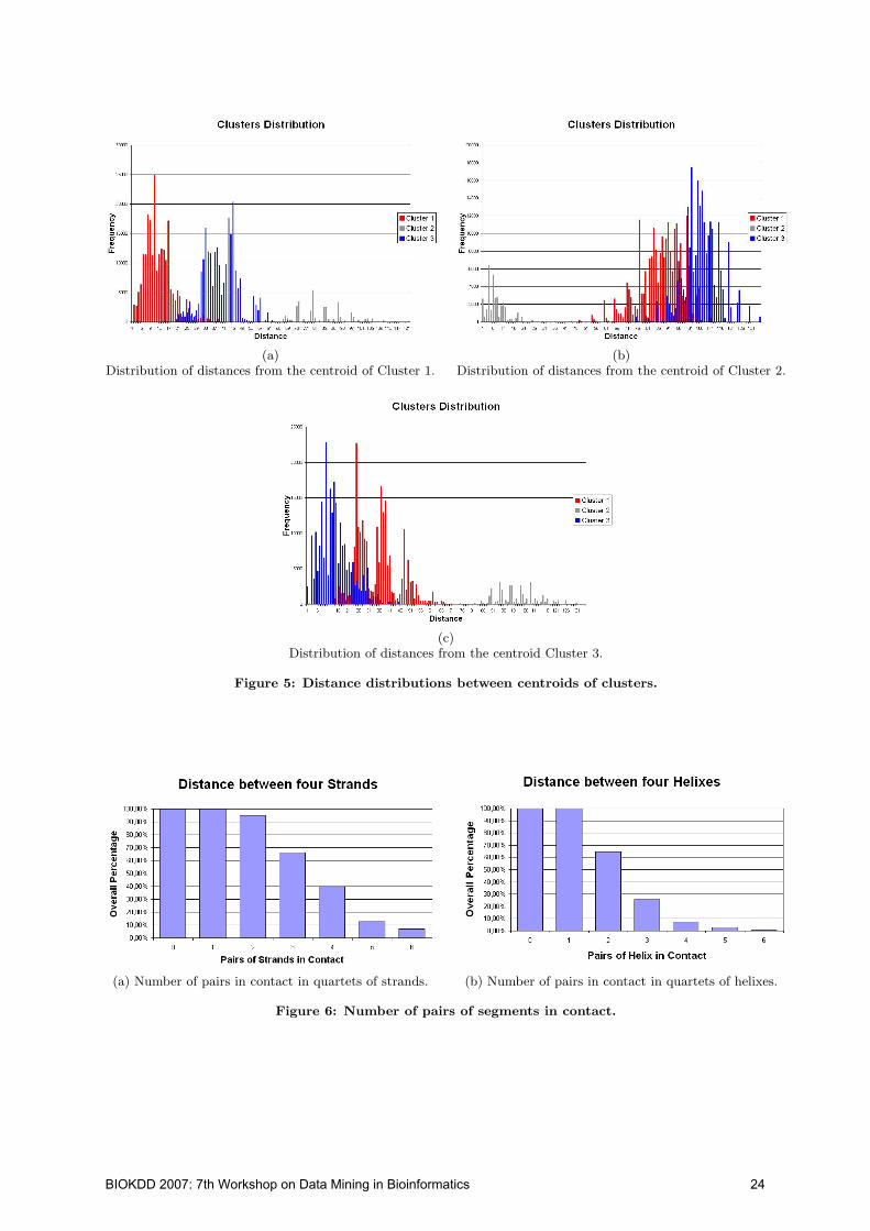
(a) (b)Distribution of distances from the centroid of Cluster 1. Distribution of distances from the centroid of Cluster 2.

(c)Distribution of distances from the centroid Cluster 3.

Figure 5: Distance distributions between centroids of clusters.

(a) Number of pairs in contact in quartets of strands. (b) Number of pairs in contact in quartets of helixes.

Figure 6: Number of pairs of segments in contact.


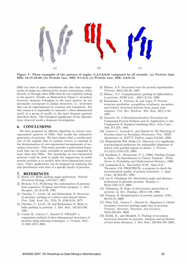
(a) (b) (c)

Figure 7: Three examples of the pattern of angles (1,2,7,8,8,9) composed by all strands: (a) Protein 1hpl,SSE: 16-17-18-20; (b) Protein 1acc, SSE: 0-1-2-3; (c) Protein 1aor, SSE: 4-6-8-12.

SSEs are close in space consolidates the idea that arrange-ments of angles are influenced by atomic interactions, eitherdirectly or through other SSEs that do not explicitly belongto the quartet. Finally, as illustrated in Figure 7, secondarystructure elements belonging to the same quartet do notnecessarily correspond to similar structures, i.e. structuresthat can be superimposed by rotation and translation. Forthis reason it is impossible to associate a three-dimensionalmotif, or a group of motifs, to the most frequent quartetsdescribed above. The biological significance of the distribu-tions observed needs a deepener investigation.

6. CONCLUSIONSWe have proposed an efficient algorithm to extract over-

represented quartets of SSEs, that avoids the exhaustivegeneration of patterns. We have shown that a careful anal-ysis of the angular bias of random vectors is essential inthe determination of over-represented arrangements of sec-ondary structures. This study provides a generalized frame-work that can be easily extended to patterns composed bymore than four SSEs. The knowledge of over-representedpatterns could be used to guide the engineering of stableprotein modules or to predict their three-dimensional struc-tures. Other applications can be designed by replacing thenull distribution with that of a specific family of proteins.

7. REFERENCES[1] Bowie J.U. Helix packing angle preferences. Natural

Structural Biology, 4:915-917, 1997.

[2] Brenner, S.A. Predicting the conformation of proteinsfrom sequences. Progress and future progress. J. Mol.Recognit., 8(1-2):9-28, 1995.

[3] Chothia, C., Levitt, M. and Richardson, D. Structureof proteins: packing of α-helices and pleated sheets.Proc. Natl. Acad. Sci., USA 74, 4130-4134, 1977.

[4] Chothia, C., Levitt, M. and Richardson, D. Helix tohelix packing in proteins. J. Mol. Biol., 145:215-250,1981.

[5] Comin M., Guerra C., Zanotti G. PROuST: acomparison method of three-dimensional structures ofproteins using indexing techniques. J. Comput. Biol.,11:1061-1072, 2004.

[6] Efimov, A.V. Structural trees for protein superfamilies.Proteins, 28(2):241-60, 1997.

[7] Efimov, A.V. Complementary packing of alpha-helicesin proteins. FEBS Lett. , 463(1-2):3-6, 1999.

[8] Eisenhaber, F., Persson, B. and Argos, P. Proteinstructure prediction: recognition of primary, secondary,and tertiary structural features from amino acidsequence. Crit. Rev. Biochem. Mol. Biol., 30(1):1-94,1995.

[9] Gerstein, M. A Resolution-Sensitive Procedure forComparing Protein Surfaces and its Application to theComparison of Antigen-Combining Sites. Acta Cryst. ,A48, 271-276, 1992.

[10] Guerra C., Lonardi S., and Zanotti G. 3D Matching ofProteins based on Secondary Structures. Proc. IEEESymposium on 3DPVT, Padova, pages 812-821, 2002.

[11] Hespenheide BM, Kuhn LA. Discovery of a significant,nontopological preference for antiparallel alignment ofhelices with parallel regions in sheets. 1: ProteinSci.12(5):1119-1125, 2003.

[12] Kaufman, L., Rousseeuw, P. J. (1990). Finding Groupsin Data - An Introduction to Cluster Analysis. WileySeries in Probability and Mathematical Statistics, 1990.

[13] Laskowski R.A., MacArthur M.W., Moss D.S.,Thornton J.M. PROCHECK: a program to check thestereochemical quality of protein structures. J. Appl.Cryst., 26:283-291, 1993.

[14] Lee S, Chirikjian GS. Interhelical angle and distancepreferences in globular proteins. Biophys J.,86(2):1105-1117, 2004.

[15] Nakamura, H. Roles of electrostatic interaction inproteins. Q. Rev. Biophys., 29(1):1-90, 1996.

[16] Persson, B. Bioinformatics in protein analysis. EXS.,88:215-31, 2000.

[17] Platt D.E., Guerra C., Zanotti G., Rigoutsos I. Globalsecondary structure packing angle bias in proteins.Proteins: Structure, Function, and Genetics,53(2):252-261, 2003.

[18] Reddy, B., and Blundell, T. Packing of secondarystructural elements in proteins. Analysis and predictionof inter-helix distances. J. Mol. Biol., 233:464-479, 2003.


[19] Walther, D., Eisenhaber, F. and Argos, P. Principlesof helix-helix packing in proteins: the helical latticesuperposition model. J. Mol. Biol., 255:536-553, 1996.

[20] Walther D, Springer C, Cohen FE. Helix-helix packingangle preferences for finite helix axes. Proteins,33(4):457-9, 1998.

[21] Yona G. and Kedem K. The URMS-RMS hybridalgorithm for fast and sensitive local protein structurealignment. Journal of Computational Biology, 12:12-32,2005.


Combining Domain Fusions and Domain-DomainInteractions to Predict Protein-Protein Interactions

Thanh Phuong NguyenSchool of Knowledge Science

Japan Advanced Institute of Science andTechnology

Ishikawa, [email protected]

Tu Bao HoSchool of Knowledge Science

Japan Advanced Institute of Science andTechnology

Ishikawa, [email protected]

ABSTRACTProtein-protein interactions are intrinsic to almost all cel-lular processes. Protein domains, the fundamental unitsin a protein are key elements to mediate such interactions.Whereas domain-based methods to predict protein-proteininteractions often used only protein domain information;protein-protein interactions, in fact, are also associated withthe biological nature of each interacting partner. Integrat-ing both protein domain features and genomic/proteomicfeatures of interacting partners is expected to better pre-dict protein-protein interactions, and to discover reciprocalbiological relationships among protein-protein interactions,protein domains, and genomic/proteomic features related toprotein-protein interactions.

We present a novel integrative domain-based approach forpredicting protein-protein interactions (PPI) using inductivelogic programming (ILP). Two principal domain featuresare domain fusions and domain-domain interactions. Var-ious relevant genomic and proteomic features of PPI are ex-ploited, from five popular genomic and proteomic databases.Integrating protein domain data and various kinds of datafrom multiple genomic and proteomic databases, we con-structed biologically significant ILP background knowledgeof nearly 220,000 ground facts. The experimental resultsfrom 10-fold cross-validation demonstrated that our approachcan better predict protein-protein interactions than othercomputational methods. When applied to many PPI datasets, our method can more reliably predict PPI in terms ofthe expression profile reliability indexes. The induced ILPrules give us a lot of interesting biological reciprocal relation-ships among protein-protein interactions, protein domains,and genomic/proteomic features related to protein-proteininteractions.

Supplementary materials are now available at http://www.jaist.ac.jp/∼s0560205/PPI/.

Permission to make digital or hard copies of all or part of this work forpersonal or classroom use is granted without fee provided that copies arenot made or distributed for profit or commercial advantage and that copiesbear this notice and the full citation on the first page. To copy otherwise, torepublish, to post on servers or to redistribute to lists, requires prior specificpermission and/or a fee.BIOKDD ’07, August 12, 2007, San Jose, California, USA.Copyright 2007 ACM 978-1-59593-839-8/07/0008 ...$5.00.

KeywordsProtein-protein interaction, Domain fusion, Domain-domaininteraction, Genomic/proteomic features, Inductive logic pro-gramming.

1. INTRODUCTIONProtein-protein interactions are indispensable at almost

every level of cell function, in the structure of sub-cellular or-ganelles, in the transport across the various biological mem-branes, in muscle contraction, signal transduction, and reg-ulation of gene expression, etc. Detecting protein func-tions via prediction of protein-protein interactions (PPI)has emerged as a new trend, both in vitro and in silico.Therefore, prediction of protein-protein interactions has be-come one of the most challenging tasks in the post-genomicera. Experimental techniques have marked unmistakableprogress in finding out and verifying protein interactions fordiverse organisms, including well-known ones such as two-hybrid assay [9], [28], affinity purification and mass spec-trometry [1], phage display [22]. Because of little overlapamong these experimental databases, the question abouttheir reliability is raised.

With the recent blooming of public proteomic and ge-nomic databases, numerous computational approaches offera chance to study more widely and deeply regarding protein-protein interactions. Depending on the source of informa-tion used, computational approaches can be categorized inthree groups: structure-based approach such as the workof [3], sequence-based approach such as the work of [14],and genome-based approach such as the work of [19]. Be-sides methods based on a single data source, many bioinfor-maticians make the effort to integrate multiple data sourcesto better predict PPI. Jansen et al. [10] used a Bayesiannetwork approach for integrating weakly predictive genomicfeatures into reliable predictions of protein-protein interac-tions. Several kernels for different data sources like pro-tein squences, Gene Ontology annotations, local propertiesof networks, etc. are combined to infer PPI [2]. Some otherefforts were the probabilistic decision tree approach [30], in-ductive logic programming method [25], probabilistic model[20], etc.

From multiple data sources, these works can extract andcombine various genomic and proteomic features related toPPI. The obtained results showed many advantages of mul-tiple data source integration. The shortcoming of their workis that they did not take protein domains into account.


However, it is a fact that the biological mechanism behindprotein-protein interactions involves protein domains andtheir interactions [18].

Protein domains are structural and/or functional unitsof proteins that are conserved through evolution to repre-sent protein structures or functions. They are believed tobe the key regulators in protein-protein interactions. In-teractions among domains are needed as stable channels ofPPI. Recently, prediction of PPI based on domains has re-ceived much attention in many ongoing studies. One of thepioneering works based on protein domains is an associa-tion method developed by Sprinzak and Margalit [23]. Kimet al. improved the association method by considering thenumber of domains in each protein [12]. Han et al. pro-posed a domain combination-based method by consideringthe possibility of domain combinations appearing in bothinteracting and non-interacting sets of protein pairs [8]. Agraph-oriented method is proposed by Wojcik and Schachtercalled the interacting domain profile pairs (IDPP) method[29]. Chen et al. used domain-based random forest frame-work to predict PPI [4].

The previous work all treasured the biological roles of pro-tein domains in PPI prediction. The main disadvantageof these methods is that most of them merely consideredthe co-occurrence of domains/domain pairs. To predict PPIcomprehensively, it is necessary to combine various domainfeatures and genomic/proteomic features.

In this paper, we present a novel integrative domain-basedapproach using inductive logic programming to predict pro-tein-protein interactions. The key idea of our computationalmethod is to integrate protein domain features and multi-ple genomic and proteomic features. To combine efficientlyboth features of protein domains and different features ofgenomes and proteomes to predict PPI, we specified twomain tasks. The first one is extracting as many useful do-main and genomic/proteomic features as possible relatedto PPI. From seven popular databases, we extracted morethan two hundred thousand ground facts of domain fusion,domain-domain interaction features and various other bio-logically significant genomic/proteomic features. The sec-ond one is employing inductive logic programming (ILP)with the huge amount of background knowledge to effec-tively infer PPI.

To demonstrate the advantages of the integration domainfeatures and genomic/proteomic features in PPI prediction,we conducted 10-fold cross validation tests for our methodsand two other methods based on single domain features,and also for the non domain-based approach using multi-ple genomic databases. For all cases, our method performedconsiderably better than others. The expression profile reli-ability index (EPR Index) additionally showed the high reli-ability of our methods when applied to several PPI datasets.At last, analyzing various produced rules, many interestingrelationships among PPI and DDI, and protein functions,biological processes were found. Our proposed methods canbe tuned to predict PPI for diverse organisms and othergenomic and proteomic data sources.

The remainder of the paper is organized as follows. InSection 2, we present our proposed method to predict PPIbased on domains using ILP and multiple genomic and pro-teomic databases. The comparative evaluation of the exper-iments is given in Section 3. Predictive rules of PPI, as wellas discussion, are presented in Section 4. Some concluding

remarks are given in Section 5.

2. MATERIALS AND METHODSIn this section, we present our proposed method to predict

protein-protein interactions based on domain and multiplegenomic and proteomic data using ILP. Two main tasks ofthe method are: (1) Constructing integrated backgroundknowledge1 of domain features and multiple genomic andproteomic features, and (2) Learning PPI predictive rulesby ILP from the constructed background knowledge. Con-structing ILP background knowledge requires two steps. Thefirst one is defining ILP predicates. The second one is ex-tracting ground facts2 to define extensionally predicates.

When choosing a feature, we concentrated on two points.First is the biological role of that feature in protein-proteininteractions or domain-domain interactions, and second isthe availability of data of that feature. Based on results ofexperimental and computational research on PPI, twentytwo features of protein domains and genomes/proteomeswere chosen and were formulated using ILP predicates. Thehuge database of more than 220,000 ground facts of twentytwo predicates is sufficient for accurate PPI prediction.

We first introduce briefly about Inductive Logic Program-ming (ILP) and some bioinformatic applications of ILP inSection 2.1. Then the first task in our proposed method ispresented in Subsections 2.2, 2.3, and 2.4. Subsection 2.5describes the second task.

2.1 Inductive Logic ProgrammingInductive Logic Programming is the intersection of ma-

chine learning and logic programming [15]. ILP aims to de-velop theories, techniques, and tools for inducing hypothesesfrom observations using representations from computationallogic. ILP studies learning from examples, within the frame-work provided by clausal logic. Here the examples and back-ground knowledge are given as clauses, and the theory thatis to be induced from these, is also to consist of clauses.

An ILP system is generally set with three languages:LO : the language of observationsLB : the language of background knowledgeLH : the language of hypotheses

Given a consistent set of examples of observations O ⊆ LO

and consistent background knowledge B ⊆ LB, ILP systemsfind hypotheses H ∈ LH such that:

B ∧H ` O

Distinguishing features of ILP are its ability to take intoaccount background (domain) knowledge in the form of logicprograms, and the expressive power of the language of dis-covered patterns [7]. ILP is particular suitable for bioin-formatics tasks because of its ability to take into accountbackground knowledge and work directly with structureddata. The ILP system GOLEM has been applied to findthe predictive theory about the relationship between chem-ical structure and activity, eg. the problem of inhibitionof E.Coli Dihydrofolate Reductase by two different groupsof drugs (pyrimidines and triazines) [13]. Other central con-cerns of bioinformatics have been convincingly solved by ILP

1the term ’background knowledge’ is used here in terms ofthe language of inductive logic programming.2the term ’ground facts’ is used here in terms of the languageof inductive logic programming.


, such as protein secondary structure prediction [16], proteinfold recognition [27], etc.

2.2 Extracting Domain Fusion and Domain-Domain Interaction Data

Protein domains form the structural or functional unitsof proteins that partake in intermolecular interactions. Theexistence of certain domains in proteins can therefore sug-gest the propensity for the proteins to interact or form astable complex to bring about certain biological functions.Domain fusion and domain-domain interaction features haveimportant biological roles in PPI prediction [26], [18], andthese two domain features are extracted in our work.

Let P denote the set of considered proteins pi. Denote byD the set of all protein domains dk which belong to proteinspi. A protein pair (pi, pj) that interacts together is denotedby pij , and a protein pair that does not interact together by¬pij . Similarly for a domain pair (dk, dl), dkl represents aninteraction, and ¬dkl a non-interaction.

Domains of interacting proteins have more chance to fusetogether than domains of non-interacting proteins. There-fore, when finding a pair of proteins which have fused do-mains, we can predict an interaction between them. Domainfusion data is referred from Domain Fusion Database [26].We extracted domain fusion data for protein pairs (pi, pj),∀pi, pj ∈ P . The following predicate represents the domainfusion between two proteins:

domain fusion(+protein, +protein, #FUSION) (1)

Note that in the ILP system used - system Aleph (A learn-ing engine for proposing hypothesis) [24], there are somemode declarations to build the bottom clauses, and a sim-ple mode type is one of the following: (1) the input vari-able (+), (2) the output variable (−), or (3) the constantterm (#). Predicate (1) means whether two input pro-teins, A and B, have fused domains or not (valued ”yes”by the constant term #FUSION). This predicate is supportedby a set of ground facts Gdomain fusion, e.g., domain fusion(ap3m yeast, ap3b yeast, yes). After preprocessing, the setGdomain fusion consists of 255 ground facts for protein pairs.

The assumption that proteins interact with each otherthrough interactions of their domains is widely acceptedand validated. The domain-domain interaction data is ex-ploited to more reliably predict PPI. We extracted DDI datafrom iPfam database (http://www.sanger.ac.uk/Software/Pfam/iPfam/). iPfam is a resource that describes domain-domain interactions that are observed in PDB entries. Thedomains are defined by Pfam. When two or more domainsoccur in a single structure, the domains are analysed to seeif they form an interaction considered by the bonds formingthe interaction are calculated.

We considered two features of DDI. The first feature iswhether a protein pair (pi, pj) has a domain interaction dkl,and if yes, how many dkl it has. This information is formu-lated by predicate:

hasddi(+protein, +protein, #DDI) (2)

The set of ground facts for this predicate Gddi includes 573ground facts, some of them are: hasddi(jsn1 yeast,yip1 yeast,2), hasddi(msh4 yeast,msh5 yeast,5), etc.

The number of domain-domain interactions of a proteinis one of the features which may increase or decrease theprobability of its interaction with others. So we considered

the relationship between PPI and the number of DDI ofeach interacting partner. This relationship is presented inpredicate 3.

num ddi(+protein, #NUM DDI) (3)

Denoted by Gnum ddi, the set of ground facts of the abovepredicate contains 289 ground facts. We found that thereare some proteins having a large number of DDI, for exam-ple num ddi(did4 yeast,20) or num ddi(bud27 yeast,39), andthese proteins potentially interact with many other proteins.

2.3 Extracting Proteomic and Genomic Datafrom Multiple Databases

In addition to domain fusion and domain-domain inter-action features as shown in the previous section, we minedgenomic and proteomic data from UniProt database, CYGDdatabase, InterPro database, Gene Ontology database, andGene Expression database to detect useful genomic and pro-teomic features for PPI prediction.

As the world’s most comprehensive catalog of informa-tion on proteins, UniProt database (http://www.pir.uni-prot.org/) largely provides functional, structural or othercategories (in Keyword - KW line); regions or sites of inter-est in the sequences (in Feature Table - FT lines); describesenzymes coded (EC) and pointers to information related toentries and found in data collections other than Uniprotsuch as GO database, PIR database, PROSITE database,Pfam database, and Interpro database (in Database cross-Reference - DR line). There are the following predicates foreach kind of information for one protein.

keyword(+protein, #KW) (4)

feature(+protein, #FT) (5)

coded enzyme(+protein, #EC) (6)

dr go(+protein, −GO TERM) (7)

dr pir(+protein, −PIR ID) (8)

dr prosite(+protein, −PROTSITE ID) (9)

dr pfam(+protein, −PFAM ID) (10)

dr interpro(+protein, −INTERPRO ID) (11)

For example, some extracted data for these predicatesare keyword(ace1 yeast,transcription regulation), feature(ldb7yeast, chain chromatin structure remodeling complex), codedenzyme(uqcr1 yeast, ec1.10.2), and dr go(twoa5d yeast,

go0005935), etc. The first three predicates present generalprotein features that should effect their interactions. Theother give references to other databases. Data from differ-ent databases related to PPI are bound by these predicates.We extracted 10,919 ground facts for these UniProt predi-cates.

The MIPS Comprehensive Yeast Genome DatabaseCYGD (http://mips.gsf.de/genre/proj/ yeast/) aims topresent information on the molecular structure and func-tional network of the entirely sequenced, well-studied modeleukaryote, the budding yeast Saccharomyces cerevisiae.

Among various information provided by CYGD, cataloguesof functions, catalogues of subcellular locations, cataloguesof phenotypes, catalogues of complexes, and catalogues ofproteins should be mined to discover the biological relation-ship between such catalogues and protein-protein interac-tions. Also, proteins in the same catalogue have more chanceto interact together than other proteins. The set of groundfacts extracted from CYGD database GCY GD consists of


2,152 ground facts. Here are some examples: subcell cat(ahc1 yeast, cytoplasm), phenotype cat(cyk2 yeast, cell cycledefects), etc.

function cat(+protein, #FUNCAT) (12)

subcell cat(+protein, #SUBCELLCAT) (13)

phenotype cat(+protein, #FENCAT) (14)

complex cat(+protein, #COMPLEXCAT) (15)

protein cat(+protein, #PROTEINCAT) (16)

InterPro database (http://www.ebi.ac.uk/interpro/) isa database of protein families, domains and functional sitesin which identifiable features found in known proteins canbe applied to unknown protein sequences. We consideredthe association between InterPro identifers and GO terms.There are 556 ground facts which support this predicate.

interpro go(+INTERPRO ID, −GO TERM) (17)

Gene Ontology database (http://www.geneontology.org)has three organizing principles: molecular function, bio-logical process and cellular component. The terms in anontology are linked by two relationships, is a and part of.The relationships of interacting partners in a PPI may ef-fect their interaction. Predicates 18, 19, having 438 groundfacts (e.g., is a (go0000002, go0007005), part of (go0000032,go0007047)) show these relationships:

is a(+GO TERM, −GO TERM) (18)

part of(+GO TERM, −GO TERM) (19)

Proteins in the same complex are often co-expressed, andthen this genomic feature is useful in predicting PPI. Thegene expression coefficients referred to in [10] betweentwo proteins are presented in the following predicate (having200,000 ground facts):

expression(+protein, +protein, #COEFFICIENT) (20)

Two last predicates express information about the num-ber of protein-protein interactions (with 690 ground facts)and interaction generality of two interacting partners (with1,718 ground facts). Interaction generality is the number ofproteins that interact with both interacting partners.

num ppi(+protein, +protein, #NUM PPI) (21)

ig(+protein, +protein, #IG) (22)

2.4 Constructing Background Knowledge forPredicting Protein-Protein Interactions

After twenty two predicates are defined, data in terms ofground facts for these predicates are next exploited fromseven databases (two databases for domain features and fiveothers for genomic and proteomic features). In succession,we denote the sets of ground facts extracted from UniProtdatabase, CYGD database, InterPro database, Gene Ontol-ogy database, and Gene Expression database by GUniProt,GGO, GInterPro, GCY GD, and Gexpression. Algorithm 1presents the procedure to extract data from multipledatabases to construct background knowledge for PPI pre-diction.

Algorithm 1 Extracting domain and protein data frommultiple sources.

Input:Set of proteins P ⊃ {pi}.

Output:Sets of ground facts Gdomain fusion, Gddi, Gnum ddi,GUniProt, GCY GD, GInterPro, GGO, , Gexpression, Gig,and Gnum ppi.

1: Initialize all sets of ground facts GL := ∅ (∀ GL ∈Gdomain fusion, Gddi, Gnum ddi, GUniProt, GCY GD,GInterPro, GGO, , Gexpression, Gig, and Gnum ppi);D := ∅.

2: Extract all domains dk belonging to proteins pi;D := D ∪ {dk}.

3: for each protein pair (pi, pj)4: for all dk ∈ pi and dl ∈ pj

5: if fused(dk, dl) = true thenGdomain fusion := Gdomain fusion ∪ {(pi, pj)}

6: if ∃ dkl thenGddi := Gddi ∪ {(pi, pj)}Count the number of DDI num ddii andnum ddij for proteins pi, and pj respectively;

7: Gnum ddi := Gnum ddi ∪ {(pi, num ddii)}∪{(pj , num ddij)}.

8: for each protein pi ∈ P9: Extract data from UniProt database and CYGD

database for GUniProt and GCY GD respectively;GUniProt = GUniProt ∪ {pi, pi.data};GCY GD = GCY GD ∪ {pi, pi.data}.

10: Extract mapping data between GO terms gi andInterpro identifiers ti related to pi from InterProdatabase for GInterpro;GInterPro = GInterPro ∪ {ti, gi.}.

11: for each protein pi ∈ P12: for each protein pj ∈ P13: Extract the relationship rij between GO terms

(gi, gj) related to (pi, pj) from GO database;GGO = GGO ∪ {rij(gi, gj)}.

14: Extract the expression correlation coefficients eij of(pi, pj);Gexpression = Gexpression ∪ {pi, pj , eij}

15: Extract the interaction generality of PPI nij of(pi, pj); Gig = Gig ∪ {pi, pj , nij}

16: if ∃ pij thennum ppii := num ppii + 1;

17: Gnum ppi := Gnum ppi ∪ {(pi, num ppii)}.18: return Gdomain fusion, Gddi, Gnum ddi, GUniProt,

GCY GD, GInterPro, GGO, , Gexpression, Gig, Gnum ppi.

2.5 PredictingProtein-Protein Interaction Us-ing Inductive Logic Programming

The proposed integrative domain-based ILP frameworkfor predicting PPIs from multiple genomic and proteomicdatabases is described in Algorithm 2.

The previous framework presents the common proceduresof the ILP method. Step 2 and Step 3 are for generatingpositive and negative examples Sinteract, S¬interact respec-tively (see more Subsection 3.1). In Step 4, we extractedbackground knowledge Sbackground including both domainfeatures and genomic and proteomic features from sets ofground facts of defined predicates (see Section 2.4). In Step5, in our experiments, system Aleph was applied to inducerules. Aleph is an advanced ILP system that uses a top-down ILP covering algorithm.

Aleph requires three input files to construct theories: pos-itive examples, negative examples and background knowl-edge. Positive and negative examples can simply be consid-


Algorithm 2 An integrative domain-based ILP frameworkfor PPI prediction

Input:Set of protein-protein interactions Sinteract ⊃ {pij}Number of negative examples (¬pij) NSets of ground facts Gdomain fusion, Gddi, Gnum ddi,GUniProt, GCY GD, GInterPro, GGO, , Gexpression, Gig,and Gnum ppi.

Output:Set of rules R for protein-protein interaction prediction.

1: R := ∅.2: Extract positive examples for the set Sinteract.3: Generate N negative examples ¬pijs by selecting N pro-

tein pairs (pi, pj) where pi, pj ∈ P and pi, pj are locatedin different subcellular compartments;S¬interact = {¬pij}.

4: call Algorithm 1 to generate sets of ground facts GL

and Sbackground =⋃

GL (∀ GL ∈ Gdomain fusion,Gddi, Gnum ddi, GUniProt, GCY GD, GInterPro, GGO, ,Gexpression, Gig, and Gnum ppi.

5: Run an ILP program with Sinteract, S¬interact andSbackground to induce rules r.

6: R := R ∪ {r}.7: return R.

ered as ground facts. Background knowledge is in the formof Prolog clauses that encode information relevant to thedomain. All predicates appearing in hypothesized clauseshave to be declared, and amongst them the target predicateis learned to induce rules. The target predicate in our workis: has_int(+protein, +protein), meaning that two arbi-trary proteins, A and B, interact. Aleph learns three inputsand induces rules (hypothesized clauses) in terms of the rela-tionships between the target predicate and other predicatesdeclared in background knowledge.

3. EXPERIMENTAL RESULTS

3.1 Experiment DesignWe concentrate on predicting PPI for Saccharomyces cere-

visiae, a budding yeast, due to the availability of Saccha-romyces cerevisiae data. We carried out experimental com-parative evaluation for protein-protein interaction predic-tion.

To assess the performance of our method for PPI predic-tion, we did three comparative tests to demonstrate: (1) theadvantages of the integration of multiple proteomic and ge-nomic features in our method, (2) the advantages of domain-based approach, and (3) the reliability of our method. First,ROC curves of 10-fold cross validation tests were producedto compare our proposed method with other domain-basedmethods, particularly AM method and SVMs method. Sec-ond, we also conducted 10-fold cross validation tests for anILP method with multiple genomic databases, but not us-ing domain features, and compared those results with ourmethod in terms of sensitivity and specificity. At last, apply-ing our method to several PPI datasets like Ito dataset [9],Uetz dataset [28], MIPS dataset (http://mips.gsf.de/proj/ppi/), DIP dataset (http://dip.doe-mbi.ucla.edu/), etc., weestimated EPR indexes [5] to show the reliability of ourmethod.

For three comparative tests for PPI prediction, we used

the core data of Ito data set [9] with more than two IST hits3,as positive examples, and selected at random 1000 proteinpairs whose elements are in separate subcellular compart-ments as negative examples. Each interaction in the inter-action data originally shows a pair of bait and prey ORF(Open Reading Frame). After removing all interactions inwhich either bait ORF or prey ORF is not found in UniProtdatabase, we obtained 718 interacting pairs from the origi-nal 841 pairs. Subsection 3.2 shows the experimental resultsof PPI prediction.

3.2 Predicting Protein-Protein InteractionsWith the same positives and negatives datasets, we con-

ducted 10-fold cross validation tests for our method, AMmethod and SVMs method. AM method calculated theprobability of protein pairs based on protein domains [23].In our experiment, the probability threshold is set to 0.05.For SVMs method, we used SV M light [11]. The linear ker-nel with default values of the parameters was used. ForAleph, we selected minpos = 2 and noise = 0, i.e. the lowerbound on the number of positive examples to be covered byan acceptable clause is 2, and there are no negative examplesallowed to be covered by an acceptable clause. We also usedthe default evaluation function coverage which is defined asP −N , where P , N are the number of positive and negativeexamples covered by the clause.

Figure 1: Comparative ROC curves of ILP, SVMsand AM method with 1000 negative examples.

The ROC curves of ILP, AM and SVMs methods with1000 negative examples are shown in Figure 1. ROC curve(Receiver Operating Characteristic curve) shows the trade-off between sensitivity and specificity (any increase in sen-sitivity will be accompanied by a decrease in specificity).Sensitivity refers to the ability of the test to detect individ-uals who actually have the disorder. On the other hand, theterm specificity means that the test is specific to the disor-der being assessed and that it does not give a positive resultbecause of other conditions.

The ROC curve of our method is close to the left-handborder and then the top border of the ROC space. On theother hand, ROC curves of AM method and SVMs methodare close to the 45-degree diagonal of the ROC space. TheROC curve demonstrates that our method has a consid-

3IST hit means how many times the corresponding interac-tion was observed. The higher the IST number, the morereliable the corresponding interaction is.


Table 1: Evaluation of our proposed method using EPR index with Ito, Uetz, Ito+Uetz, MIPS, and DIP PPIdatasets.

Data Number of interactions EPR indexOriginal Our proposed Original Proposed

Ito 4549 2000 0.191 ± .0306 0.349 ± .0491Uetz 1474 799 0.445 ± .0588 0.539 ± .0831

Ito+Uetz 5827 2699 0.238 ± .0287 0.363 ± .0437MIPS 14146 6810 0.595 ± .0337 0.685 ± .0422DIP 15409 9047 0.418 ± .0260 0.541 ± .0371

Figure 2: The sensitivity and specificity (denote bySensitivity1 and Specificity1) of non-domain basedapproach are compared with those (denote by Sen-sitivity2 and Specificity2) of our proposed methodwith various sets of negative examples by 10-foldcross-validation tests.

erably better performance than those of AM and SVMsmethod.

Conducting 10-fold cross-validation with various testednumbers of negative examples, the results (in Figure 2) showthat our method achieved higher sensitivity, and higher orequal specificity, than the non-domain based approach [25].

To show how reliable our method is, we compared theEPR indexes of original PPI datasets and datasets predictedby our method. The EPR index estimates the biologicallyrelevant fraction of protein interactions detected in a highthroughput screen. For each given dataset, we first excludedall protein pairs which overlap with those in the trainingdataset. All retrieved protein pairs that classified as posi-tives are then estimated in terms of their EPR indexes. Ta-ble 1 shows the higher ERP index of our method comparedwith original ones.

4. DISCUSSIONThe experimental results have shown that ILP approach

potentially predicts PPI and DDI with high sensitivity andspecificity. Furthermore, the inductive rules of ILP encour-aged us to discover many interesting biological reciprocal re-lationships among protein-protein interactions and proteindomains, and other genomic/proteomic features related toprotein-protein interactions. Analysing our results in com-parison with information in biological literatures and books,we found that ILP induced rules could be applied to furtherrelated studies in biology.

Studying the rules of PPI prediction related to domain-domain interaction information, we found many interestingrules. For example, the following rule shows that if twoproteins have domains belonging to domain databases likePROSITE database or InterPro database and these domainsinteract with each other, they may interact.

has int (A,B) :- dr prosite (B, C), dr prosite (A, C),ddi (A, B, yes) with 43 positives covered

has int(A,B) :- dr interpro(B,C), dr interpro(A,C), ddi(A, B, yes)with 90 positives covered.

A large number of positives, which indicates these rules,confirms why domain-domain interactions are considered askey factors to predict PPI.

Considering the group of proteins which may be requiredfor the production of pyridoxine (vitamin B6) sno1 yeast,snz3 yeast snz1 yeast, and snz2 yeast, we found that eachpair in this group has an interaction which satisfies the fol-lowing rule:

has int(A,B) :- ig (A, B, C), C = 1, ddi (A, B, yes),function cat (B, cell rescue defense and virulence).

This rule means interaction of protein A and protein Bmay occur if the proteins satisfy three conditions. First isthat they interact with the same protein. Second is that theyhave at least one DDI. Third is that one of them is catego-rized to function catalogue cell rescue defense and virulence.We knows that PPI play an important role in drug design,so such rules and their evidence, are expected to help usto discover interesting relationships between PPI, DDI andprotein function in pharmaceuticals.

Two most popular rules related to domain fusion informa-tion are:

has int(A,B) :- dr go(B,C), part of(C,D), domain fu-sion(A,B,yes)

has int(A,B) :- dr go(B,C), dr go(A,C), domain fu-sion(A,B,yes)

The first one covers 199 positives and the second one cov-ers 217 positives. Both of these rules consist of GO termsand domain fusion information. According to the secondrule, if two proteins have GO terms and their domains arefused in another protein, there may occur an interaction.

Our induced rules with large number of positives provethat if a pair of proteins, A and B, are located in the samesubcellular compartment, protein A potentially interacts withprotein B. In case of nucleus compartment, there are 216 cov-ered positives, 284 for cytoplasm compartment and 15 formitochondria compartment. However, surprisingly amonginduced rules, we found a rule with 37 positives that showedthe phenomenon of two proteins being in different subcellu-lar locations but interacting.

has int(A,B) :- subcell cat(B,nucleus), subcell cat(A, cy-toplasm), function cat(A,transcription).


This phenomenon could occur when there is a certaintranslocation or post-translation modification of proteins indifferent subcellular compartments.

Since protein-protein interactions have close biological as-sociations with domain-domain interactions, discovering DDIfrom PPI data is an area of much ongoing research. Nget al. proposed to an integrative approach to infer puta-tive domain-domain interactions from three data sources,including experimentally-derived protein interactions, pro-tein complexes and Rosetta stone sequences [17]. To predictDDI, the maximum likelihood estimation (MLE) is appliedby Deng et al. [6]. Riley et al. proposed a domain pair ex-clusion analysis (DPEA) for predicting DDI from databasesof protein interactions [21]. These works showed that DDIcan be efficiently predicted from PPI data. In the future, asmore DDI are predicted and validated, our work is potentialto reliably predict PPI. From PPI networks, we can build upmore complex protein complexes and pathways in cell, suchas signal transduction pathways or metabolic pathways.

5. CONCLUSIONWe have presented an integrative domain-based approach

using ILP and multiple genome databases to predict protein-protein interactions. The experimental results demonstratedthat our proposed method could produce comprehensiblerules, and at the same time, performed well in comparisonwith other work on protein-protein interaction prediction.In future work, we would like to investigate induced rules tostudy further the biological relationships among PPI, DDI,domain fusion and other genomic/proteomic features. Inte-grating more biological features may achieve better results.We also would like to apply the ILP approach to other im-portant tasks, such as determining protein functions, anddetermining the sites, and interfaces of PPI using DDI data.

6. REFERENCES[1] A. Bauer and B. Kuster. Affinity purification-mass

spectrometry: Powerful tools for the characterizationof protein complexes. Eur. J. Biochem.,270(4):570–578, 2003.

[2] A. Ben-Hur and W. S. Noble. Kernel methods forpredicting protein-protein interactions.Bioinformatics, 21(suppl1):i38–46, 2005.

[3] J. R. Bock and D. A. Gough. Predictingprotein-protein interactions from primary structure.Bioinformatics, 17(5):455–460, 2001.

[4] X. Chen and M. Liu. Prediction of protein-proteininteractions using random decision forest framework.Bioinformatics, 21(24):4394–4400, 2005.

[5] C. M. Deane, L. Salwinski, I. Xenarios, andD. Eisenberg. Protein interactions: Two methods forassessment of the reliability of high-throughputobservations. Mol Cell Proteomics, pagesM100037–MCP200, 2002.

[6] M. Deng, S. Mehta, F. Sun, and T. Chen. Inferringdomain-domain interactions from protein-proteininteractions. Genome Res., 12(10):1540–1548, 2002.

[7] S. Dzeroski and N. Lavrac, editors. Relational DataMining. Springer, 2001.

[8] D. Han, H.S.Kim, J.Seo, and W.Jang. A domaincombination based probabilistic framework for

protein-protein interaction prediction. In GenomeInformatics, pages 250–259, 2003.

[9] T. Ito, T. Chiba, R. Ozawa, M. Yoshida, M. Hattori,and Y. Sakaki. A comprehensive two-hybrid analysisto explore the yeast protein interactome. In Proc.Natl. Acad. Sci. USA 98, pages 4569–4574, 2001.

[10] R. Jansen, H. Yu, D. Greenbaum, Y. Kluger, N. J.Krogan, S. Chung, A. Emili, M. Snyder, J. F.Greenblatt, and M. Gerstein. A Bayesian NetworksApproach for Predicting Protein-Protein Interactionsfrom Genomic Data. Science, 302(5644):449–453, 2003.

[11] T. Joachims. Making large-scale support vectormachine learning practical. In B. Scholkopf,C. Burges, and A. Smola, editors, Advances in KernelMethods: Support Vector Machines. MIT Press,Cambridge, MA, 1998.

[12] R. Kim, J. Park, and J. Suh. Large scale statisticalprediction of protein - protein interaction bypotentially interacting domain (PID) pair. In GenomeInform. Ser. Workshop Genome Inform, pages 48–50,2002.

[13] R. King, S. Muggleton, R. Lewis, and M. Sternberg.Drug design by machine learning: The use of inductivelogic programming to model the structure activityrelationships of trimethoprim analogues binding todihydrofolate reductase. Proc. of the NationalAcademy of Sciences of the USA, 89(23):11322–11326,1992.

[14] L. R. Matthews, P. Vaglio, and J. R. et al.Identification of potential interaction networks usingsequence-based searches for conserved protein-proteininteractions or ’interologs’. Genome Res.,11(12):2120–2126, 2001.

[15] S. Muggleton. Inductive Logic Programming.Academic Press, 1992.

[16] S. Muggleton, R. King, and M. Sternberg. Proteinsecondary structure prediction using logic-basedmachine learning. Protein Eng., 6(5):549–, 1993.

[17] S. Ng, Z. Zhang, and S. Tan. Integrative approach forcomputationally inferring protein domain interactions.Bioinformatics, 19(8):923–929, 2003.

[18] T. Pawson, M. Raina, and N. Nash. Interactiondomains: from simple binding events to complexcellular behavior. FEBS Letters, 513(1):2–10, 2002.

[19] M. Pellegrini, E. M. Marcotte, and M. J. T. et al.Assigning protein functions by comparative genomeanalysis: Protein phylogenetic profiles. In Proc. Natl.Acad. Sci. USA, volume 96, pages 4285–4288, 1999.

[20] D. R. Rhodes, S. A. Tomlins, S. Varambally,V. Mahavisno, T. Barrette, S. Kalyana-Sundaram,D. Ghosh, A. Pandey, and A. M. Chinnaiyan.Probabilistic model of the human protein-proteininteraction network. Nat Biotech, 23(8):1087–0156,2005.

[21] R. Riley, C. Lee, C. Sabatti, and D. Eisenberg.Inferring protein domain interactions from databasesof interacting proteins . Genome Biology, 6(10):R89,2005.

[22] G. P. Smith. Filamentous fusion phage: Novelexpression vectors that display cloned antigens on thevirion surface. Science, 228(4705):1315–1317, 1985.

[23] E. Sprinzak and H. Margalit. Correlated


sequence-signatures as markers of protein-proteininteraction. Journal of Molecular Biology,311(4):681–692, 2001.

[24] A. Srinivasan, 1993.http://web.comlab.ox.ac.uk/oucl/research/areas/machlearn/Aleph/.

[25] T. Tran, K.Satou, and T.B.Ho. Using inductive logicprogramming for predicting protein-proteininteractions from multiple genomic data. In PKDD’05,pages 321–330, 2005.

[26] K. Truong and M. Ikura. Domain fusion analysis byapplying relational algebra to protein sequence anddomain databases. BMC Bioinformatics, 4(16):1–10,2003.

[27] M. Turcotte, S. Muggleton, and M. Sternberg. Proteinfold recognition. In Proc. of the 8th InternationalWorkshop on Inductive Logic Programming (ILP-98),pages 53–64, 1998.

[28] P. Uetz, L. Giot, G. Cagney, T. A. Mansfield, R. S.Judson, J. R. Knight, D. Lockshon, V. Narayan,M. Srinivasan, P. Pochart, A. Qureshi-Emili, Y. Li,B. Godwin, D. Conover, T. Kalbfleisch,G. Vijayadamodar, M. Yang, M. Johnston, S. Fields,and J. M. Rothberg. A comprehensive analysis ofprotein-protein interactions in saccharomycescerevisiae. Nature, 403(6770):623–627, February 2000.

[29] J. Wojcik and V. Schachter. Protein-proteininteraction map inference using interacting domainprofile pairs. Bioinformatics, 17(suppl1):S296–305,2001.

[30] L. Zhang, S. Wong, O. King, and F. Roth. Predictingco-complexed protein pairs using genomic andproteomic data integration. BMC Bioinformatics,5(38), 2004.


A Linear-time Algorithm for Predicting FunctionalAnnotations from Protein Protein Interaction Networks∗

Yonghui WuDepartment of Computer Science & Engineering

University of CaliforniaRiverside, CA 92507

[email protected]

Stefano Lonardi∗

Department of Computer Science & EngineeringUniversity of CaliforniaRiverside, CA [email protected]

ABSTRACTRecent proteome-wide screening efforts have made availablegenome-wide, high-throughput protein-protein interaction(PPI) maps for several model organisms. This has enabledthe systematic analysis of PPI networks, which has becomeone of the primary challenges for the system biology com-munity. Here we address the problem of predicting the func-tional classes of proteins (i.e., GO annotations) based solelyon the structure of the PPI network. We present a maximumlikelihood formulation of the problem and the correspondinglearning and inference algorithms. The time complexity ofboth algorithms is linear in the size of the PPI network andexperimental results show that their accuracy in the func-tional prediction outperforms current existing methods.

1. INTRODUCTIONHigh-throughput protein-protein interaction (PPI) net-

works with various levels of proteome coverage are currentlyavailable for several model organisms, namely S. cerevisiae

[19], D. melanogaster [7, 6], C.elegans [12], H. sapiens [15]and H. pylori [14]. PPI data can be obtained through avariety of sophisticated assays, like co-immunoprecipitation,yeast two hybrid, tandem affinity purification and mass spec-trometry. A PPI network is usually represented by a node-labeled undirected graph where vertices correspond to pro-teins and edges denote physical interactions.

Since the main mechanism by which cells are able to pro-cess information is through protein-protein interactions, PPIdata has been essential to obtain new knowledge and insightsin a wide spectrum of biological processes. In this paper, wefocus on the problem of predicting the functional categoryof proteins solely based on the topological structure of thePPI network. The rationale of this approach is based on theobservation that a protein is much more likely to interactwith another protein in the same functional class than with

∗This project was supported in part by NSF CAREER IIS-0447773, and NSF DBI-0321756.∗Corresponding author

Permission to make digital or hard copies of all or part of this work forpersonal or classroom use is granted without fee provided that copies arenot made or distributed for profit or commercial advantage and that copiesbear this notice and the full citation on the first page. To copy otherwise, torepublish, to post on servers or to redistribute to lists, requires prior specificpermission and/or a fee.BIOKDD’07 , August 12, 2007, San Jose, California, USACopyright 2007 ACM 978-1-59593-839-8/07/0008 ...$5.00.

a protein with a different function (see, e.g., [10, 21, 18, 13]).The prediction of functional classes can be useful either forproteins for which there is little or non-existing functionalinformation (e.g., for predicting the involvement of a proteinin specific pathway), or to confirm existing annotations pro-vided by other methods. Motivated by the expectation thatin the near future massive PPI networks will be available,here we propose a computationally efficient method that ac-curately determines the functional categories and will becapable to scale gracefully with the size of the network.

A variety of algorithmic techniques have been proposed inthe literature to solve the problem of functional predictionwith a wide range of computational complexity. Perhapsthe most computationally efficient algorithm is based onthe majority rule where the function of an unknown proteinis simply determined by the most common function amongits interacting partners [17]. A slightly more sophisticatedmajority-based method is the χ2-method proposed in [8]. Atthe other end of the computational complexity spectrum, theauthors of [21, 10] propose to assign proteins to functionalclasses so that the number of protein interactions among dif-ferent functional categories is minimized. The optimizationproblem, known as generalized multicut, is NP complete.

The functional flow algorithm introduced in [13] lays some-where in the middle of the complexity spectrum. The idea isto treat proteins with known function as infinite sources of(functional) flow. The flow is propagated through the net-work in a series of discrete steps. At the end, the function ofunknown proteins is assigned based on the largest amountof flow received. The authors of [13] show that functionalflow algorithm outperforms the generalized multicut algo-rithm, the majority rule-based algorithm and also its gener-alization to more distant neighbors [13]. The authors of [2]show that functional flow also outperforms the χ2-method.Because of this, the performance of functional flow is thereference for our algorithm. Experimental results will showthat our method achieves a better prediction accuracy thanfunctional flow.

Perhaps the most similar method to the one we proposehere is described in [4, 5], where the authors propose a prob-abilistic model based on the theory of Markov random fields.In their follow-up papers [3], Deng et al show how to inte-grate in their Markov random field additional information,namely gene expression data, protein complex information,domain structures to increase the prediction accuracy. Therelationship between this work and [4, 5] will be discussedin greater detail later in paper. Here, however, we want toemphasize that the method presented in this manuscript is


computationally more efficient than Deng et al. Unfortu-nately, the accuracy of their prediction cannot be directlycompared with ours because these methods predict multiplefunctional classes for each protein. The approach in [11] isessentially similar to [5].

More recent papers tackle slightly different albeit relatedproblems. In [18] the authors predict functional linkagesbetween proteins based on the integration of four kinds ofevidence, namely gene co-expression, gene co-inheritance,gene co-location and gene co-evolution. In [9], the authorspredict protein interactions based on the cellular localizationof proteins.

2. PROBLEM DEFINITION AND MODELFORMULATION

We denote by G(V,E) the PPI network under analysis,where V represents the set of proteins and E is the set ofedges (interactions). For reason that will be clear later in thepaper, we assumeG to be directed (i.e., each undirected edgein the original PPI is represented by two directed edges, ex-cept for self-loops). We denote the set of k given functionalclasses as F = {C1, C2, . . . , Ck}. Each functional class canbe thought as one of k possible colors that can be used tocolor the graph. Function f : V → F captures the notionof functional class for all the proteins in V . When the func-tion of a protein v ∈ V is known, say Ci, then we will havef(v) = Ci. If the function of v is unknown, then f(v) = ∅.We define W = {v ∈ V : f(v) ∈ F} to be the set of proteinswhose function is known and U = V \W to be the set of theproteins whose function is unknown. The functional anno-tation problem can be informally stated as follows. Givena PPI network G(W ∪ U,E) where W is annotated withfunctional classes, find the correct functional classes for thevertices in U .

The model used here to tackle the problem is entirelyprobabilistic and it is based on two simple observations.First, a simple statistical analysis on the available PPI data[16] and the associated GO functional annotations [1] revealsthat the distribution associated with the functional classesis highly skewed. For example, in the S. cerevisiae net-work, the function “catalytic activity” is assigned to 1,514proteins, whereas the function “protein tag” is only assignedto 5 proteins. This observation constitutes our prior knowl-edge on the probability of a randomly chosen protein to per-form a certain function and can be captured by the notionof prior distribution. We denote the prior distribution byP : F → [0, 1], where P(Ci) is the probability of a randomlychosen protein to have function Ci.

Second, our model has to incorporate the connectivitystructure of the PPI networks. It is well-known that a pro-tein is more likely to interact with another protein perform-ing the same function [10, 21, 18, 13]. We model this pref-erence using conditional probability distributions. If pro-tein t ∈ W has function Ci and protein s ∈ U interactswith t, then the probability that s performs function Cjis given by P(Cj |Ci). We expect P(Ci|Ci) to be higherthan P(Cj |Ci),∀j 6= i, because s is more likely to per-form the same function of t. This can be easily general-ized to multiple interacting partners. Suppose we want topredict the function of protein s ∈ U and that we knowthat t1, t2, t3, . . . , tm ∈ W interact with s, as well as theirfunctions f(t1), f(t2), f(t3), . . . , f(tm). If we assume that

f(t1), f(t2), f(t3), . . . , f(tm) are independent and distributedaccording to the conditional multinomial distribution[P(C1|f(s)),P(C2|f(s)),P(C3|f(s)), . . . ,P(CK |f(s))], thenthe most likely function for s is the one that maximizes

L(s) = P(f(s))Y

t∈{t1,t2,...,tm}

P(f(t)|f(s))

= P(f(s))Y

t∈V :(s,t)∈E

P(f(t)|f(s))

We call L(s) the local likelihood of protein s.Note that a necessary condition to predict the functional

class for s ∈ U is to know the functional classes of the neigh-bors of s. Very often, however, the functions of the neighborsturns out to be unknown. Clearly, the assignment of a func-tion to protein s may affect the prediction of the functionsfor the neighbors of s, and vice versa. Because of this, apurely local strategy is insufficient. To address this prob-lem, we need to introduce the concept global likelihood of aPPI Network as L(G) =

Q

v∈V L(v).The free variables in the global likelihood function L(·) are

f(ui), for all proteins ui ∈ U with unknown function. Weseek the assignment to f(ui) such that the global likelihoodL(G) is maximized, which is equivalent to maximizing

l(G) =X

v∈V

log(P(f(v))) +X

(v,w)∈E

log(P(f(w)|f(v)))

Now we are ready to give a formal summary of the opti-mization problem associated with our model. We are given adirected PPI network G(W ∪U,E) where U is the set of pro-teins with unknown functions and W is the set of proteinswith known functions, a set of functions F , a prior distribu-tion P with

P

Ci∈F P(Ci) = 1, and the conditional distri-

butions P(Ci|Cj) such thatP

Ci∈F P(Ci|Cj) = 1, ∀Cj ∈ F .

The problem is to predict the functional class f(u) for eachprotein in set U , such that the global log likelihood l(G) ismaximized.

3. RELATION TO PREVIOUS WORKOur model implicitly defines a Markov random field (MRF),

a probabilistic model which is also used in [4, 5]. In Deng et

al.’s works [4, 5], a distinct MRF is built for each functionalclass in F . Each protein in the PPI network is associated toan indicator random variable for that function of interest.More specifically, each protein is associated with a unary po-tential eφ(Xi), which has value eφ(1) if the protein has thatfunction and eφ(0) otherwise. Each edge of the PPI graph isassociated with a binary potential eψ(Xi,Xj), which can takethree possible values, namely eψ(1,1) if both of the proteinshave the function, eψ(0,1) if one of the proteins has the func-tion, and eψ(0,0) if neither of the proteins has the function.Given the parameters θ = {φ(0), φ(1), ψ(1, 1), ψ(0, 1), ψ(0, 0)},the global Gibbs distribution of the entire network is simplythe product of the unary potentials and the binary potentialsnormalized by a constant factor depending on the parame-ters, as follows.

P{X1,X2, X3, . . . ,Xn|θ} = ePn

i=1 φ(Xi)+P

(i,j)∈E ψ(Xi,Xj)/Z(θ)

Note that in our model, the prior probability P(f(vi)) corre-sponds to the unary potential in Deng’s model, whereas theproduct P(f(vi)|f(vj))P(f(vj)|f(vi)) corresponds to the bi-nary potential.


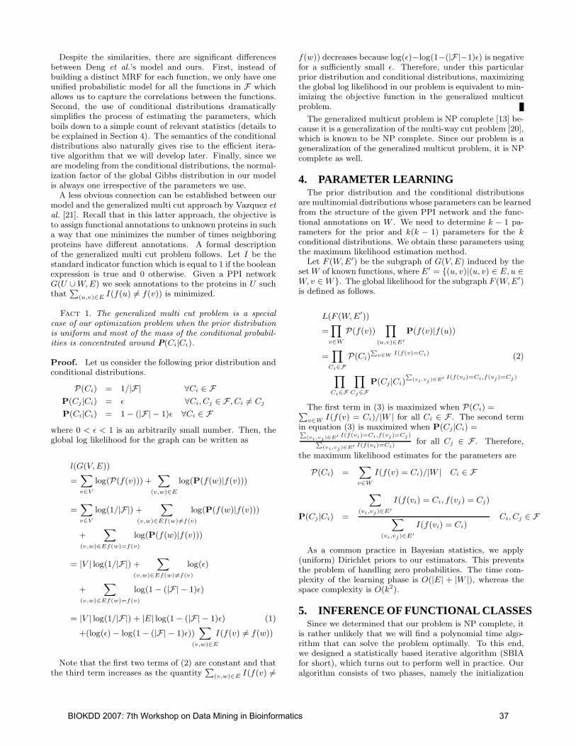
Despite the similarities, there are significant differencesbetween Deng et al.’s model and ours. First, instead ofbuilding a distinct MRF for each function, we only have oneunified probabilistic model for all the functions in F whichallows us to capture the correlations between the functions.Second, the use of conditional distributions dramaticallysimplifies the process of estimating the parameters, whichboils down to a simple count of relevant statistics (details tobe explained in Section 4). The semantics of the conditionaldistributions also naturally gives rise to the efficient itera-tive algorithm that we will develop later. Finally, since weare modeling from the conditional distributions, the normal-ization factor of the global Gibbs distribution in our modelis always one irrespective of the parameters we use.

A less obvious connection can be established between ourmodel and the generalized multi cut approach by Vazquez et

al. [21]. Recall that in this latter approach, the objective isto assign functional annotations to unknown proteins in sucha way that one minimizes the number of times neighboringproteins have different annotations. A formal descriptionof the generalized multi cut problem follows. Let I be thestandard indicator function which is equal to 1 if the booleanexpression is true and 0 otherwise. Given a PPI networkG(U ∪W,E) we seek annotations to the proteins in U suchthat

P

(u,v)∈E I(f(u) 6= f(v)) is minimized.

Fact 1. The generalized multi cut problem is a special

case of our optimization problem when the prior distribution

is uniform and most of the mass of the conditional probabil-

ities is concentrated around P(Ci|Ci).

Proof. Let us consider the following prior distribution andconditional distributions.

P(Ci) = 1/|F| ∀Ci ∈ F

P(Cj |Ci) = ǫ ∀Ci, Cj ∈ F , Ci 6= Cj

P(Ci|Ci) = 1 − (|F| − 1)ǫ ∀Ci ∈ F

where 0 < ǫ < 1 is an arbitrarily small number. Then, theglobal log likelihood for the graph can be written as

l(G(V, E))

=X

v∈V

log(P(f(v))) +X

(v,w)∈E

log(P(f(w)|f(v)))

=X

v∈V

log(1/|F|) +X

(v,w)∈Ef(w) 6=f(v)

log(P(f(w)|f(v)))

+X

(v,w)∈Ef(w)=f(v)

log(P(f(w)|f(v)))

= |V | log(1/|F|) +X

(v,w)∈Ef(w) 6=f(v)

log(ǫ)

+X

(v,w)∈Ef(w)=f(v)

log(1 − (|F| − 1)ǫ)

= |V | log(1/|F|) + |E| log(1 − (|F| − 1)ǫ) (1)

+(log(ǫ) − log(1 − (|F| − 1)ǫ))X

(v,w)∈E

I(f(v) 6= f(w))

Note that the first two terms of (2) are constant and thatthe third term increases as the quantity

P

(v,w)∈E I(f(v) 6=

f(w)) decreases because log(ǫ)−log(1−(|F|−1)ǫ) is negativefor a sufficiently small ǫ. Therefore, under this particularprior distribution and conditional distributions, maximizingthe global log likelihood in our problem is equivalent to min-imizing the objective function in the generalized multicutproblem.

The generalized multicut problem is NP complete [13] be-cause it is a generalization of the multi-way cut problem [20],which is known to be NP complete. Since our problem is ageneralization of the generalized multicut problem, it is NPcomplete as well.

4. PARAMETER LEARNINGThe prior distribution and the conditional distributions

are multinomial distributions whose parameters can be learnedfrom the structure of the given PPI network and the func-tional annotations on W . We need to determine k − 1 pa-rameters for the prior and k(k − 1) parameters for the kconditional distributions. We obtain these parameters usingthe maximum likelihood estimation method.

Let F (W,E′) be the subgraph of G(V,E) induced by thesetW of known functions, where E′ = {(u, v)|(u, v) ∈ E, u ∈W, v ∈W}. The global likelihood for the subgraph F (W,E′)is defined as follows.

L(F (W,E′))

=Y

v∈W

P(f(v))Y

(u,v)∈E′

P(f(v)|f(u))

=Y

Ci∈F

P(Ci)P

v∈W I(f(v)=Ci) (2)

Y

Ci∈F

Y

Cj∈F

P(Cj |Ci)P

(vi,vj)∈E′ I(f(vi)=Ci,f(vj)=Cj)

The first term in (3) is maximized when P(Ci) =P

v∈W I(f(v) = Ci)/|W | for all Ci ∈ F . The second termin equation (3) is maximized when P(Cj |Ci) =P

(vi,vj)∈E′ I(f(vi)=Ci,f(vj)=Cj)P

(vi,vj)∈E′ I(f(vi)=Ci)for all Cj ∈ F . Therefore,

the maximum likelihood estimates for the parameters are

P(Ci) =X

v∈W

I(f(v) = Ci)/|W | Ci ∈ F

P(Cj |Ci) =

X

(vi,vj)∈E′

I(f(vi) = Ci, f(vj) = Cj)

X

(vi,vj)∈E′

I(f(vi) = Ci)Ci, Cj ∈ F

As a common practice in Bayesian statistics, we apply(uniform) Dirichlet priors to our estimators. This preventsthe problem of handling zero probabilities. The time com-plexity of the learning phase is O(|E| + |W |), whereas thespace complexity is O(k2).

5. INFERENCE OF FUNCTIONAL CLASSESSince we determined that our problem is NP complete, it

is rather unlikely that we will find a polynomial time algo-rithm that can solve the problem optimally. To this end,we designed a statistically based iterative algorithm (SBIAfor short), which turns out to perform well in practice. Ouralgorithm consists of two phases, namely the initialization


phase and the iterative phase. The initialization phase con-sists of two steps. In the first step, we estimate the param-eters for the prior distribution and the conditional distribu-tions as described in Section 4. In the second step, we assignan initial functional class to each protein in V , as follows.

For each unknown protein v ∈ U , we assign

f0(v) = argmaxCi∈F P(Ci)Y

(v,t)∈E,t∈W

P(f0(t)|Ci).

In other words, we predict the initial function for v to bethe one that maximizes the local likelihood of v (ignoringneighbors with unknown functions). If v ∈ W , then we setf0(v) to be the function corresponding to annotation in theoriginal data.

In the second phase, we iteratively re-evaluate our predic-tions. For clarity of exposition we use superscripts to de-note the iteration number, i.e., fn(v) denotes the predictedfunctional class for v made in the nth iteration. For eachunknown protein v ∈ U , we set

fn(v) = argmaxCi∈F P(Ci)Y

(v,t)∈E

P(fn−1(t)|Ci).

That is, we adjust our prediction for protein v to be thefunction that maximizes the local likelihood with respect tothe functions predicted for its neighbors in the previous step.Again, if v ∈W , then fn(v) = fn−1(v).

We stop the iterative process as soon as the differencebetween the value of the global likelihood in two consecutivesteps drops below a given threshold. The pseudo-code inFigure 1 summarizes the algorithm. The time complexity ofthe algorithm is O(d|E|), where d represents the number ofiterations (usually d ≤ 5 in our experiments).

6. EXPERIMENTAL RESULTSThe dataset used in our experimental studies is the most

well-characterized PPI network available at the time of writ-ing, namely the network for S. cerevisiae, which is composedof 4,959 proteins and 17,511 interactions. The network wasobtained from the DIP database [16]. We also extracted ahigh confidence yeast PPI network, which is a subset of theyeast PPI network in which interactions that are confirmedby only a single experiment have been removed. This latternetwork has 1,735 proteins and 2354 interactions. The func-tional annotations were obtained from the Gene Ontology(GO) hierarchy [1].

We used cross validation to quantitatively evaluate theprediction accuracy of our algorithm and to compare itsperformance with other methods. In each experiment, werandomly removed the functional annotation to a percent-age p of known proteins, where p ranges from 5% to 95%.This new set of “unknown” proteins served as the test set,called hereafter T . We use W \T to denote the set of knownproteins after p% of them have been “un-labelled” and U todenote the set of the remaining unknown proteins. Clearly,the SBIA’s learning phase (i.e., the computation of the priorand the conditional probabilities) is carried out only on theproteins in W \ T . Learning on the original set W wouldconstitute “cheating”.

So far, in our model we assumed that each protein canperform only one function. This is, however, not true forsome proteins. A protein may participate in multiple bio-logical processes and as a result, it will carry out multiple

functions. In the yeast network, 488 proteins out of 3,022are annotated with two or more top level functions. To han-dle this issue, the nodes in W \ T that are associated withmultiple functions are replicated, so that each copy carriesout exactly one of the annotated functions. Each copy hasthe same interaction partners of the original protein.

As said, the goal is to predict a function for each of theproteins in set T∪U , based on the functional classes in W \Tand the topology of the graph. For each protein in T , wedeclare a prediction to be correct if the predicted functionis one of the functions the protein was originally assigned.The prediction accuracy is calculated as the ratio betweenthe number of correct predictions and the total number ofproteins in the set T . Since the prediction accuracy variesslightly every time we randomly select T , we replicate thesame experiments ten times and compute the average accu-racy. We also record the standard deviation, represented bythe error bars in the figures.

We compared the accuracy of our method against thatof functional flow [13] and against that of the naive ap-proach. We chose to compare SBIA against the functionalflow method because papers [2, 13] report that functionalflow outperforms both majority-rule based methods [17, 8]as well as methods based on the generalized multicut [21,10]. As said, a direct comparison between our method andMRF-based methods [4, 5, 11] is not feasible because theselatter approaches predict more than one functional class foreach protein. The naive method simply predicts the func-tion of a protein to be the most probable functional classaccording to the prior, i.e., argmaxCi∈FP(Ci). Clearly, theexpected prediction accuracy of the naive approach is equalto the ratio between the number of proteins annotated withthe most probable function and the total number |W | ofknown proteins.

We carried out two sets of experiments. In the first set,we considered the seventeen top level molecular functionsdefined in GO. In the yeast PPI network, 3,022 proteins outof 4,959 are annotated with one or more top level functions.The most frequent function is “catalytic activity”, which oc-curs 1,514 times. Thus, the expected prediction accuracyfor the naive approach is 0.501 or 50%. In the high confi-dence yeast PPI network 1,325 proteins are annotated. Themost frequent function in this network is again “catalyticactivity”, which is assigned to 568 proteins. The statisticsof the networks constituting the dataset are summarized inTable 1.

Figure 2-left and 3-left summarize the results of the firstset of experiments on the seventeen functional classes inthe top level of the GO hierarchy. The figures show thatSBIA always outperforms functional flow, especially whenp is large. In the yeast network, the prediction accuraciesof the functional flow algorithm even falls below that of thenaive approach when p is greater than 55%. SBIA, how-ever, still retains good prediction accuracy until p becomeshigher than 70%, and then asymptotically converges to thatof the naive approach. Notice that the initialization phaseof SBIA already achieves a good prediction accuracy. Whenp is less than 80%, the iterative phase improves the predic-tion accuracy even more, along with the global likelihoodof the graph. The number of iterations executed is usuallyrather small, less than 5. When p is greater than 80%, theinformation left in the network is highly incomplete, andas expected the performance of our algorithm falls back to


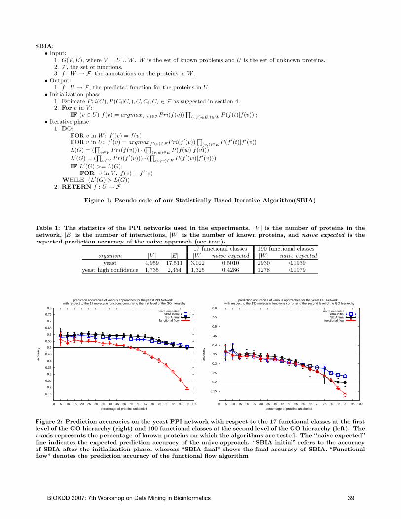
SBIA:• Input:

1. G(V,E), where V = U ∪W . W is the set of known problems and U is the set of unknown proteins.2. F , the set of functions.3. f : W → F , the annotations on the proteins in W .

• Output:1. f : U → F , the predicted function for the proteins in U .

• Initialization phase1. Estimate Pri(C), P (Ci|Cj), C, Ci, Cj ∈ F as suggested in section 4.2. For v in V :

IF (v ∈ U) f(v) = argmaxf(v)∈FPri(f(v))Q

(v,t)∈E,t∈W P (f(t)|f(v)) ;• Iterative phase

1. DO:FOR v in W : f ′(v) = f(v)FOR v in U : f ′(v) = argmaxf ′(v)∈FPri(f

′(v))Q

(v,t)∈E P (f ′(t)|f ′(v))

L(G) = (Q

v∈V Pri(f(v))) · (Q

(v,w)∈E P (f(w)|f(v)))

L′(G) = (Q

v∈V Pri(f′(v))) · (

Q

(v,w)∈E P (f ′(w)|f ′(v)))

IF L′(G) >= L(G):FOR v in V : f(v) = f ′(v)

WHILE (L′(G) > L(G))2. RETERN f : U → F

Figure 1: Pseudo code of our Statistically Based Iterative Algorithm(SBIA)

Table 1: The statistics of the PPI networks used in the experiments. |V | is the number of proteins in thenetwork, |E| is the number of interactions, |W | is the number of known proteins, and naive expected is theexpected prediction accuracy of the naive approach (see text).

17 functional classes 190 functional classesorganism |V | |E| |W | naive expected |W | naive expected

yeast 4,959 17,511 3,022 0.5010 2930 0.1939yeast high confidence 1,735 2,354 1,325 0.4286 1278 0.1979

0.15

0.2

0.25

0.3

0.35

0.4

0.45

0.5

0.55

0.6

0.65

0.7

0.75

0.8

0 5 10 15 20 25 30 35 40 45 50 55 60 65 70 75 80 85 90 95 100

accu

racy

percentage of proteins unlabeled

prediction accuracies of various approaches for the yeast PPI Network with respect to the 17 molecular functions comprising the first level of the GO hierarchy

naive expectedSBIA initialSBIA final

functional flow

0.15

0.2

0.25

0.3

0.35

0.4

0.45

0.5

0.55

0.6

0 5 10 15 20 25 30 35 40 45 50 55 60 65 70 75 80 85 90 95 100

accu

racy


prediction accuracies of various approaches for the yeast PPI Network with respect to the 190 molecular functions comprising the second level of the GO hierarchy


functional flow

Figure 2: Prediction accuracies on the yeast PPI network with respect to the 17 functional classes at the firstlevel of the GO hierarchy (right) and 190 functional classes at the second level of the GO hierarchy (left). Thex-axis represents the percentage of known proteins on which the algorithms are tested. The “naive expected”line indicates the expected prediction accuracy of the naive approach. “SBIA initial” refers to the accuracyof SBIA after the initialization phase, whereas “SBIA final” shows the final accuracy of SBIA. “Functionalflow” denotes the prediction accuracy of the functional flow algorithm


0.15

0.2

0.25

0.3

0.35

0.4

0.45

0.5

0.55

0.6

0.65

0.7

0.75

0.8

0 5 10 15 20 25 30 35 40 45 50 55 60 65 70 75 80 85 90 95 100

accu

racy


prediction accuracies of various approaches for the high confidence yeast PPI Network with respect to the 17 molecular functions comprising the first level of the GO hierarchy


functional flow

0.15

0.2

0.25

0.3

0.35

0.4

0.45

0.5

0.55

0.6

0 5 10 15 20 25 30 35 40 45 50 55 60 65 70 75 80 85 90 95 100

accu

racy


prediction accuracies of various approaches for the high-confidence yeast PPI Network with respect to the 190 molecular functions comprising the second level of the GO hierarchy


functional flow

Figure 3: Prediction accuracy on the yeast high confidence PPI network (see caption of Figure 2 for moredetails). LEFT: 17 functional classes, RIGHT: 190 functional classes.

that of the naive approach. Due to the higher quality of thedata in the yeast high confidence network, the improvementin accuracy of our algorithm and functional flow relative tothe naive approach is almost doubled.

In the second set of experiments, we considered all the 190molecular functions comprising the second level of the GOhierarchy. In the yeast network, 2,930 proteins out of 4,959yeast proteins are annotated with one or more second levelmolecular functions. The most prevalent function is “hydro-lase activity”, which appears 568 times. Hence the expectedprediction accuracy for the naive approach is 0.1939. In thehigh confidence yeast network, 1,278 out of 1,735 proteinsare annotated. The most prevalent function is“protein bind-ing”, which is annotated to 253 proteins. The statistics aresummarized in Table 1.

Figure 2-right and 3-right summarize the second set ofexperimental results. In Figure 3-right, the functional flowalgorithm outperforms SBIA by 2-3% on average. We sus-pect that this is due to the relatively small size of the net-work (containing about 1,300 characterized proteins) underconsideration and the large number of functions (k = 190).Recall that the number of parameters of our model is Θ(k2).In this case, we believe that there is not enough data for theaccurate estimation of the parameters for the prior distri-bution and the conditional distributions. For the yeast PPInetwork, the result is similar to that in the previous set ofexperiments. SBIA still outperforms functional flow, but thedifference between the two approaches is not as strong as inthe previous case.

7. CONCLUSIONSWe developed an efficient algorithm to assign functional

GO terms to uncharacterized proteins on a PPI networkbased solely on the topology of the graph and the functionallabels of known proteins. The statistical model proposedin this paper is a generalization of the GenMultiCut modeland resemble the MRF-based model by Deng et.al. Thesimilarity with the work of Deng et.al. is, however, super-ficial as we discussed in details in the paper. In particular,the structure of our model allows one to obtain easily and

efficiently the maximum likelihood estimation of the under-lying parameters, which is tipically not possible for a generalMRF. Based on our statistical model, we presented efficientlearning and inference algorithms. Our inference algorithmis an iterative algorithm, where each iteration runs in timelinear in the size of the input. According to our experimen-tal results, our algorithm converges very quickly to a localoptimum. More importantly, our method gives consistentlybetter predictions when compared with previous known al-gorithms.

8. REFERENCES[1] Ashburner, M., Ball, C. A., and et al . Gene

ontology: tool for the unification of biology. Nature

Genetics 25 (2000), 25–29.

[2] Chua, H. N., Sung, W.-K., and Wong, L.

Exploiting indirect neighbours and topological weightto predict protein function from protein-proteininteractions. Bioinformatics 22 (2006), 1623 – 1630.

[3] Deng, M., Chen, T., and Sun, F. An integratedprobabilistic model for functional prediction ofproteins. Journal of Computational Biology 11, 2/3(2004), 463–475.

[4] Deng, M., Tu, Z., Sun, F., and Chen, T. Mappinggene ontology to proteins based on protein-proteininteraction data. Bioinformatics 20, 6 (2004), 895–902.

[5] Deng, M., Zhang, K., Mehta, S., Chen, T., and

Sun, F. Prediction of protein function usingprotein-protein interaction data. Journal of

Computational Biology 10, 6 (2003), 947–960.

[6] Formstecher, E., Aresta, S., and et al . Proteininteraction mapping: A drosophila case study.Genome Res. 15, 3 (2005), 376–384.

[7] Giot, L., Bader, J. S., and et al. A proteininteraction map of Drosophila melanogaster. Science

302, 5651 (2003), 1727–1736.

[8] Hishigaki, H., Nakai, K., Ono, T., Tanigami, A.,

and Takagi, T. Assessment of prediction accuracy ofprotein function from protein–protein interactiondata. Yeast 18, 6 (2001), 523–531.


[9] Jaimovich, A., Elidan, G., Margalit, H., and

Friedman, N. Towards an integrated protein-proteininteraction network. In Proceedings of ACM

RECOMB (2005), pp. 14–30.

[10] Karaoz, U., Murali, T. M., Letovsky, S., Zheng,

Y., Ding, C., Cantor, C. R., and Kasif, S.

Whole-genome annotation by using evidenceintegration in functional-linkage networks. Proc Natl

Acad Sci U S A 101, 9 (2004), 2888–2893.

[11] Letovsky, S., and Kasif, S. Predicting proteinfunction from protein/protein interaction data: aprobabilistic approach. Bioinformatics 19, 1 (2003),i197–i204.

[12] Li, S., Armstrong, C., and et al. A map of theinteractome network of the metazoan C. elegans.Science 303 (2004), 540–543.

[13] Nabieva, E., Jim, K., Agarwal, A., Chazelle, B.,

and Singh, M. Whole-proteome prediction of proteinfunction via graph-theoretic analysis of interactionmaps. In Proceedings of ISMB (2005), pp. 302–310.

[14] Rain, J., Selig, L., and et al. The protein-proteininteraction map of Helicobacter pylori. Nature 409

(2001), 211–215.

[15] Rual, J.-F., Venkatesan, K., and et al. Towards aproteome-scale map of the human protein-proteininteraction network. Nature 437 (2005), 1173–1178.

[16] Salwinski, L., Miller, C. S., Smith, A. J.,

Pettit, F. K., Bowie, J. U., and Eisenberg, D.

The database of interacting proteins: 2004 update.Nucleic Acids Research 32 (2004), D449.

[17] Schwikowski, B., Uetz, P., and Fields, S. Anetwork of protein-protein interactions in yeast.Nature Biotechnology 18 (2000), 1257 – 1261.

[18] Srinivasan, B. S., Novak, A. F., Flannick, J. A.,

Batzoglou, S., and McAdams, H. H. Integratedprotein interaction networks for 11 microbes. InProceedings of ACM RECOMB (2006), pp. 1–14.

[19] Uetz, P., Giot, L., and et al. A comprehensiveanalysis of protein-protein interactions inSaccharomyces cerevisiae. Nature 403, 6770 (2000),623–627.

[20] Vazirani, V. V. Approximation algorithms.Springer-Verlag New York, Inc., New York, NY, USA,2001.

[21] Vazquez, A., Flammini, A., Maritan, A., and

Vespignani, A. Global protein function prediction inprotein-protein interaction networks. Nature

Biotechnology 21 (2003), 697.


Profile-feature Based Protein Interaction Extraction from

Full-Text Articles

Shilin Ding1

Minlie Huang1

Hongning Wang1

Xiaoyan Zhu1,∗

ABSTRACT

Various methods have been proposed to extract genetic protein-protein interactions from abstracts. These methods are unable to specify the interactions in which molecules are physically related and fail to explore the abundant evidence all over the articles. In this paper, we present a method of mining physical protein-protein interactions by exploiting profile feature from full-text articles during our participation in the second task of BioCreAtIvE Challenge 2006. This method synthesizes the features from the whole article as the protein pair’s profile to extract the physical interactions, and specifies the SwissProt AC of the molecules involved in the interaction to help biologists make use of the information of the molecules, such as the sequence and cross reference. Compared with the other methods’ performance released in BioCreAtIvE 2006, our method has shown very promising results.

Categories and Subject Descriptors

J.3 [Life and Medical Sciences]: Biology and Genetics; I.5.4 [Pattern Recognition]: Applications – Text Processing

General Terms

Algorithms, Experimentation

Keywords

Protein-Protein Interaction, Text Mining, Information Extraction

1. INTRODUCTION The study of Protein-Protein Interaction (PPI) is one of the most pressing problems. Characterizing protein interaction partners is crucial to understanding not only the functional role of individual proteins but also the organization of entire biological processes. In the past years, the high throughput technologies have generated large amount of information. However, the information is buried in millions of peer-reviewed literatures. Without efficient management, the biological knowledge in the literatures is of little use to the researchers. A lot of knowledge

databases, such as BIND [1], IntAct [11], and MINT [28] have been constructed to this end, but it costs a lot of time and expense to manually review and extract the important information from the literatures. So, automatically mining protein-protein interactions from bioscience literature is crucial and challenging [16].

There are two types of protein interactions: Genetic Interaction which is functional relationship among genes revealed by phenotype of cell, and Physical Interaction which is interaction among molecules. The task we participated in BioCreAtIvE 2006 is focused on mining physical interactions from the text because the genetic interactions are 1) not direct (the interaction may be through signaling cascades), thus, 2) not always trustworthy for biologists [30]. The abstracts with concentrated and limited information from MEDLINE are not capable to provide enough information to accomplish this task, while the full-text articles are more comprehensive to provide the evidence, such as the biological experiment which verifies the existence of the physical interaction. So the major problem here is how to exploit the physical interactions from the evidence

synthesized from the full-text articles.∗

Various methods have been proposed to extract protein-protein interaction. But most of them are focused on abstract and fail to differentiate the physical interaction from the genetic interaction. In this paper, we describe a profile-feature based method to mine physical protein-protein interactions by exploiting abundant features from full-text articles.

The paper is organized as follows: The related works are discussed in Section 2. Section 3 presents the method to recognize the protein molecule names in text and normalize to them to entries in SwissProt. The profile-feature based method to extract the physical interactions from the evidence of the whole article is discussed in Section 4. In Section 5, we show the experiment and evaluation. And we draw our conclusions and discuss the future work in Section 6.

2. RELATED WORK The researches of exploiting the information from the full-text articles are limited due to full texts’ availability and complexity. SGPE [27] used abstracts and full-text articles to extract gene and protein synonyms, and Yu reported that the system performs

∗ Corresponding author: [email protected] Tel: 86-10-62796831 Fax: 86-10-62782266

Permission to make digital or hard copies of all or part of this work for personal or classroom use is granted without fee provided that copies are not made or distributed for profit or commercial advantage and that copies bear this notice and the full citation on the first page. To copy otherwise, or republish, to post on servers or to redistribute to lists, requires prior specific permission and/or a fee. BIOKDD'07, August 12, 2007, San Jose, California, USA. Copyright 2007 ACM 978-1-59593-839-8/07/0008...$5.00.

1State Key Laboratory of Intelligent Technology and Systems (LITS),

Department of Computer Science and Technology, Tsinghua University, Beijing, 100084, China

Email: [email protected], {aihuang,zxy-dcs}@tsinghua.edu.cn, [email protected]


better on full-text articles because the names are more frequently listed in full-text articles. Schuemie [24] in their study of information content in abstracts versus that in full-text articles argued that the information density is higher in abstracts but the information coverage is much greater in full-text articles which indicates that the IE tools will perform better with the various information resources in the full-text articles. And Natarajan [20] used text mining of full-text articles to help generate novel hypothesis for the guide of gene-relation detection experiment and argued that the full-text articles are more comprehensive than the abstracts. So, the previous studies showed that the full-text articles are more effective for the extraction of physically interacted protein pairs.

Various methods and systems [3, 5, 7, 9, 13, 14, 19, 21] have been proposed for protein interaction extraction, but few of them are focused on physical interactions by exploring the evidence synthesized from the full-text articles. One class of these approaches is based on machine learning models. For example, Craven [4] employed a Naïve Bayes Classifier to predict relations from sentences.

Another class of methods for relation extraction is rule-based or pattern-based. The simplest method of this category is to extract relations from co-occurrence of entities in sentences [6, 15]. This method generates high sensitivity but low specificity.

Pattern based methods adopt hand-coded or automated patterns and then use pattern matching techniques to capture relations. Ono [21] manually constructed lexical patterns to match linguistic structures of sentences for extracting protein interactions. Similar hand-coded pattern based systems were also proposed by Rindflesch [23] and Pustejovsky [22]. Such methods contribute high accuracy but low coverage, and moreover, the construction of patterns is time-consuming and requires much domain expertise. Methods which can learn patterns automatically for general relation extraction include SPIES [14], ONBIRES [13, 7], Chiang [3], and Daraselia [5]. Most of them take annotated texts as input, and then learn patterns semi-automatically (starting from some pattern seeds) or automatically. Most of these methods focus on extracting one specific type of relations and can only explore the information confined in one sentence.

The third class of methods analyzes the syntax structures and semantics of the sentences to extract the relations [9]. This method strongly rely on the Natural Language Processing techniques, such as dependence parse trees [18], to get the structure of a particular sentence. This method has promising performance and is able to extract deeper semantic relations from the text. But it is also focused on single sentence and fails to explore the evidence from the whole articles.

In this paper, we describe a method to mine physical protein-protein interactions by exploiting abundant features. A profile-feature based method is adopted to extract the physical interactions from the full-text articles. Every sentence where the candidate molecule pairs co-occur is considered as a piece of evidence. And the profile, which is defined as the representation of the pair’s features all over the article, is constructed based on all of the evidence. Thus, the method is able to exploits the document-level information instead of focusing on the features on sentence level. Here, we use SVM for training and classifying.

Although the information from the whole article is exploited, another difficulty facing physical interaction extraction is how to recognize the molecules in the articles. Since the physical interaction is the interaction between molecules, the identified names should be normalized to entries in a standard database, such as SwissProt. Thus, the biologists can easily get the whole information of the molecules, such as the sequence and taxonomy information, or other abundant cross-reference information.

Previous Named Entity Recognition methods [8, 25, 26, 29] can find out the protein names, but fail to specify what exact molecules these names refer to. The statistical based method is the most prevalent method to recognize named entities in the text. It exploits abundant word form features and context features to train a model [29, 25]. It has promising performance and flexibility but needs a large scale of annotated corpus. The rule based method is fast and highly accurate in a specific domain, but costs a lot of efforts to construct the rules [8]. These two methods are unable to normalize the names to database entries because the lack of reference to protein database. And the dictionary based method has the potential to map the names to the database entries, but the previous ones are only focused on find out the names.

The difficulty is due to extensive ambiguity in names and overlap of names with common English terms [12]. The use of phenotypic description, the conventional abbreviations lead to various synonyms that are difficult to differentiate. Our Named Entity Recognition and Normalization (NER/N) method is a dictionary matching method based on the organism information from the full-text article. We curated the SwissProt database to boost coverage and accuracy of the terms in the database. Then various rules are applied to solve naming convention related problem. The organism information is used to improve the NER/N process in terms of both time and accuracy.

Our contributions in this paper include 1) the novel NER/N method based on the organism information from the full-text article to recognize the protein name and specify the corresponding entry in SwissPort; and 2) the profile-feature based method which exploits the evidence all over the article to extract the physical interaction. In comparison to the average performance of all the submitted runs in BioCreAtIvE 2006, our method shows promising results and is ranked top in the official evaluation.

3. NAMED ENTITY RECOGNITION AND

NORMALIZATION (NER/N) Different from traditional NER, this task requires the protein names be normalized to primary Access Numbers (AC) of SwissProt entries, not just find the original names in the text. The motivation of this task is to help biologists identify the exact molecule of the mentioned protein, so they can use other information of the molecule, such as the sequence and taxonomy, and cross-reference information like protein structure. The major problem here is how to associate the name in the article with the entry in SwissProt.

• First, the inconsistent naming conventions and various usages in text cause a lot of ambiguous terms. For example, TCF, PAL, and PKB may refer to different entities.


• Second, abbreviated terms, such as p53, may cause difficulty for normalization, although domain experts can infer from the context what molecules the author is discussing.

• Third, the same protein name is used to identify different molecules that are from the same or related gene but different organisms. For example, PI3K may refer to different molecules in mouse (P42337), human (P42336), bovine (P32871), produced by the same gene PIK3CA.

• Fourth, the same protein name is used to identify different molecules of different isoforms. For example, PI3K is referred to Q8BTI9 which is the beta isoform of the protein in mouse, and O35904 which is the delta isoform.

As shown in Figure 1, there are mainly four processes in this module: 1) database curation; 2) organism detection; 3) dictionary-matching based name recognition; and 4) normalized names disambiguation. The process is as follows:

1) The SwissProt is curated to incorporate gene names/synonyms and unify the written form;

2) Find all the organisms that are mentioned in the article, mark their positions as an index;

3) The organism list is used to filter out irrelevant SwissProt entries for the matching of current article;

4) The article is processed by the same unification rules and matched by the filtered entries;

5) Disambiguate the multi-mapped names by the organisms in the context

3.1 Database Curation During database curation, two main procedures below are done to improve the quality and coverage of the terms in SwissProt database:

• Curate entry terms in the SwissProt entries. The gene names/synonyms, gene product names/synonyms of the same entry are included. Addition of gene names may

cause ambiguity since a gene may encode several proteins.

• Unify the written form of the entry terms based on rules. The same rules are applied to articles to maintain consistency.

1) Prefixes and suffixes which are not critical for entity identification are removed. For example, prefix c, n and a of PKC, known as Protein Kinase C, which mean conventional, novel and atypical respectively, are removed.

2) Terms with digits or Roman/Greek numbers are transformed into a unified format: Alphabet + white space + digits. This rule implies such normalization: IL-2, IL2, IL 2�IL 2; CNTFR alpha, CNTFR A, CNTFR I�CNTFR 1.

3) Terms not in abbreviated forms are converted to lowercases.

The curation helps to improve the coverage because the official SwissProt names are descriptive and too long to use in articles. And it also helps to solve the nonstandard writing habits due to the rule-based unification.

3.2 Dictionary Matching After curation, there are totally 230,000 entries, and more than 1 million terms. Obviously, it is not feasible for all the terms to be used during dictionary matching with the articles. To improve computation efficiency, we first detect the organisms in an article, and then use the information to rule out irrelevant entries. Our assumption here is that physical interactions described in one article would belong to a limited number of organisms. The organism database used as the controlled vocabulary is NCBI taxonomy [31]. A dictionary matching method is used to detect organisms, and five most frequent organisms are left, marked with their positions in the article. When matching the articles with SwissProt to find the ACs of the protein names mentioned, only the entries belonging to these organisms are used.

In experiment, the matching process saves about three quarters

Figure 1: The Flowchart of NER. First, curate the terms in the SwissProt database; second, find the names and map them to

SwissProt entries; and third, disambiguate the multi-mapped names by zone of control information from the organism contexts.


of the time due to the filtering. The time consumed by matching 740 articles with all entries is 460 minutes on a normal Pentium 4 2.0G processor. Through the filtering process before dictionary matching, the time is reduced to 125 minutes in the same condition.

3.3 Disambiguation One protein name, particularly in abbreviated form, may correspond to multiple SwissProt entries. This is common in cases when the gene products in different organisms are similar (refer to the 3rd and 4th NER problems in Section 2). To solve the disambiguation, the principle of nearest neighbor is used, based on the organism’s zone of control. The presumption here is that every protein name belongs to a particular organism’s context. This context can be determined by the organism’s zone of control (ZOC): beginning from the sentence that mentions the organism till the sentence that mentions another organism. When a multi-mapped name is met, we calculate which organism’s zone the name belongs to based on the nearest neighbor rule, and filter out other maps to SwissProt entries with different organisms.

The disambiguation can’t solve the isoform problems because the name is mapped to different isoforms that belong to the same organism. However the method is efficient because the isoform problems are not prevalent. We will see later in the experiment that this disambiguation method improves the precision greatly with only a little loss in recall.

From the discussion above, it can be inferred that our NER/N method outperforms other methods because: 1) carefully designed curation greatly improves the database’s coverage and eliminates lots of naming inconsistency due to writing habit; 2) the dictionary matching method efficiently maps the name to the SwissProt entries based on the organism information from the full-text article.

4. PROFILE-FEATURE BASED

EXTRACTION Previous methods to extract protein interactions are based on sentence level, thus fail to synthesize the information from the whole articles. However, the topic-level interactions will be discussed at several places across the article, and these places will provide different sources of evidence, such as the experiment support and cross-reference evidence. The basic idea here is to extract interactions by using profile features derived from the whole document. The classifier is trained to make the decision based on the features all over the article. The profile-feature based extraction is more robust than pattern based extraction and other methods focused on the evidence from single sentence.

First, the goal is to extract physical interactions, so the single description as “PTN1 binds to PTN2” does not necessarily indicate the existence of a physical interaction between PTN1 and PTN2. However, if there is other evidence in the document, such as “The bind of PTN1 to PTN2 is determined by two hybrid screen”, then the interaction is more probably to be true. So, different evidence will strengthen the validation of the physical interaction.

Second, the profile-feature based extraction is more robust when NER performance is far from satisfactory. The false positive protein names will falsely pair with other recognized names. But the pairs of the false positive proteins will be less statistically significant all over the document. Their profile features will be more random and less significant. For example, “The Y2H experiment proved the interaction between PTN1 and PTN2, CGA ... …”. The underlined term “CGA” that is the sequence of PTN2 will be recognized as a protein, because CGA is the synonym of Chromogranin A precursor, which is P05059 in SwissProt. This false positive protein will be falsely paired with PTN1 and PTN2. The previous method is hard to filter out the pair even though the pair only appears once in the article. However, the profile-feature based method is able to solve the problem by incorporate the evidence from the whole article.

4.1 Profile Feature Profile features are selected to represent the evidence of a physical interaction. There are 3 types of profile features:

� 168 Unigram/Bi-gram Features 100 of these features are selected by chi-square statistics of

distinctiveness [18], and the rest 68 features are selected from Molecular Interaction (MI) ontology’s [30] definition of Physical Interaction and Detection Method.

� 91 Pattern Features These features are generated in a semi-supervised manner

[7]. These features have a form as “PTN * bind to * PTN”, where PTN indicates a protein entity, and * means any word that can be skipped. The pattern feature is matched against the sentences as a regular expression.

� 2 Position Features One is whether the two proteins co-occur within the title;

the other is whether they co-occur within the abstract.

These features eventually comprise a 261-dimensional feature vector, where each dimension is 1 or 0 indicating the presence or absence of a feature. Examples of these features are shown in Table 1.

Table1: Feature examples

Unigram/Bigram Pattern

aggregation activation of *PTN1 *by *PTN2

crystallography PTN1 bind *PTN2

elongation PTN1 *interact with *PTN2

circular dichroism PTN1 *form complex with *PTN2

4.2 Feature Construction Every protein pair occurred within a sentence is viewed as a candidate. These sentences are considered as evidence. For each pair, profile features are extracted from all the sentences in which the pair appears. The corresponding bit is set as 1 if the feature is found in these sentences, see Figure 2. Through such a representation with abundant features, information from the whole document has been incorporated.


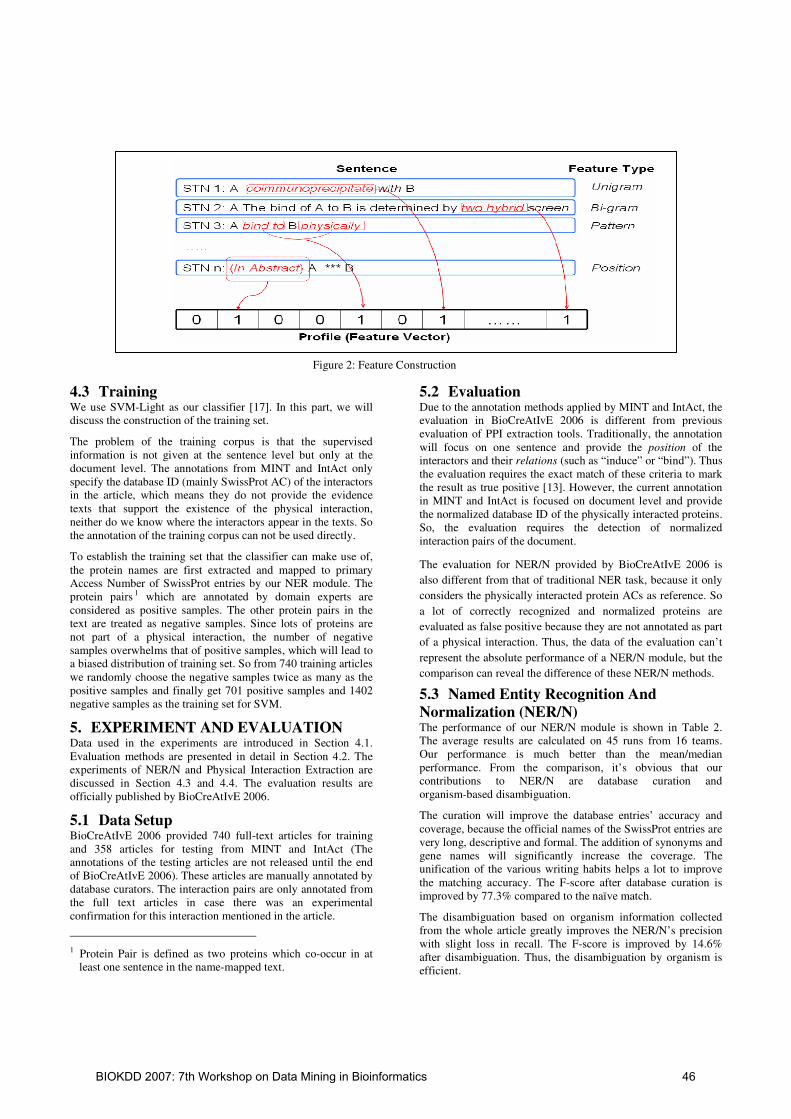
4.3 Training We use SVM-Light as our classifier [17]. In this part, we will discuss the construction of the training set.

The problem of the training corpus is that the supervised information is not given at the sentence level but only at the document level. The annotations from MINT and IntAct only specify the database ID (mainly SwissProt AC) of the interactors in the article, which means they do not provide the evidence texts that support the existence of the physical interaction, neither do we know where the interactors appear in the texts. So the annotation of the training corpus can not be used directly.

To establish the training set that the classifier can make use of, the protein names are first extracted and mapped to primary Access Number of SwissProt entries by our NER module. The protein pairs 1 which are annotated by domain experts are considered as positive samples. The other protein pairs in the text are treated as negative samples. Since lots of proteins are not part of a physical interaction, the number of negative samples overwhelms that of positive samples, which will lead to a biased distribution of training set. So from 740 training articles we randomly choose the negative samples twice as many as the positive samples and finally get 701 positive samples and 1402 negative samples as the training set for SVM.

5. EXPERIMENT AND EVALUATION Data used in the experiments are introduced in Section 4.1. Evaluation methods are presented in detail in Section 4.2. The experiments of NER/N and Physical Interaction Extraction are discussed in Section 4.3 and 4.4. The evaluation results are officially published by BioCreAtIvE 2006.

5.1 Data Setup BioCreAtIvE 2006 provided 740 full-text articles for training and 358 articles for testing from MINT and IntAct (The annotations of the testing articles are not released until the end of BioCreAtIvE 2006). These articles are manually annotated by database curators. The interaction pairs are only annotated from the full text articles in case there was an experimental confirmation for this interaction mentioned in the article.

1 Protein Pair is defined as two proteins which co-occur in at

least one sentence in the name-mapped text.

5.2 Evaluation Due to the annotation methods applied by MINT and IntAct, the evaluation in BioCreAtIvE 2006 is different from previous evaluation of PPI extraction tools. Traditionally, the annotation will focus on one sentence and provide the position of the interactors and their relations (such as “induce” or “bind”). Thus the evaluation requires the exact match of these criteria to mark the result as true positive [13]. However, the current annotation in MINT and IntAct is focused on document level and provide the normalized database ID of the physically interacted proteins. So, the evaluation requires the detection of normalized interaction pairs of the document.

The evaluation for NER/N provided by BioCreAtIvE 2006 is

also different from that of traditional NER task, because it only

considers the physically interacted protein ACs as reference. So

a lot of correctly recognized and normalized proteins are

evaluated as false positive because they are not annotated as part

of a physical interaction. Thus, the data of the evaluation can’t

represent the absolute performance of a NER/N module, but the

comparison can reveal the difference of these NER/N methods.

5.3 Named Entity Recognition And

Normalization (NER/N) The performance of our NER/N module is shown in Table 2. The average results are calculated on 45 runs from 16 teams. Our performance is much better than the mean/median performance. From the comparison, it’s obvious that our contributions to NER/N are database curation and organism-based disambiguation.

The curation will improve the database entries’ accuracy and coverage, because the official names of the SwissProt entries are very long, descriptive and formal. The addition of synonyms and gene names will significantly increase the coverage. The unification of the various writing habits helps a lot to improve the matching accuracy. The F-score after database curation is improved by 77.3% compared to the naïve match.

The disambiguation based on organism information collected from the whole article greatly improves the NER/N’s precision with slight loss in recall. The F-score is improved by 14.6% after disambiguation. Thus, the disambiguation by organism is efficient.

Figure 2: Feature Construction


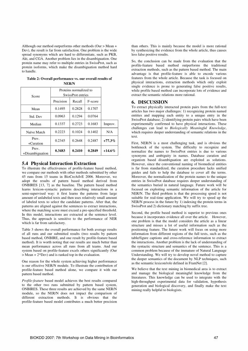
Although our method outperforms other methods (Our > Mean + Dev), the result is far from satisfaction. One problem is the wide spread synonyms which are hard to differentiate, such as PKB, Akt, and CGA. Another problem lies in the disambiguation. One protein name may refer to multiple entries in SwissProt, such as protein isoforms, which make the disambiguation method hard to handle.

Table 2: Overall performance vs. our overall results of

NER/N

Proteins normalized to

SwissProt entries Score

Precision Recall F-score

Mean 0.1495 0.2828 0.1707

Std. Dev 0.0963 0.1294 0.0764

Median 0.1337 0.2723 0.1683 Improv.

Naïve Match 0.2223 0.1024 0.1402 N/A

Prev.

+Curation 0.2345 0.2648 0.2487 +77.3%

Prev.

+Disambiguation 0.3483 0.2410 0.2849 +14.6%

5.4 Physical Interaction Extraction To illustrate the effectiveness of profile-feature based method, we compare our methods with other methods submitted by other 45 runs from 15 teams in BioCreAtIvE 2006. Moreover, we adopt the results of pattern based method derived from ONBIRES [13, 7] as the baseline. The pattern based method learns lexicon-syntactic patterns describing interactions in a semi-supervised way: it first learns the patterns from large amount of unlabeled texts and then uses relatively small amount of labeled texts to select the candidate patterns. After that, the patterns are aligned against the sentences to extract interactions, where the matching score must exceed a pre-specified threshold. In this model, interactions are extracted at the sentence level. Thus, the approach is sensitive to the performance of NER which is far from satisfactory.

Table 3 shows the overall performance for both average results of all runs and our submitted results (two results by pattern based method, ONBIRE, and one result by profile-feature based method). It is worth noting that our results are much better than mean performance across all runs from all teams. And our system based on profile-feature excels others significantly (Our > Mean + 2*Dev) and is ranked top in the evaluation.

One reason for the whole system achieving higher performance is our effective NER/N module. To illustrate the contribution of profile-feature based method alone, we compare it with our pattern based method.

Profile-feature based model achieves the best results compared to the other two runs submitted by pattern based system, ONBIRES. These three results are achieved by the same NER/N module, so the NER/N does not impact the comparison of different extraction methods. It is obvious that the profile-feature based model contributes a much better precision

than others. This is mainly because the model is more rational by synthesizing the evidence from the whole article, thus causes less false positive results.

So, the conclusion can be made from the evaluation that the profile-feature based method outperforms the traditional extraction methods, such as the pattern based method. The main advantage is that profile-feature is able to encode various features from the whole article. Because the task is focused on physical interactions, extraction methods which only exploit single evidence is prone to generating false positive results, while profile based method can incorporate lots of evidence and extract the semantic relations more rational.

6. DISCUSSION To extract physically interacted protein pairs from the full-text articles has two major challenges: 1) recognizing protein named entities and mapping each entity to a unique entry in the SwissProt database; 2) identifying protein pairs which have been experimentally confirmed to have physical interactions. These challenges can lead to Biologically Meaningful Knowledge, which requires deeper understanding of semantic relations in the text.

First, NER/N is a most challenging task, and is obvious the bottleneck of the system. The difficulty to recognize and normalize the names to SwissProt entries is due to various synonyms and ambiguity in names. Database curation and organism based disambiguation are exploited as solutions. However, since the conventional naming of biomedical entities is far from standardized, the curation procedure lacks unified guides and fails to help the database to cover all the terms. Moreover, the normalization of the protein names to the unique entries in SwissProt database requires deeper understanding of the semantics buried in natural language. Future work will be focused on exploiting semantic information of the article for NER/N. The third problem is that the processing speed is not suitable for real-time application. We will try to speed up the NER/N process in the future by 1) indexing the protein terms in SwissProt and 2) dictionary matching by suffix tree.

Second, the profile based method is superior to previous ones because it incorporates evidence all over the article. However, one problem is that the model considers the article as a linear structure and misses a lot of useful information such as the positioning feature. The future work will focus on using more information from different regions of the full texts, such as the table/figure captions and cross-reference information to extract the interactions. Another problem is the lack of understanding of the syntactic structure and semantics of the sentence. This is a common problem because of the immature of Natural Language Understanding. We will try to develop novel method to capture the deeper semantics of the document by NLP techniques, such as the semantic lexicon/role defined in FramNet [2].

We believe that the text mining in biomedical area is to extract and manage the biological meaningful knowledge from the literatures. This knowledge can be used to integrate with the high-throughput experimental data for validation, hypothesis generation and biological discovery, and finally make the text mining really helpful to biologists.


7. ACKNOWLEDGEMENT The work is supported by Chinese Natural Science Foundation under grant No. 60572084 and 60621062, National High Technology Research and Development Program of China (863 Program) under No. 2006AA02Z321, as well as Tsinghua Basic Research Foundation under grant No. 052220205.

8. REFERENCE [1] Bader, G.D., Donaldson, I., Wolting, C., Quellette, B.F.,

Pawson, T. and Hogue, C.W. BIND –The Biomolecular Interaction Network Database. Nucleic Acids Research, 29(1), 2001, pp. 242–245.

[2] Baker, C., Fillmore, C., and Lowe, J. The Berkeley FrameNet project. In Proceedings of the Thirty-Sixth

Annual Meeting of the Association for Computational

Linguistics and Seventeenth International Conference on

Computational Linguistics, pp. 86-90, 1998

[3] Chiang, J.H., and Yu, C.Y. Literature extraction of protein functions using sentence pattern mining. IEEE. Trans. On

Knowledge and Data Enginerring, 17 (8), 2005, pp. 1088-1098.

[4] Craven, M. Learning to extract relations from Medline. AAAI-99 Workshop on Machine Learning for Information

Extraction, 1999.

[5] Daraselia, N., Yuryev, A., Egorov, S., Novichkova, S., Nikitin, A., and Mazo, I. Extracting Human Protein Interactions from MEDLINE Using a Full-Sentence Parser. Bioinformatics, vol. 20(5), 2004, pp. 604-611.

[6] Ding, J., Berleant, D., Nettleton, D., and Wurtele, E. Mining medline: abstracts, sentences, or phrases? In Proceedings of the 7th Pacific Symoisium of Bio-computing, pp. 326–337, 2002

[7] Ding, S.L., Huang, M.L., and Zhu, X.Y. Semi-supervised

Pattern Learning for Extracting Relations from Bioscience Texts. In Proceedings of the 5th Asia-Pacific

Bioinformatics Conference, pp. 307-316, 2007.

[8] Fukuda, K., Tsunoda, T., Tamura, A., and Takagi, T. Toward information extraction: identifying protein names from biological papers. In Proceedings of the 3rd Pacific

Symposium on Biocomputing, pp. 707-718, 1998.

[9] Fundel K., Küffner R., and Zimmer R. RelEx - Relation extraction using dependency parse trees. Bioinformatics, vol. 23, 2007, pp. 365-371

[10] Hanisch, D., Fundel, K., Mevissen, H.T., Zimmer, R., and Fluck, J. ProMiner: Rule-based Protein and Gene Entity Recognition. BMC Bioinformatics 2005, 6 (Suppl 1): S14.

[11] Hermjakob, H., Montecchi-Palazzi, L., Lewington, C., Mudali, S., Kerrien, S., Orchard, S., Vingron, M., Roechert, B., Roepstorff, P., Valencia, A., Margalit, H., Armstrong, J., Bairoch, A., Cesareni, G., Sherman, D., and Apweiler, R. IntAct: an open source molecular interaction database. Nucleic Acids Research, vol. 32, 2004, pp. D452-D455.

[12] Hirschman, L., Yeh1, A., Blaschke, Y., and Valencia, A. Overview of BioCreAtIvE: critical assessment of information extraction for biology. BMC Bioinformatics, 2005, 6 (Suppl): S1

[13] Huang, M.L., Zhu, X.Y., Ding, S.L., Yu, H., and Li, M. ONBIRES: ONtology-based BIological Relation Extraction System. In Proceedings of the Fourth Asia Pacific

Bioinformatics Conference, pp. 327-336, 2006.

[14] Huang, M.L., Zhu, X.Y., Hao, Y., Payan, D.G., Qu, K., and Li, M. Discovering patterns to extract protein-protein interactions from full texts. Bioinformatics, vol. 20, 2004, pp. 3604-3612.

[15] Jelier,R., Jenster, G., Dorssers, L.C., van der Eijk, C.C., van Mulligen, E.M., Mons, B., Kors, J.A. Co-occurrence based meta-analysis of scientific texts: retrieving biological relationships between genes. Bioinformatics, vol. 21, 2005, pp. 2049–2058.

[16] Jensen, L.J., Saric, J., and Bork, P. Literature mining for the biologist: from information retrieval to biological discovery. Nature Reviews Genetics, Vol. 7(2), 2006, pp. 119-129.

Table 3: Physical interaction extraction performance averaged on 45 runs from 16 teams vs. our overall results.

“Whole collection” means all the articles have been considered. “SwissProt only article collection” means articles

containing exclusively interaction pairs which can be normalized to SwissProt entries have been scored.


[17] Joachims, T. Making large-Scale SVM Learning Practical. Advances in Kernel Methods - Support Vector Learning, B. Schölkopf and C. Burges and A. Smola (ed.), MIT-Press, 1999.

[18] Manning, C., and Schütze, H. Foundations of statistical

natural language processing. Cambridge, MA: MIT Press. 1999.

[19] Marcotte, E.M., Xenarios, I., and Eisenberg, D. Mining literature for protein-protein interactions. Bioinformatics, vol. 17, pp. 259-363, 2001

[20] Natarajan, J., Berrar, D., Hack, C., and Dubitzky, W. Knowledge Discovery in Biology Texts: Applications, Evaluation Strategies, and Perspectives. Critical Reviews in

Biotechnology, vol. 25(1-2), 2005, pp. 31-52.

[21] Ono,T., Hishigaki,H., Tanigami,A., and Takagi,T., Automated extraction of information on protein-protein interactions from the biological literature. Bioinformatics, 17(2), 2001, pp. 155-161.

[22] Pustejovsky, J., Castano, J., and Zhang, J. Robust relational parsing over biomedical literature: extracting inhibit relations. In Proceedings of the seventh Pacific Symposium

on Bio-computing, pp 362-373, 2002.

[23] Rindflesch, T., Hunter, L., and Aronson, L. Mining molecular binding terminology from biomedical text. In Proceedings of the AMIA Symposium, Washington, D.C., pp. 127–131, 1999.

[24] Schuemie, M.J., Weeber, M., Schijvenaars, B.J., van Mulligen, E.M., van der Eijk C.C., Jelier, R., Mons, B., and Kors, J.A. Distribution of information in biomedical

abstracts and full-text publications. Bioinformatics, vol. 20(16), 2004, pp. 2597-2604.

[25] Settles, B. Biomedical Named Entity Recognition Using Conditional Random Fields and Rich Feature Sets. In Proceedings of the International Joint Workshop on

Natural Language Processing in Biomedicine and its

Applications (NLPBA), Geneva, Switzerland, pp. 104-107, 2004.

[26] Yoshimasa, T., and Tsujii, J. Boosting Precision and Recall of Dictionary-Based Protein Name Recognition. In Proceedings of the ACL 2003 workshop on Natural

language processing in biomedicine, pp. 41-48, 2003.

[27] Yu, H., Hatzvisaailoulou, V., Friedman, C., Rzhetsky, A., and Wilbur, W.J. Automatic Extraction of Gene and Protein Synonyms from Medline and Journal Articles. In Proceedings of AMIA Symposium, pp. 919-923, 2003

[28] Zanzoni, A., Montecchi-Palazzi, L., Quondam, M., Ausiello, G., Helmer-Citterich, M., Cesareni, G. (2002) MINT: a Molecular INTeraction database. FEBS Letters, vol. 513(1), 2002, pp. 135-140.

[29] Zhou, G.D., Zhang, J., Su, J., Shen, S., and Tan, C.L. Recognizing names in biomedical texts: a machine learning approach. Bioinformatics, Vol. 20 (7), 2004, pp. 1178-1190.

[30] http://www.ebi.ac.uk/ontology-lookup/browse.do?ontName=MI

[31] http://www.ncbi.nlm.nih.gov/entrez/query.fcgi?db=Taxonomy


A Decomposition Approach for DiscoveringNetwork Building Blocks∗

Qiaofeng YangPhysical Biosciences Division

Lawrence Berkeley National LaboratoryBerkeley, CA 94720, USA

[email protected]

Stefano LonardiDepartment of Computer Science & Engineering

University of CaliforniaRiverside, CA 92521, USA

[email protected]

ABSTRACTThe increasing availability of biological networks (protein-protein interaction graphs, metabolic and transcriptionalnetworks, etc.) is offering new opportunities to analyze theirtopological properties and possibly gain new insights in theirdesign principles. Here we concentrate on the problem ofde novo identification of the building modules of networks,which we refer to as network modules.

We propose a novel graph decomposition algorithm basedon the notion of edge betweenness that discovers networkmodules without assuming any a priori knowledge. Weclaim that the knowledge of the distribution of network mod-ules carries more information than the distribution of sub-graphs which is commonly-used in the literature. To demon-strate the effectiveness of the statistics based on networkmodules, we show that our method is capable of clusteringmore accurately networks known to have distinct topologies,and that the number of informative components in our fea-ture vector is significantly higher. We also show that our ap-proach is very robust to structural perturbations (i.e., edgerewiring) to the network. When we apply our algorithm toprotein-protein interaction (PPI) networks, our decompo-sition method identifies highly connected network modulesthat occur significantly more frequently than those foundin the corresponding random networks. Detailed inspectionof the functions of the over-represented network modulesin S. cerevisiae PPI network shows that the proteins in-volved in the modules either belong to the same cellularcomplex or share biological functions with high similarity.A comparative analysis of PPI networks against AS-levelInternet graphs shows that in AS-level networks highly con-nected network modules are less frequent but more tightlyconnected with each other.

Categories and Subject DescriptorsJ.3 [Life and Medical Sciences]: Biology and Genetics;

∗This project was supported in part by NSF CAREER IIS-0447773, and NSF DBI-0321756.

Permission to make digital or hard copies of all or part of this work forpersonal or classroom use is granted without fee provided that copies arenot made or distributed for profit or commercial advantage and that copiesbear this notice and the full citation on the first page. To copy otherwise, torepublish, to post on servers or to redistribute to lists, requires prior specificpermission and/or a fee.BIOKDD ’07 San Jose, California USACopyright 2007 ACM 0-12345-67-8/90/01 ...$5.00.

D.2.8 [Software Engineering]: Design—Methodologies

General TermsGraph theory

1. INTRODUCTIONMany real world systems can be modeled as network graphs,

and their formal analysis can help us understand the un-derlying design principles behind each corresponding sys-tem. For example, identifying highly connected subgraphsin protein-protein interaction graphs can potentially enablelife scientists to discover new protein complexes or specu-late about the functions of unknown proteins [3, 23, 6]. Inaddition, the topological analysis can offer new insights inthe roles of structural elements on the network performance,such as, traffic flow or diffusion of computer viruses over theInternet, epidemic diseases or ideas spreading in social net-works, error and attack tolerance of various communicationnetworks, etc.

In the past few years, a significant research activity hasbeen focused on studying global and local properties of thenetwork graphs (see, e.g., [7, 4, 27]) and significant break-throughs have been achieved. For instance, the concept ofscale-free networks, and the small world phenomenon havechanged the way we model and analyze graphs across manydifferent disciplines, from biological networks, to social net-works all the way to communication networks.

In an attempt to understand the design principles of net-works, the concept of network motif [18] has been recentlyproposed to represent the subgraphs in the network that oc-cur significantly more often than the number of times theyoccur in the corresponding random networks. By using theconcept of network motif, the authors of [18] were able toshow that similar motifs were found in several informationprocessing networks irrespective of their origin. They arguedthat these motifs may define universal classes of networks.The concept of network motif has been widely adopted tostudy local properties of various biological networks. For ex-ample, the network motifs in the transcriptional regulationnetwork of E. coli were studied by Shen-Orr et al. [24]. Theauthors found that three highly significant motifs, namely,the feed-forward loop, the single input module and the dense

overlapping regulons, are the main building blocks of thenetwork. They also discovered that each motif is associatedwith a specific function in determining gene expression. Alarge collection of metabolic pathway networks were ana-lyzed by Koyuturk et al. in [13]. The authors designed


(a) (b) (c)

Figure 1: Illustrating the bias introduced by theoccurrences of hubs (a) on the counts of subgraphs(b) and (c)

an efficient algorithm based on the frequent itemsets algo-rithm [1, 10] to find frequent subgraphs in the metabolicnetworks of over 150 organisms. Wuchty et al. [28] studiedthe conservation of 678 yeast proteins with the correspond-ing ortholog proteins in five higher eukaryotic organisms.The authors discovered that the orthologs are not randomlydistributed in the yeast protein interaction network but arethe building blocks of larger cohesive motifs, which tend tobe evolutionarily conserved. They also observed that largermotifs tend to be conserved as a whole, with each of theircomponents having an ortholog. Yeger-Lotem et al. [31] pro-posed the concept of composite network motifs, which consistof patterns from both transcription-regulation and protein-protein interaction networks that appear significantly moreoften than in random networks. They detected two-protein,three-protein, and four-protein motifs that occur in bothnetworks.

Recently, the concept of network motif has been used toclassify graphs. Milo et al. [17] introduced the concept ofsignificance profile which is computed over the small sub-graphs of the network and is used to cluster different net-works. The profile is a normalized z-score for each sub-graph obtained by comparing the number of occurrences ofthe subgraph to the number of occurrences in correspond-ing random networks. The authors were able to show thatall networks having similar functionality share similar pro-files. Surprisingly a few super-families of unrelated networksalso share very similar significance profiles. Along the sameline, Middendorf et al. [16] proposed a discriminative ap-proach to understand the design of complex networks. Theauthors built a classifier based on alternating decision treeand trained the classifier using raw subgraph counts of 148subgraphs obtained from seven random graph models. Theprotein-protein interaction graph (PPI) of D. melanogaster

was classified as duplication-mutation-complementation net-work [26].

While this paper was under review, a work by Luo et al.

[14] appeared in the scientific literature. The authors presentan agglomerative algorithm to identify biological modules inPPI based on the concept of betweenness and modularity [9,19, 21].

We observe that the majority of the approaches mentionedabove share two common features, namely (1) they are de-signed to operate on directed graphs and (2) they are basedon the exhaustive enumeration of all the subgraphs (up to agiven size) in the network. From here on, we refer to exhaus-tive subgraph enumeration approaches as Subgraph Counting

Network Motif (SCNM) approaches. We observed that usingthe raw subgraph counts as an indicator of over-representa-tion has an inherent shortcoming. This arise from the fact

Input: Graph G, integer k and a list L of all subgraphs gi

of size smaller or equal to kOutput: Number of occurrences of each subgraph gi in L

C ← Connected Components(G)for each connected component Gd ∈ C do

Enqueue(Q, Gd)while Q 6= ∅ do

n, Gc ← 1,Dequeue(Q)if Num Vertices(Gc) ≤ k do

Update Counts(L, Gc)else

while n = 1 do

e← Edge Betweenness(Gc)Remove Edge(Gc, e)C ← Connected Components(Gc)n← Size(C)

for each connected component Gd ∈ C do

Enqueue(Q, Gd)return L

Figure 2: Sketch of the edge betweenness decompo-sition algorithm

that some subgraphs substantially overlap with each other,which in turn creates strong biases in the absolute counts.For example, hubs (nodes with high degree) are quite com-mon in PPI networks [11]. As illustrated in the exampleof Figure 1, if one hub of degree twelve (a) is present inthe network, then we will observe 66 subgraphs of type (b)and 220 subgraphs of type (c). If the network under studyhas several hubs, then type (b) and type (c) subgraphs willbe highly over-represented when compared to random net-works and they will dominate the analysis. However, suchsubgraphs may well be totally irrelevant from a statisticalor biological viewpoint.

Here we address this limitation of SCNM approaches byintroducing a novel graph decomposition method based onthe concept of edge betweenness [9, 19, 21]. Our methoddecomposes the network into a collection of small subgraphs(called network modules), and thereby creates a disjoint par-titioning of the nodes. The fact that a node can belongto only one network module solves the problem of count-ing overlapping subgraphs, and potentially allows us to as-sign putative biological functions to the nodes involved inthe same network module. In order to evaluate objectivelythe effectiveness of our method to extract important fea-tures from the graph, we compare it to SCNM approacheson the problem of graph classification (along the lines of[17]). Results show that our approach is more accuratein distinguishing networks known to have distinct topolo-gies. Our method is also tested for robustness against ran-dom perturbations to the network (i.e., edge rewiring), andour findings suggest low sensitivity to small changes in thegraph. Finally, we report on preliminary results on the anal-ysis of several protein-protein interaction networks (PPI).We show that highly connected network modules are moreover-represented in PPI networks than those found in theirrandom counterparts, and that the proteins involved eitherbelong to the same cellular complex or share highly similarfunctions.

2. AN EDGE BETWEENNESS DECOMPO-SITION ALGORITHM

It is well-known that proteins that are involved in the


��

��

��

��

��

��

��

��

��

��

��

��

��

��

��

��

��

��

��

��

��

��

��

��

��

��

��

��

��

��

��

��

��

��

��

��

��

��

��

��

8 9 107654321

11

21

12 13 14 15

22 23 24 25 26 27 28 29 30 31

16 18 19 2017

Figure 3: Non-isomorphic subgraphs of size ranging from one to five nodes

same cellular process or reside in the same protein complexare expected to have strong interactions with their partners.At the same time, interactions between distinct functionalmodules are expected to be suppressed in order to increasethe overall robustness of the network by localizing effects ofdeleterious perturbations [15]. Biological networks are be-lieved to consist of different modules with distinct functions[11, 22]. Here we are interested in identifying the build-ing blocks of these functional modules without any a priori

biological knowledge.In this study, the detection of the building modules is

based solely on the concept of edge betweenness. Considerthe shortest paths between all pairs of vertices in a graph.The betweenness of an edge [9] is defined as the number ofthese shortest paths running through it1. When two dif-ferent functional modules are loosely connected with eachother, all shortest paths between vertices in those two mod-ules have to traverse the few links between them. By remov-ing those edges, the functional modules are separated fromone another. The effectiveness of the betweenness approachon PPI graph in decomposing the network to find functionalmodules has been recently reported in [6]. In order to findthe basic building modules of the network, we proceed asfollows. First, we compute the edge betweenness of all theedges. Then, we start removing the edges with the high-est betweenness until the largest connected component ofthe graph becomes smaller than or equal to some predefinedthreshold (k). Each time we remove an edge, the between-ness is recomputed from scratch. All the “small” connectedcomponents are then classified and counted. We refer to allthe classified small subgraphs as network modules.

The outline of the algorithm is sketched in Figure 2. Thefunction Edge Betweenness computes and returns the edgewith the largest edge betweenness. Evaluating the between-ness value for all edges of graph G = (V, E) requires O(|V ||E|)time, by running a BFS from each node of the graph. Theiterative removal of all |E| edges leads an overall worst-casetime complexity of O(|V ||E|2) for our approach. Becauseof its computational cost, a distributed implementation ofEdge Betweenness was used [30].

When comparing our approach to Newman and Girvanmethod [19, 21], several major differences emerge. Although

1If multiple shortest paths between a pair of nodes exists,each shortest path contributes an equal fraction to the edge-betweenness of their edges [5].

Table 1: The set of graphs used in the experimentsID name |V | |E|1 H. pylori PPI 702 13592 H. sapiens PPI 1059 13183 C. elegans PPI 2629 39704 S. cerevisiae PPI 4770 151815 D. melanogaster PPI 7057 208156 E.coli. Transcription 418 5197 S. cerevisiae Transcription 688 10788 C. elegans Neuron Connectivity 202 19529 AS1 3522 632410 AS2 4885 927611 AS3 7246 1462912 AS4 10515 2145513 AS5 4686 877214 AS6 9200 2895715 Circuits1 122 18916 Circuits2 252 39917 Circuits3 512 81918 Protein Structure1 95 21319 Protein Structure2 53 12320 Protein Structure3 97 21221 Social1 67 14222 Social2 32 8023 Japanese 2704 799824 English 7381 4420725 French 8325 2384126 Spanish 11586 43065

both algorithms employ betweenness to determine the orderin which edges have to be removed, Newman and Girvan’srelies on a metric that evaluate the quality of the decom-position, called modularity. In their method, the final de-composition is obtained by “cutting” the dendrogram of thedecomposition at the point in which the value of the mod-ularity peaks. In our method, we keep removing edges un-til the graph disconnects; only if the component is smallenough, we stop the process and classify the module in oneof 31 non-isomorphic subgraphs (shown in Figure 3).

Note that in our approach each vertex can only belongto one network module, in contrast to the network motifs

widely used in the literature [18, 24, 28, 31, 16], which arebased on exhaustive subgraph counting (SCNM) approach.To make a distinction between our approach and SCNMapproach, we refer to our method as Graph Decomposition

Network Module (GDNM) approach.


1e-04

0.001

0.01

0.1

1

0 5 10 15 20 25 30

Exhaustive SearchRandom Sampling

Figure 4: Comparing the exhaustive subgraph enu-meration and random sampling on the graph Pro-tein Structure3. The x-axis represents the subgraphindex (according to Figure 3), whereas the y-axisrepresents the subgraph concentration. Subgraphof size 3, 4 and 5 were sampled 100,000 times

3. REPRESENTATION OF GRAPHFEATURES

Since the number of possible subgraphs grows exponen-tially with the number of nodes, in this study we only con-sider the number of occurrences of network modules of sizeup to five nodes (as in papers [20, 28]). As illustrated inFigure 3, there are 31 non-isomorphic subgraphs of sizeup to k = 5. Each subgraph gi is indexed by an integeri = 1, . . . , 31.

When a graph G is processed by the algorithm in Fig-ure 2 where k = 5 and L = {g1, . . . , g31}, a feature vectorof 31 components is returned. Note that the number of oc-currences of subgraphs of size one and two in the SCNMapproaches it is somewhat meaningless, since they corre-spond respectively to the number of nodes and the numberof edges in the graph. As a consequence, the feature vectorfor the exhaustive subgraph counting is 29-dimensional fork = 5. In our approach it is meaningful to keep track of allthose 31 counts because when the network is broken downinto connected components, some of those components mayjust have one or two nodes.

Before we can use these feature vectors to classify graphs,we need to normalize the components to remove the depen-dency on the absolute size of the graph. This will allowus to compare graphs of different sizes. We consider twonormalizations, as explained below.

3.1 Subgraph Proportion NormalizationThe first normalization tries to capture what proportion

of nodes belongs to each subgraph class gi. Given a graphG = (V, E) and the vector [ni] of network module counts,the i-th component of the subgraph proportion vector is de-fined as ni|gi|/|V | where ni is the number of occurrencesfor subgraph class gi. In the following we will use this nor-malization for the feature vectors associated with networkbuilding modules computed by our GDNM decomposition.Note, that since

P31i=1 ni|gi| = |V |, the sum of all the com-

ponents of the subgraph proportion vector is always 1.

3.2 Subgraph Concentration NormalizationThe second (alternative) normalization denotes how fre-

quent is one subgraph class with respect to all the otherclasses with the same number of nodes. Given the vector [ni]of subgraph counts, the i-th component of the subgraph con-

centration [12] vector is defined as ni/P

j:|gj |=|gi|nj , where

ni is the number of occurrences of subgraph gi. It is easyto realize that the sum of all the components of the sub-graph concentration vector is always k. In the following wewill use this normalization for the vector associated withthe exhaustive SCNM approaches, since the subgraph pro-portion vector is not feasible for it. If we used the subgraphconcentration normalization for the GDNM approach, wewould loose the information carried by the network modulesof size one and two (both components will be one).

4. RESULTS AND DISCUSSIONTo test the effectiveness of our GDNM approach, we con-

ducted several experiments and compared the results withthe SCNM method. The first set of experiments is aboutgraph classification, both on simulated data and on real net-works (see Table 1 for a summary of the dataset). Five PPInetworks were obtained from DIP database [29] and the restof the networks are from [2]. We also performed a robustnesstest of our technique and computed the over-representedmodules in PPI networks. Then, we studied the biologi-cal functions associated with the over-represented networkmodules found by our algorithm on the yeast PPI network.

4.1 Graph classification

4.1.1 Estimating the subgraph countsDue to the large size of some of the networks in our

dataset, the exhaustive subgraph enumeration is not alwayspossible. In order to obtain the network motifs based onsubgraph counting, we adopted the sampling algorithm byKashtan et al. [12] to compute the number of occurrencesof each subgraph in the network. For completeness of pre-sentation, we briefly review the sampling procedure for asubgraph of size k. (1) Pick an edge e = (u, v) ∈ E uni-formly at random; (2) Set U = {u, v} (3) Compute the setF of vertices that are adjacent to the vertices in U ; (4) Pickone vertex from F at random and add it to U ; (5) Repeatsteps (3) and (4), until the target number k of vertices isreached.

Figure 4 shows a comparison between the exhaustive sub-graph enumeration and the sampling approach for the “Pro-tein Structure 3” network. The figure shows that the sam-pling algorithm gives good approximations of the subgraphconcentration. We compared the sampling approach to theexhaustive count on many other relatively small graphs andin all cases it was capable of producing good estimates.

4.1.2 Classification of Real NetworksThe real-world networks summarized in Table 1 were pro-

cessed along the same lines as the previous experiment. Itis worth noting that we treated all networks as undirectedgraphs although some of them (i.e., transcription regula-tion networks, social networks and language networks) aredirected. Figure 5 shows the two Pearson correlation coef-ficient matrices for the 26 networks for our decompositionalgorithm (left) and the subgraph counting approach (right).


5 10 15 20 25

5

10

15

20

25

−0.8

−0.6

−0.4

−0.2

0

0.2

0.4

0.6

0.8

5 10 15 20 25

5

10

15

20

25

−0.8

−0.6

−0.4

−0.2

0

0.2

0.4

0.6

0.8

Figure 5: Pearson correlation coefficient matrix on the 26 real networks in Table 1 using decompositionnetwork module approach (LEFT) and subgraph counting network motif approach (RIGHT)

Both pictures use the same scale. An inspection of the rightmatrix (corresponding to SCNM) shows that almost all net-works are significantly correlated with one another. On theother hand, the feature vectors computed with our approach(left) show clearly that there are several distinct families ofnetworks. The first is a big cluster composed of biologi-cal networks (PPI, transcriptional and neural), Internet AS-level networks, and languages networks, although the neu-ral network does not share significant similarity with somemembers of this family. The second consists of circuit net-works and the third consists of protein structure networks.The two social networks are not strongly correlated probablydue to their small size. Note that circuit, protein structureand social networks are clustered together in the SCNM cor-relation matrix (right).

4.1.3 Principal component analysisIn order to establish an objective measure of the quality

of the features extracted by the two approaches, we per-formed a principal component analysis (PCA) of the covari-ance matrices for both methods and both datasets (randomand real data). The goal of this PCA analysis is to es-tablish the effective dimensionality of the feature vectorsobtained by the two methods. Figure 6 shows the distribu-tion of the eigenvalues of the covariance matrix for random(left) and real networks (right). The value of the eigenvaluesclearly illustrates that our decomposition method extractsmore information from the graph. The analysis shows thatour approach has a larger number of significant indepen-dent components in the feature vectors. For example on therandom dataset, 11 principal components have significanteigenvalues whereas only three are obtained using the sub-graph counting approach. On the real network dataset, ourmethod extracts 21 significant components against 14 of theother approach. The fact that we have more “useful” com-ponents in our feature vectors can explain why our approachcreates sharper and more accurate boundaries between dif-ferent types of graphs.

4.2 RobustnessTo test the sensitivity of the GDNM approach to random

perturbation to the graph, we conducted a few experimentsin which we swapped some of the edges of the network at

random. This process is called rewiring [4], and works asfollow.

Given a graph G(V, E), randomly pick two edges (u, v) ∈E and (x, y) ∈ E. If (u, x) /∈ E and (v, y) /∈ E, add (u, x)and (v, y) to E and delete (u, v) and (x, y) from E. Other-wise, if (u, y) /∈ E and (v, x) /∈ E, add (u, y) and (v, x) toE and delete (u, v) an d(x, y) from E. If both choices arefeasible, then whether we should connect (u, x) and (v, y) or(u, y) and (v, x) is arbitrarily chosen at random.

Figure 7 shows the profile of the vectors computed by ourdecomposition method before and after random perturba-tions up to 10% edge-rewiring on the PPI networks of yeastand fly. The figures indicate that our approach is quite ro-bust to random perturbations.

4.3 Enrichment of Network Modules in PPIWe applied our GDNM algorithm to two large biological

networks, namely, the protein-protein interaction (PPI) net-work for S. cerevisiae (yeast) and the PPI for D. melanogaster

(fly). According to [8] the PPI of drosophila was obtainedby high-throughput yeast two hybrid assays, whereas thesource of the PPI data for yeast is a mix of mass spectrome-try and yeast two hybrid assays. Our objective on PPIs is toidentify network modules which are over-represented whenthey are compared to corresponding random networks, andpossibly determine whether these over-represented modulesare associated with important biological functions. We stud-ied over-represented network modules both analytically andempirically. We performed an analytical analysis based onER random graph model and an empirical analysis basedon scale-free network model. We also report a preliminarycomparative analysis of PPI and AS-level networks.

Consider an Erdos-Renyi (ER) random graph G(V, E),which has |V | = n labeled vertices and each pair of vertices isconnected with probability p. Given G we want to calculatethe expected number of occurrences of subgraphs Hr,l withr vertices and l edges. Let Zr,l be the random variableassociated with the number of subgraphs Hr,l in G. Theexpected number of occurrences of Hr,l can be obtained asfollows

E(Zr,l) =

n

r

!

r(r − 1)/2

l

!

pl(1 − p)(r(r−1)/2)−l.


1e-06

1e-05

1e-04

0.001

0.01

0.1

1

0 2 4 6 8 10 12 14 16 18 20

GDNMSCNM

1e-06

1e-05

1e-04

0.001

0.01

0.1

1

0 5 10 15 20 25

GDNMSCNM

Figure 6: The eigenvalue distribution of the covariance matrix for 20 random networks (LEFT) and 26 realnetworks (RIGHT). The x-axis represents the ranks of the eigenvalues, the y-axis represent the absolutevalue of the eigenvalues

Indeed, there are`

n

r

´

ways of selecting r vertices from nvertices, and the maximum number of edges over r verticesis`

r

2

´

= r(r − 1)/2. The probability of observing l edges

given r vertices is therefore`

r(r−1)/2l

´

pl(1 − p)(r(r−1)/2)−l.The value of E(Zr,l) is not a tight reference point whenused to evaluate the significance of the subgraph countsobtained using our GDNM approach. The reason is thatthe count captured by Zr,l include overlapping and discon-nected subgraphs, whereas our approach only considers non-overlapping and connected subgraphs.

Table 2 lists the observed and expected number of sub-graphs Hr,l in the yeast PPI network. It is obvious fromTable 2 that densely connected subgraphs, such as g28−g31,are significantly over-represented when compared with theER random graph model.

When comparing network module counts with the ex-pected number of subgraphs in the ER random model, an-other fact need to be taken into account. Since our methodremoves edges with high betweenness first, it tends to fa-vor highly connected subgraphs to sparser subgraphs. Thisobservation has to be taken into account in the assessmentof the statistical significance of these findings. In order toeliminate this bias, we also conducted an empirical analysisof the statistical significance, as described next.

To better understand the distribution of the number ofsubgraphs when the underlying random graph model hasthe same degree distribution as the original network, weperformed an empirical study based on scale-free networkmodel. The random networks were generated using the samemethod used to generate the scale-free networks above, butthis time the degree distributions are that of the yeast andfly PPI networks. We made sure that the degree distribu-tions are well preserved between real and random networks(statistics not shown). Our GDNM approach was subse-quently applied on the scale-free random networks.

Figure 8 shows the profile of the subgraph proportionvectors for yeast (left) and fly (right) networks comparedto the subgraph proportion vectors obtained from the ran-dom networks with the same degree distribution (averagedover 10 random networks). The comparison shows that largehighly-connected subgraphs (i.e., those with high subgraph

Table 2: The observed and expected number of sub-graphs with r vertices and l edges.

Network module r l Observed Expectedg3 3 2 214 97629g4 3 3 8 45g5 − g6 4 3 118 1.05 e6g7 − g8 4 4 20 1085g9 4 5 6 0.60g10 4 6 3 1.38 e−4g11 − g13 5 4 137 1.41 e7g14 − g18 5 5 18 23430g19 − g23 5 6 26 27g24 − g27 5 7 18 0.02g28 − g29 5 8 7 1.10 e−5g30 5 9 18 3.38 e−9g31 5 10 29 4.66 e−13

indices) occur significantly more often in PPI networks thanin random networks. This indicates that the occurrences ofdensely connected modules in PPI networks cannot be ex-plained by chance and may imply important biological rolesin the cell. When interpreting these results, we should notforget how the PPI data is collected. For example, since co-immunoprecipitation detects multi-protein complexes, thisin turn can possibly bias the number of occurrences of cliquesor other highly connected modules. An open question is howto correct for this bias, since the technology used in the col-lection of protein interaction data is likely to stay with us,at least in the short term.

It is clear from both analytical and empirical approachesthat densely connected modules are significantly over-repre-sented. In order to gain some insights in the functions ofthese modules in PPI networks we concentrated on moduleg31 (5-clique), which is one of the statistically significantmodules identified in the yeast network. The functionalanalysis of the 29 occurrences of module g31 obtained byour algorithm reveals two classes of modules. In the first wefound cellular protein complexes, such as 26S protease, RNApolymerase II, spliceosome, origin recognition complex, nu-clear pore complex, etc. In the second, we found proteins


1e-04

0.001

0.01

0.1

1

0 5 10 15 20 25 30 35

YeastYeast_rewiring

1e-05

1e-04

0.001

0.01

0.1

1

0 5 10 15 20 25 30 35

FlyFly_rewiring

Figure 7: Testing the robustness of our decomposition approach before and after 10% edge rewiring in S.

cerevisiae (LEFT) and D. melanogaster (RIGHT)

1e-04

0.001

0.01

0.1

1

0 5 10 15 20 25 30 35

YeastYeast_random

1e-04

0.001

0.01

0.1

1

0 5 10 15 20 25 30 35

FlyFly_random

Figure 8: Comparing the occurrences of network modules in S. cerevisiae (LEFT) and D. melanogaster

(RIGHT) against the corresponding random graphs (averaged over 10 random graphs)

that share highly similar functions, of which are involvedin transcription regulation, translation initiation, cell cyclecontrol, cellular transportation, mRNA processing, signaltransduction cascades, etc. The functional categories of the29 occurrences of module g31 are summarized in Table 3. Ex-amples of the proteins involved in some of the modules g31

are given in Table 4. Due to lack of space, we refer the readerto http://www.cs.ucr.edu/~qyang/ for the complete set ofannotations.

We also performed a comparative analysis of the networkmodules in PPI networks against Internet AS-level networks.The goal of the analysis was to determine whether the over-represented modules in PPI are more or less interconnectedthan in the AS-level graphs AS4 and AS5. Both PPI andAS-level graphs have a skewed degree distribution. The“richclub connectivity”[32] analysis on the AS4 and AS5 reportedone 10-clique among the vertices with the highest degree(data not shown), which is referred as the core of the Inter-net. Figure 9 shows that the yeast PPI has significantly moreoccurrences of large network modules (e.g., g25, g26, . . . , g31)than AS4 and AS5. Internet AS-level networks are known

Table 3: Distribution of the 5-cliques based on func-tion annotation in S. cerevisiae PPI network

Function Category Number of 5-cliquesTranscription 7mRNA processing 5Cell cycle 5Cellular transportation 4Metabolism 3Translation 2Cytoskeleton 1

to have highly connected core structure, where the links in-side the core carry higher amount of communication flowthan rest of the links in the network. Therefore, links insidethe core will have higher betweenness and will be removedfirst in the decomposition process. The consequence is thatin AS-level networks the resulting decomposition will lackthese large network modules. In contrast, the highly con-


1e-04

0.001

0.01

0.1

1

0 5 10 15 20 25 30 35

YeastAS4

1e-04

0.001

0.01

0.1

1

0 5 10 15 20 25 30 35

YeastAS5

Figure 9: Comparing the occurrences of network modules between S. cerevisiae PPI network and the InternetAS-level network AS4 (LEFT) and AS5 (RIGHT)

nected large modules in PPI networks tend to be more fre-quent and more loosely connected with each other. Thismay indicate that PPI networks are organized in a decen-tralized manner across multiple functional domains, insidewhich strong connections among proteins may constitute thecore facility for carrying out specific functions.

5. CONCLUSIONSIn this paper we proposed a new graph decomposition ap-

proach that is based on the concept of edge betweenness.The decomposition breaks the network into a set of smallnetwork modules, whose frequency of occurrence is thenmapped to feature vectors and then normalized. The ex-periments show that our decomposition method producesnormalized feature vectors that more clearly define classesof graphs than the ones produced by the subgraph counting(network motif) approach. More specifically, the analysis ofthe eigenvalues of the principal components of the covariancematrices shows that our approach extracts a larger numberof independent informative features.

Our method turns out to be quite robust to edge rewiringand therefore not over-sensitive to small perturbations to thegraph. The analysis of the PPI networks of yeast and fly hasidentified several over-represented modules when comparedto random networks with the same degree distribution, andAS-level Internet graphs. A preliminary investigation on theproteins associated with the cliques found by our decompo-sition algorithm on the yeast PPI network shows that theproteins involved either belong to the same complex or sharesimilar biological function.

We conclude by addressing some of the limitations of ourmethod that could point to future research direction. Themain advantage of a decomposition approach is that onenode belongs to only one module, thereby solving the prob-lem of over-counting overlapping subgraphs. However, onPPI graphs this is also a disadvantage because one proteincan belong to only one network module, but it is well-knownthat proteins can be involved in multiple pathways or com-plexes. In order to capture the notion of “soft-partitioning”on graphs, a radically novel approach might be needed. Forexample, recent approaches [33] use the notion of informa-

tion bottleneck [25] to obtain soft partitions of graphs. Also,although our method is not as expensive as the process ofcounting exhaustively all the subgraphs in a large network,it is still quite computationally intensive. The high com-putational cost of our method and other graph clusteringmethods remains an hindrance to their application on largenetworks.

6. REFERENCES[1] R. Agrawal and R. Srikant. Fast algorithms for mining

association rules. Proc. 20th Int. Conf. Very Large

Data Bases, pages 487–499, 1994.

[2] U. Alon. http://www.weizmann.ac.il/mcb/UriAlon/.

[3] G. D. Bader and C. W. V. Hogue. An automatedmethod for finding molecular complexes in largeprotein interaction networks. BMC Bioinformatics, 4,2003.

[4] A.-L. Barabasi and R. Albert. Emergence of scaling inrandom networks. Science, 286:509–512, 2002.

[5] U. Brandes. A faster algorithm for betweennesscentrality. Journal of Mathematical Sociology,25:163–177, 2001.

[6] R. Dunn, F. Dudbridge, and C. M. Sanderson. Theuse of edge-betweenness clustering to investigatebiological function in protein interaction networks.BMC Bioinformatics, 6(39), 2005.

[7] M. Faloutsos, P. Faloutsos, and C. Faloutsos. Onpower-law relationships of the internet topology. ACM

SIGCOMM’99 Comput. Commun. Rev., 29:251–263,1999.

[8] L. Giot, J. S. Bader, C. Brouwer, and et al. A proteininteraction map of Drosophila melanogaster. Science,302:1727–1736, 2003.

[9] M. Girvan and M. E. J. Newman. Communitystructure in social and biological networks. PNAS,99(12):7821–7826, 2002.

[10] K. Gouda and M. J. Zaki. Efficiently mining maximalfrequent itemsets. Proceedings of the 2001 IEEE

International Conference on Data Mining, pages163–170, 2001.


Table 4: Annotations of some 5-cliques in S. cerevisiae PPI network (all the annotation can be found athttp://www.cs.ucr.edu/~qyang/)

DIP ID Description of the proteins Molecular function1 DIP:1112N Pre-mRNA splicing factor PRP19 Involved in pre-mRNA splicing and cell cycle control

DIP:1682N Pre-mRNA splicing factor ISY1DIP:1681N Pre-mRNA splicing factor SYF1DIP:1684N Pre-mRNA splicing factor SYF2DIP:1685N Pre-mRNA splicing factor CLF1

2 DIP:2285N Origin recognition complex subunit 2 Components of origin recognition complex (ORC)DIP:2286N Origin recognition complex subunit 3DIP:2287N Origin recognition complex subunit 4DIP:2288N Origin recognition complex subunit 5DIP:2289N Origin recognition complex subunit 6

3 DIP:1704N Eukaryotic translation initiation factor 3RNA-binding subunit

Eukaryotic translation initiation factors which bind to the40S ribosome and promote the binding of methionyl-tRNAiand mRNA

DIP:2519N Eukaryotic translation initiation factor 390 kDa subunit

DIP:5870N Eukaryotic translation initiation factor 3110 kDa subunit

DIP:4532N Possible eukaryotic translation initiationfactor 3 30 kDa subunit

DIP:2303N Eukaryotic translation initiation factor 54 DIP:1587N 26S protease regulatory subunit 6B ho-

mologComponents of 26S protease complex

DIP:2883N 26S protease regulatory subunit 7 ho-molog

DIP:2100N 26S proteasome regulatory subunitRPN10

DIP:5261N 26S proteasome regulatory subunit RPN9DIP:2808N Proteasome component C11

5 DIP:866N Nucleoporin NUP57 Components of the nuclear pore complex (NPC)DIP:709N Nucleoporin NUP49/NSP49DIP:2074N Nucleoporin NUP145 precursorDIP:2430N Nucleoporin NUP84DIP:2721N Nucleoporin NUP120

[11] J.-D. J. Han, N. Bertin, T. Hao, D. S. Goldberg, G. F.Berriz, L. V. Zhang, D. Dupuy, A. J. M. Walhout,M. E. Cusick, F. P. Roth, and M. Vidal. Evidence fordynamically organized modularity in the yeastprotein-protein interaction network. Nature,430:88–93, 2004.

[12] N. Kashtan, S. Itzkovitz, R. Milo, and U. Alon.Efficient sampling algorithm for estimating subgraphconcentrations and detecting network motifs.Bioinformatics, 20:1746–1758, 2004.

[13] M. Koyuturk, A. Grama, and W. Szpankowski. Anefficient algorithm for detecting frequent subgraphs inbiological networks. Bioinformatics, 20:i200–i207,2004.

[14] F. Luo, Y. Yang, C.-F. Chen, R. Chang, J. Zhou, ,and R. H. Scheuermann. Modular organization ofprotein interaction networks. Bioinformatics,23:207–214, 2007.

[15] S. Maslov and K. Sneppen. Specificity and stability intopology of protein networks. Science, 296:910–913,2002.

[16] M. Middendorf, E. Ziv, and C. H. Wiggins. Inferringnetwork mechanisms: The drosophila melanogasterprotein interaction network. PNAS, 102:3192–3197,2005.

[17] R. Milo, S. Itzkovitz, N. Kashtan, R. Levitt,S. Shen-Orr, I. Ayzenshtat, M. Sheffer, and U. Alon.

Superfamilies of evolved and designed networks.Science, 303:1538–1542, 2004.

[18] R. Milo, S. S. Shen-Orr, S. Itzkovitz, N. Kashtan,D. Chklovskii, and U. Alon. Network motifs: simplebuilding blocks of complex networks. Science,298:824–827, 2002.

[19] M. E. J. Newman and M. Girvan. Finding andevaluating community structure in newtorks. Physical

Review E, 69, 026113, 2004.

[20] N. Przulj, D. G. Corneil, and I. Jurisica. Modelinginteractome: Scale-free or geometric. Bioinformatics,20:3508–3515, 2004.

[21] F. Radicchi, C. Castellano, F. Cecconi, V. Loreto, andD. Parisi. Defining and identifying communities innetworks. PNAS, 101:2658–2663, 2004.

[22] A. W. Rives and T. Galitski. Modular organization ofcellular networks. PNAS, 100(3):1128–1133, 2003.

[23] R. Sharan, T. Ideker, B. P.Kelley, R. Shamir, andR. M.Karp. Identification of protein complexes bycomparative analysis of yeast and bacterial proteininteraction data. RECOMB, pages 282–289, 2004.

[24] S. S. Shen-Orr, R. Milo, S. Mangan, and U. Alon.Network motifs in the transcriptional regulationnetwork of escherichia coli. Nature Genetics, 31:64–68,2002.

[25] N. Tishby, F. Pereira, and W. Bialek. The information


bottleneck method. In Proceedings of the 37-th Annual

Allerton Conference on Communication, Control and

Computing, pages 368–377, 1999.

[26] A. Vazquez, A. Flammini, A. Maritan, andA. Vespignani. Modelling of protein interactionnetworks. ComPlexUs, 1:38–44, 2003.

[27] D. J. Watts and S. H. Strogatz. Collective dynamics of’small-world’ networks. Nature, 393:440–442, 1998.

[28] S. Wuchty, Z. N. Oltvai, and A.-L. Barabasi.Evolutionary conservation of motif constituents in theyeast protein interaction network. Nature Genetics,35:176–179, 2003.

[29] L. Xenarios, L. Salwinski, X. J. Duan, P. Higney,S.-M. Kim, and D. Eisenberg. DIP, the database ofinteracting proteins: a research tool for studyingcellular networks of protein interactions. Nucleic Acids

Research, 30:303–305, 2002.

[30] Q. Yang and S. Lonardi. A parallel algorithm forclustering protein-protein interaction networks.International Journal of Data Mining and

Bioinformatics, 1(3):241–247, 2007.

[31] E. Yeger-Lotem, S. Sattath, N. Kashtan, S. Itzkovitz,R. Milo, R. Y. Pinter, U. Alon, and H. Margalit.Network motifs in integrated cellular networks oftranscription-regulation and protein-proteininteraction. PNAS, 101:5934–5939, 2004.

[32] S. Zhou and R. J. Mondragon. Accurately modelingthe internet topology. Physical Review E Phys. Rev.

E, 70, 2004.

[33] E. Ziv, M. Middendorf, and C. H. Wiggins.Information-theoretic approach to network modularity.Phys. Rev. E, 71, 046117, 2005.


Use of Gene Ontology as a Tool for Assessment of Analytical Algorithms with Real Data Sets: Impact of

Revised Affymetrix CDF Annotation

Megan Kong1, Zhongxue Chen2,3, Yu Qian1, Jennifer Cai1, Jamie Lee1, Eva Rab1, Monnie McGee2, Richard H. Scheuermann1,2

Department of Pathology1 and Department of Clinical Sciences2, University of Texas Southwestern Medical Center,

Dallas, TX and Department of Statistical Sciences3, Southern Methodist University, Dallas, TX Email: [email protected]

ABSTRACT The Gene Ontology™ (GO) of biological process, molecular function and cellular component terms is the predominant source for functional annotation of gene products. An important use of GO-based annotation has been in the interpretation of gene expression microarray results. One of the challenges to gene expression microarray data analysis and interpretation is that cross-hybridization of probes to the related transcripts can contribute to the signal measured. Several recent studies have reported revised microarray probe annotations designed to circumvent this problem by ensuring that the probe annotation matches the current version of the relevant genome sequence and by eliminating probes with sequence similarity to multiple gene, but the impact of these revised annotations remains to be assessed. Here we describe a general approach of using GO annotation co-clustering characteristics to compare the performance of alternative data mining methods, and apply this approach to assess the impact of improved probe annotation on the results of gene expression microarray data interpretation. Using this approach, we found that revised Affymetrix GeneChip® probe annotation gives rise to improved interpretation of microarray gene expression experiments related to the development, function and transformation of human B lymphocytes.

Keywords Bioinformatics, gene ontology, microarray data analysis, microarray annotation.

1. INTRODUCTION An ontology is a formal structured vocabulary that captures the semantic relationships between terms. The standardization of terms and their definitions supports data management and exchange in and between bioinformatics systems. In addition, the formal specification of semantic relationships between the vocabulary terms in the ontological structure supports inference and reasoning that can be used to enhance computational data mining. The Gene Ontology™ (GO) is one of the most successful biomedical ontologies, and includes biological process, molecular function and cellular component terms linked together in a directed acyclic graph with “is_a” and “part_of” relationships [13]. The GO has been used extensively to annotate prokaryotic and eukaryotic gene products based on information described in the scientific literature [2]. An important use of GO-based gene annotation has been to assist in the interpretation of gene expression microarray results [1; 4; 7; 10; 19; 21]. For example, the CLASSIFI algorithm uses GO annotation to classify groups of genes defined by gene cluster analysis using the statistical analysis of GO annotation co-clustering [19]. Gene expression microarrays [12; 24] have fueled a paradigm shift in biomedical research in which reductionistic molecular biology research on individual gene products is augmented by system-level analysis of how the entire transcriptome of a cell population is altered under different normal and pathological conditions. Of the several types of gene expression microarrays that have been developed, the Affymetrix GeneChip® is the most widely used [16]. An Affymetrix GeneChip® can contain from six thousand to more than fifty thousand 25-mer perfect match (PM) oligonucleotide probes with sequences designed to match specific target genes, depending on the organism and platform. Usually the number of PM probes within a probe set is between 11 and 20.

Permission to make digital or hard copies of all or part of this work for personal or classroom use is granted without fee provided that copies are not made or distributed for profit or commercial advantage and that copies bear this notice and the full citation on the first page. To copy otherwise, or republish, to post on servers or to redistribute to lists, requires prior specific permission and/or a fee. BIOKDD'07, August 12, 2007, San Jose, California, USA. Copyright 2007 ACM 978-1-59593-839-8/07/0008...$5.00.

The nature of the microarray technique has brought with it significant challenges in data analysis because of the number of genes being interrogated, the difficulty in controlling and removing the experimental noise, and the need for data normalization to control for inter-experiment variability [11].


Several analytical algorithms, such as MAS5.0 (http://www.affymetrix.com/ products/software/specific/mas.affx), MBEI [20], RMA [16], FARMS [15], and DFW [6] have been developed to deal with these challenges. To assess the performance of these algorithms, a series of data sets were produced in which a group of known transcripts were mixed at known quantities and their levels in the mixture measured using standard microarray methodologies [8; 18]. These so-called “spike-in” data sets provide the ability to assess sensitivity and specificity performance because the true positive and true negative results are known [5; 18; 22]. One of the challenges to gene expression microarray data analysis and interpretation is that cross-hybridization to transcripts related to the target gene of interest can contribute to the fluorescent signal measured. This is especially problematic for the Affymetrix platform because of the relatively short length of each of the oligonucleotide probes. Although the original probe sequences were selected to avoid sequence similarity to related genes, our knowledge of gene and genome sequences has continued to evolve since the current chips were designed. Several recent papers have investigated the quality of Affymetrix GeneChip® probe sets based on current sequence information and found that as much as 30% of the PM probes may be problematic due to potential cross-hybridization and mis-annotation [9; 14; 25]. The Molecular and Behavioral Neuroscience Institute at the University of Michigan (BRAINARRAY, http://brainarray. mbni.med.umich.edu/Brainarray/) has developed new .cdf annotation files for the purposes of annotating Affymetrix chips based on the latest available knowledge of sequences. However, it has been difficult to determine how much this improved annotation will improve the interpretation of Affymetrix GeneChip® using spike-in data sets due to their limited genome coverage. Here we describe a general approach for using GO annotation information to compare the performance of alternative methods for data mining. The approach is based on the postulate that an improvement in any step in the microarray data analysis pipeline should be reflected in improved co-clustering of related genes in real biomedical data sets. This approach was applied to assess the impact of improved Affymetrix GeneChip® probe annotation on the interpretation microarray gene expression experiments related to the development, function and transformation of human B lymphocytes.

2. METHODS

2.1 Data Sets We used several Affymetrix gene expression data sets selected from the GSE2350 series [3] downloaded from the NCBI GEO database (http://www.ncbi.nlm.nih.gov /projects/geo/) in this study. The “Myc” data set consists of 6 microarray chip measurements from cells that conditionally overexpress the c-Myc proto-oncogene (GSM44096 to GSM44101) and 6 measurements from similar cells that do not (GSM44102 to GSM44107). The “Normal B cell Development” data set consists

of 24 measurements of naïve B cell (GSM44133 to GSM44137), centroblast (GSM44143 to GSM44147), centrocyte (GSM44148 to GSM44152), and memory B cell (GSM44138 to GSM44142). The “B cell Response” data set has 18 measurements of Burkitt’s lymphoma B cells stimulated with anti-IgM (GSM44063 to GSM44068) or anti-IgM and anti-CD40L (GSM44069 to GSM44074), and unstimulated controls (GSM44051 to GSM44056). For detailed descriptions of each of the data set, please refer to http://www.ncbi.nlm.nih.gov/projects/geo/.

2.2 Software to Generate the Revised .chp File The revised .cdf annotation file was obtained from the University of Michigan website: http://brainarray.mbni.med.umich.edu/ CustomCDF. We have used the file HS95Av2_HS_3REFSEQ_6 (ACSII version) for generating the revised .chp files. The revised annotations found in this file are based on the use of RefSeq sequence records from the RefSeq database of non-redundant and curated sequences. The original annotation package hgu95av2cdf was obtained from Bioconductor (http://www.bioconductor.org /packages/1.9/AnnotationData.html). For each .cel file, which contains probe-level intensities, .chp file, which contains summarized expression values, were derived following three steps (Figure 1A). This approach to probe set summarization is identical to the default approach supported in the MAS5.0 Affymetrix software. First, the detection p-value was calculated for each probe set using one-sided Wilcoxon signed rank test coded in perl. The default value of τ = 0.015 was used. Then the R value, where R = (PM-MM)/(PM +MM) was calculated for each probe pair. The difference between R and τ was used to calculate the detection p-value for a one-sided Wilcoxon signed rank test. The detection call, present (P), absent (A) or marginal (M), was assigned based on the detection p-value. P-values that were less than 0.04 were assigned a present call, between 0.04 and 0.06 a marginal call, and p-values more than 0.06 received an absent call. The original .chp files and the revised .chp files were generated using both the original .cdf annotation file (HG_U95Av2.cdf) and the revised .cdf annotation file (HS95Av2_HS_3REFSEQ_6.cdf) for each data set, respectively. Second, the summarized expression value for each probe set was calculated in R using MAS5.0 from the Bioconductor affy package (http://www.bioconductor.org/). For the original .chp file calculation, the hgu95av2cdf_1.10.0.zip package was loaded into R, followed by the MAS 5.0 calculation. For the revised .chp file calculation, we used the following R commands to calculate the summarized expression values for the GSM44096 .chp file from the .cel and .cdf files: data<- ReadAffy('GSM44096.CEL') data@cdfName <- "HS95Av2_HS_3REFSEQ_6" s1 = mas5(data) write.exprs(s1, file="revised_mas5_GSM44096.txt") Third, the final .chp files were generated using Perl code by merging the probe set ID, the number of probe pairs in the probe set, the summarized expression value, the detection call, the detection p-value, and the probe set description.


http://www.ncbi.nlm.nih.gov/projects/geo/

http://www.bioconductor.org/

Figure 1. Data processing approaches. A. Generation of revised .chp files using revised .cdf file probe set annotations. B. Filtering, normalization, clustering and cluster classification approaches used to compare effects of revised probe set annotation on Affymetrix microarray data analysis.

2.3 Data Analysis The data analysis approach used is illustrated in Figure 1B. Data filtering, normalization, Significant Analysis of Microarray (SAM) selection of differentially-expressed genes [26] and k-means clustering were performed using TIGR Multiexperiment Viewer (MeV) version 4.0 [23] (http://www.tm4.org/mev.html) as follows. Each data analysis was performed with two categories of samples, with 6 experiment measurements each. For data filtering, only probe sets with at least four present (P) detection calls in either category were selected for further analysis. Data was normalized by columns; specifically, the signal of each probe set in one measurement was adjusted by the mean and the standard deviation (STD) of the signals for this measurement. The normalized signal value equals (x - mean)/STD, where x is the original summarized expression value. SAM was used for the selection of differentially-expressed genes. Initial SAM analysis was performed using all the default settings. Several FDR cutoffs (1%FDR, 5%FDR, or 10%FDR) were used. The combined list of positive and negative differentially-expressed genes from SAM was used to perform k-means clustering analysis. Euclidean distance metric was used in k-means clustering; different numbers of cluster (7, 9, 16, or 20) were used for data set analysis.

The list of all the clusters was saved and formatted to conform to the web-based implementation of CLASSIFI found at: http://pathcuric1.swmed.edu/pathdb/classifi.html. The input format for CLASSIFI is a tab-delimited text file that contains probe set ID (e.g., 13635_at for original annotation, NM_000025_NCBI_refseq for revised annotation), probe set description, and cluster ID. One of the CLASSIFI output files, classifi_topfile, displays the GO term that has the lowest co-clustering p-value for each cluster (see Table 1). Another output file of CLASSIFI, classifi_outputfile, lists all the GO terms in all the clusters with their co-clustering p-values.

2.4 P-value Distribution Assessment The p-values of the co-clustering of GO terms were compared between the CLASSIFI results using the original .cdf annotation and the revised .cdf annotation. To compare the lowest GO term p-values for the clusters obtained, we calculated the mean, the median and the range of the log10 transformed the p-values. To compare the whole distribution of all of the co-clustering GO term p-values for all of the clusters, the Wilcoxon rank sum test was utilized to test whether or not there is a statistically significant difference in the distributions. Briefly, for original p-value list1 of size n1 and revised p-value list2 of size n2, p-values from list1

.cel File

Detection P-value

One-Sided Wilcoxon’s Signed Rank Test

MAS5Probe Set Intensity

Revised .chp File .cel File

Revised .cdf File

perl

Bioconductor R

A

Revised .chp file filter absent genes data normalization SAM significant genes

cluster analysis CLASSIFI analysis

B

Revised .cdf File

Compare GO term P-values from CLASSIFI output

Original .chp file filter absent genes data normalization SAM significant genes

cluster analysis CLASSIFI analysis


http://www.tm4.org/mev.html

http://pathcuric1.swmed.edu/pathdb/classifi.html

Cluster ID GO ID GO Term GO Type g f c n P Value

O1 GO:0006365 35S primary transcript processing BP 1659 4 62 2 7.86E-03

O2 GO:0005575 cellular component CC 1659 1425 191 178 7.26E-04

O3 GO:0016763 transferase activity, transferring pentosyl groups MF 1659 6 22 2 2.44E-03

O4 GO:0006397 mRNA processing BP 1659 73 130 13 3.35E-03 O5 GO:0006796 phosphate metabolism BP 1659 124 68 13 1.09E-03

O6 GO:0016879 ligase activity, forming carbon-nitrogen bonds MF 1659 27 81 6 1.46E-03

O7 GO:0003774 motor activity MF 1659 16 76 5 5.20E-04

O8 GO:0016814 hydrolase activity, acting on carbon-nitrogen (but not peptide) bonds, in

cyclic amidines MF 1659 4 73 3 3.17E-04

O9 GO:0000165 MAPKKK cascade BP 1659 17 116 8 6.44E-06 O10 GO:0030333 antigen processing BP 1659 8 72 4 2.00E-04 O11 GO:0005643 nuclear pore MF 1659 14 231 9 1.81E-05 O12 GO:0031301 integral to organelle membrane CC 1659 8 52 3 1.46E-03 O13 GO:0051082 unfolded protein binding MF 1659 47 39 6 6.00E-04 O14 GO:0019933 cAMP-mediated signaling BP 1659 3 27 2 7.58E-04 O15 GO:0004871 signal transducer activity MF 1659 186 47 13 1.30E-03

O16 GO:0042625 ATPase activity, coupled to transmembrane movement of ions MF 1659 12 44 4 1.83E-04

O17 GO:0003676 nucleic acid binding MF 1659 396 20 14 1.47E-05 O18 GO:0007165 signal transduction BP 1659 289 109 38 4.18E-06 O19 GO:0044237 cellular metabolism BP 1659 899 31 28 1.49E-05 O20 GO:0001568 blood vessel development BP 1659 7 168 5 1.79E-04

R1 GO:0006968 cellular defense response BP 1497 9 16 4 1.07E-06 R2 GO:0005625 soluble fraction CC 1497 25 56 8 1.53E-06 R3 GO:0000062 acyl-CoA binding MF 1497 4 37 3 5.47E-05

R4 GO:0008624 induction of apoptosis by extracellular signals BP 1497 9 36 4 3.27E-05

R5 GO:0008204 ergosterol metabolism BP 1497 3 90 3 2.11E-04 R6 GO:0005635 nuclear envelope CC 1497 26 194 12 2.99E-05 R7 GO:0005663 DNA replication factor C complex CC 1497 4 104 4 2.21E-05 R8 GO:0005537 mannose binding MF 1497 4 61 4 2.50E-06 R9 GO:0000119 mediator complex CC 1497 6 51 4 1.71E-05

R10 GO:0004556 alpha-amylase activity MF 1497 6 57 6 2.34E-09 R11 GO:0006809 nitric oxide biosynthesis BP 1497 4 85 4 9.72E-06 R12 GO:0030529 ribonucleoprotein complex CC 1497 83 32 12 3.49E-08 R13 GO:0019992 diacylglycerol binding MF 1497 18 82 12 4.65E-12

R14 GO:0016755 transferase activity, transferring amino-acyl groups MF 1497 7 69 7 3.27E-10

R15 GO:0019722 calcium-mediated signaling BP 1497 5 54 5 5.08E-08

R16 GO:0009066 aspartate family amino acid metabolism BP 1497 2 58 2 1.48E-03

R17 GO:0015980 energy derivation by oxidation of organic compounds BP 1497 31 44 6 1.93E-04

R18 GO:0004883 glucocorticoid receptor activity MF 1497 7 69 7 3.27E-10 R19 GO:0005794 Golgi apparatus CC 1497 50 88 16 5.11E-09

R20 GO:0000079 regulation of cyclin dependent protein kinase activity BP 1497 5 214 5 5.73E-05

___________________________________________________________________________________________________ Table 1. Comparison of data analysis results from the original and revised annotation files. The "Myc" data set (see Methods) was used in this analysis. Cluster IDs started with letter “O” or “R” represents the clusters obtained from the original or the revised annotation file respectively. In GO type, “BP”, “MF”, or “CC” stands for “biological process”, “molecular function”, or “cellular component” respectively. g, number of probes in data set; f, number of probes with a given ontology in data set; c, number of probes in the gene cluster; n, number of probes with a given ontology (Lee at al., 2006). The GO terms with the lowest p-value in each cluster are displayed.


and list2 were combined and sorted in ascending order. Ranks were assigned to each of the p-value with the smallest p-value getting the rank of 1. The lists of p-values were then separated again and the rank sums were calculated for list1 (sum1) and list2 (sum2). Then, the z-score was calculated based on the approximation: Average: m= n1*(n1+n2+1)/2 Standard Deviation: d=square root (n1*n2*(n1+n2+1)/12) Z score: z= (sum1-m)/d Lastly, the p-value for the distributional comparison was obtained in R using Z-score as input for the function pnorm().

3. RESULTS

Several groups have examined the quality of Affymetrix probe set gene annotation using updated gene/genome sequence information and have found that a substantial number of probes sets are affected [9; 14]. In theory, revisions to the gene annotation of Affymetrix probe sets based on updated genome sequence information would be expected to improve the interpretation of gene expression microarray data. Unfortunately, it has been difficult to assess the impact of revisions to probe set annotation using classical approaches based on the processing of artificial spike-in data sets because a relatively small number of spiked-in transcripts have been used in these data sets and their selection is highly biased toward well-characterized genes. We hypothesized that the co-clustering of genes involved in related biological processes using gene expression microarray data sets from real biological samples could be used to address this limitation, based on the postulate that any improvements made in the pre-processing of gene expression data should result in better co-clustering of related genes. To test the hypothesis that improvements in annotation translate into improvements in interpretation, we compared the extent of co-clustering of related genes using a series of publicly-available Affymetrix gene expression microarray data sets related to human B lymphocyte development and function - GSE2350 [3]. Initially, a microarray data set generated to assess the impact of c-myc overexpression on gene expression patterns in Burkitt’s lymphoma cell lines was evaluated. Details of the data pre-processing procedure employed are described in the Methods section. Briefly (Figure 1), .chp files containing summarized probe set expression values were generated using Affymetrix’s original .cdf annotation files provided in Bioconductor (http://www.bioconductor.org/packages/1.9/AnnotationData.html) (original .chp files) and revised .cdf annotation files developed by the University of Michigan group (http://brainarray.mbni.med.umich.edu/CustomCDF) based on updated probe sequence analysis (revised .chp files). The original and revised .chp files were then processed to remove genes that appeared not to be expressed in the samples used (absent calls), to normalize the summarized expression values to give similar distributions, to select genes that are differentially expressed in the data set using the SAM algorithm [26], to group genes together based on their expression patterns using k-means clustering, and to examine the co-clustering of related genes using the CLASSIFI algorithm [19].

Table 1 lists the GO terms showing the most significant co-clustering characteristics for each of the gene clusters using the original .chp files (Clusters #O1 - #O20) and the revised .chp files (Clusters #R1 - #R20) for the Myc data set. As an example, Cluster #O10 contained a total of 72 probe sets (c) with similar expression characteristics. Four of these probe sets recognized genes that were annotated with the GO term “antigen processing” (n). In this data set, 1659 total probe sets were found to be differentially expressed (g), and 8 of these differentially-expressed genes were annotated with the GO term “antigen processing” (f). Based on the hypergeometric distribution, the probability that 4 of the 8 “antigen processing” genes would co-cluster in a gene cluster of size 72 given that there were 1659 genes evaluated in the data set is 2.00E-04. Out of all of the GO terms that were annotated to genes found in Cluster #O10, the GO term “antigen processing” showed the most significant co-clustering (i.e. lowest p-value, the least likely to have co-clustered based on chance alone). It is difficult to directly compare the co-clustering results derived using the two annotation files based on cluster membership because the numbers and identities of genes that pass the filtering and normalization pre-processing steps differ. However, the extent of co-clustering of related genes can be estimated by assessing the lowest GO term p-values for the clusters obtained. For the Myc data set, using the original .cdf annotation, the mean and median of the log10-transformed lowest p-values for the 20 gene clusters were -3.56 and -3.25, respectively, whereas the mean and median of the log10-transformed lowest p-values using the revised .cdf annotation were -6.08 and -5.31, respectively. In addition, 10 clusters contained all representative genes for a particular gene ontology term from the entire data set when analysis was performed using the revised .cdf annotation (e.g. all 7 glucocorticoid receptor activity genes were found in gene cluster #R18). Whereas no such case of complete co-clustering was found when analysis was performed using the original .cdf annotation file. These data suggest that the use of the revised .cdf annotation leads to more significant co-clustering of related genes in this data set.

FDR cdf Mean Median Range Original -3.56 -3.25 -2.10 to -5.38

1% Revised -6.08 -5.31 -2.84 to -11.1 Original -3.50 -3.58 -2.38 to -5.31

5% Revised -6.98 -6.88 -3.56 to -12.1 Original -4.05 -4.10 -2.12 to -5.39

10% Revised -8.66 -8.80 -3.82 to -13.3

Table 2. Comparison of the co-clustering p-value for most significant GO term using different FDR cut off in SAM analysis. The "Myc" data set (see Methods) was used in this analysis. k-means cluster generated 20 clusters for each FDR cut off. False discovery rate (FDR) cut off of 1%, 5%, or 10% was applied. Values are log10 transformed of the lowest GO term p-value in all the clusters, which represent the mean, the median or the range of the all clusters.


http://www.bioconductor.org/packages/1.9/AnnotationData.html

http://brainarray.mbni.med.umich.edu/CustomCDF

K cdf Mean Median Range

Original -3.23 -3.12 -2.37 to -4.30 7

Revised -6.62 -5.48 -4.55 to -6.79

Original -3.35 -3.12 -2.26 to -5.84 9

Revised -6.00 -5.94 -3.55 to -9.75

Original -3.54 -3.47 -2.48 to -5.75 16

Revised -6.31 -5.57 -3.84 to -11.4

Original -3.56 -3.25 -2.10 to -5.38 20

Revised -6.08 -5.31 -2.84 to -11.1 Table 3. Comparison of the co-clustering p-value for most significant GO term using different number of clusters in k-means analysis. "Revised" annotation or "Original" annotation files were used in analyzing the "Myc" data set (see Methods). 1% FDR was used for SAM analysis. 7, 9, 16 or 20 clusters were generated from k-means clustering. Values are log10 transformed of the lowest GO term p-value in all the clusters, which represent the mean, the median or the range of the all clusters. The use of the revised .cdf annotation also appeared to yield GO terms that reach deeper in the GO hierarchy (i.e. more specific process, function and component terms). For example, using the original .cdf annotation, the most significant GO terms for 6 of the 20 gene clusters were represented more than 100 times (f > 100) in the entire data set indicating a relatively common, high-level annotation term, as compared with zero gene clusters with f > 100 using the revised .cdf annotation (Table 1). The mean value of f dropped from 178 to 15 using the revised .cdf annotation. The assumption is that a greater number of genes would be annotated with GO terms that describe more general functions (e.g. “signal transduction”) than with GO terms that describe more specific functions (e.g. “cell defense response”). Because the numbers and identities of genes that pass the filtering and normalization pre-processing steps differed when using the two different annotation files, it was important to determine if the improved performance of the revised .cdf annotation file was robust to variations in parameters used during data pre-processing steps. Thus, the effects of different false discovery rate (FDR) cutoffs used in the SAM algorithm for the selection of differentially expressed genes were evaluated (Table 2). For all three FDR cutoffs evaluated, the mean, median and range of lowest GO term p-values were all substantially lower when the revised annotation file was used. The effects of different numbers of clusters used in the k-means algorithm were evaluated next (Table 3). Again, for all four values of k evaluated, the mean, median and range of lowest GO term p-values were all substantially lower when the revised annotation file was used. To determine if the improved performance of the revised .cdf annotation might be dependent on the data set used, we evaluated four addition data sets derived from the GSE2350 series (Table 4). For the first three additional data sets, the revised .cdf annotation again out-performed the original .cdf annotation based on the

lowest p-values observed. However, for the fourth additional data set (naïve and memory B cells), the p-value characteristics were much more similar between the two results than was seen with all the other data sets. One possible explanation for this is that the cells used for comparison in this last data set are likely to be much more similar to each other than the cells used in the other data sets. Both naïve and memory B cells are relatively quiescent, and probably only differ from each other by a small subset of genes that change during the relatively small number of differentiation steps between these two cell types. Indeed, the number of differentially expressed genes selected in this data set was much smaller than in the other data sets (611 compared to 1497 from the Myc data set). In the other data sets, many of the comparisons relate to the differences between resting and activated cells of various types, which might be expected to show much larger differences in gene expression patterns. The previous analyses focused on using the GO terms with the single lowest p-values in each gene cluster for comparison. In order to obtain a more complete picture of related gene co-clustering, the entire distribution of p-values for all GO terms in all gene clusters using the two .cdf annotations was compared

Table 4. Comparison of lowest GO term p-values with different microarray data sets. Values are log10 transformed of the lowest GO term p-value in all the clusters, which represent the mean, the median or the range of the all clusters in each data set. The “B-cell anti-IgM” represents data for B cell stimulated with anti-IgM (GSM44063 to GSM44068) and B cell unstimulated controls (GSM44051 to GSM44056) from the “B cell Response” data set. The “B-cell anti-IgM+anti-CD40L” represents data for B cell stimulated with both anti-IgM and anti-CD40L (GSM44069 to GSM44074), and B cell unstimulated controls (GSM44051 to GSM44056) from the “B cell Response” data set. The “Centroblasts&centrocytes” represents data for centroblasts (GSM44143 to GSM 44147) and centrocytes (GSM44148 to GSM44152) from the “Normal B cell Development” data set. The “Naïve and memory B-cell” represents data for naïve B cell (GSM44133 to GSM44137) and memory B cell (GSM44138 to GSM44142) from the “Normal B cell Development” data set. 5%FDR was applied to all the data sets except “Centroblasts &centrocytes”, where 30% FDR was used. Twenty clusters were generated using k-means clustering for all data sets.

Data set cdf Mean Median Range

Original -3.33 -3.39 -1.94 to -6.95B cell anti-IgM

Revised -6.15 -5.33 -3.48 to -11.4

Original -4.93 -4.01 -2.81 to -15.3B cell anti-IgM + anti-CD40 Revised -7.54 -6.83 -3.74 to -15.1

Original -3.25 -2.89 -1.86 to -10.26Centoblasts& centrocytes Revised -5.67 -4.8 -2.21 to -18.46

Original -4.04 -3.17 -1.98 to -18.02Naïve and memory B cells Revised -4.60 -3.96 -1.02 to -7.64

(Figure 2). Throughout the distribution, the number of GO terms with relatively low p-values (p < 0.1) was much higher when using the revised .cdf annotation (Figure 2A). For example, the


number (Figure 2B) and percent (Figure 2C) of GO terms giving p-values below 10-3 was three to four times higher using the revised .cdf annotation. The Wilcoxon rank sum test was used to compare the entire distribution of GO term p-values, in two different data sets at two different FDR cutoffs and two different values for k. The differences in the entire p-value distributions in every case were highly statistically significant (Table 5).

4. DISCUSSION At the present time, there are various tools to analyze microarray data; however, the quality and the validity of these analytical tools need to be assessed fairly. One way to evaluate analytical tools is to analyze spike-in data using these tools and compare the receiver operating characteristic (ROC) curves produced [15; 22]. While this approach is useful, there is some concern that analytical approaches that work well with spike-in data may not work as well with data derived from real, complex biological samples. In addition, ROC analysis is not feasible for real biological data since the true expression values for target mRNA’s are rarely known, and so methods of comparison other than ROC curves are needed. In this study, we examined the possibility of using GO term co-clustering as a comparative tool to assess the impact of using revised annotation on Affymetrix gene expression microarray data analysis. This idea is based on the postulate that genes encoding proteins involved in the same biological process or protein complex will be coordinately expressed; that is, genes that have the same GO annotations are more likely to be in the same gene expression cluster. Thus, better analytical algorithm that gives rise to results that better reflect the underlying biology would be expected to give rise to more significant co-clustering of GO terms. Our analysis comparing the Affymetrix revised and original annotation is the first attempt to use this method to assess the impact the revised annotation has on data analysis. We have analyzed several data sets utilizing different analysis parameters (different FDR, different number of clusters) and calculated the GO term co-clustering probability using the CLASSIFI tool. Our results demonstrate that the p-values for the most significant GO terms in each cluster are significantly lower when using the revised annotation file. In addition, the whole distribution of all the co-clustering p-values for all the GO terms is substantially lower when the revised annotation is used. Thus, using revised annotation indeed produces much more significant co-clustering of related genes. The results showing significant improvement in related gene co-clustering not only suggests that the revised .cdf annotation is better, but also support the general approach of using GO co-clustering as an algorithm evaluation tools with real biological data. In the future, we plan to use the co-clustering method to compare the performance of various preprocessing algorithms on real data sets. Use of gene ontology terms to help interpret systems-level biological data is a great addition to the data analysis arsenal [1; 4; 10; 21; 19]. Although this study has focused on microarray analysis, the same methodology can be applied to other large-scale

1% FDR 5%FDR Data set

k=9 k=16 k=9 k=16

B cell anti-IgM + anti-CD40 1.41E-25 5.18E-27 3.52E-19 4.96E-24

"Myc" data set 5.31E-18 3.01E-32 1.21E-19 2.98E-27

Table 5. Significant differences in the p-value distributions between the results from the original and the revised annotation. To compare the entire distribution of all GO term p-values for all gene clusters using the two annotation files, Wilcoxon rank sum test was employed to test whether or not there is a statistically significant difference in the distributions. 1% or 5%FDR was used in SAM. 9 or 16 clusters were used for k-means cluster. The B-cell stimulated with both anti-IgM and anti-CD40L (GSM44069 to GSM44074) and the B-cell unstimulated controls (GSM44051 to GSM44056) from the “B cell Response” data set and the "Myc" data set (see Methods) were used in this analysis. data sets in which large sets of genes/proteins are analyzed (e.g. protein-protein and genetic interaction networks). Thus, in addition to aiding in the understanding of the functions played by genes and proteins in the cell, the Gene Ontology can also play a role in assisting in the development of improved data mining approaches that reveal underlying functional properties in complex biological systems. 5. ACKNOWLEDGEMENTS The authors wish to acknowledge support for this work from Dr. Milton Packer, Director, Department of Clinical Sciences, University of Texas Southwestern Medical Center and from the National Institutes of Health contracts N01-AI40076, N01-AI40041 to RHS and 1 R15GM079742-01 to MM. 6. REFERENCES [1] Al-Shahrour, F., Díaz-Uriarte R., and Dopazo, J. FatiGO:

a web tool for finding significant associations of Gene Ontology terms with groups of genes. Bioinformatics, 20, 578-580, 2004.

[2] Ashburner, M., Ball, C. A., Blake, J. A., Botstein D., Butler,

H., Cherry, J.M., Davis, A.P., Dolinski, K., Dwight, S.S., Eppig, J.T., Harris, M.A., Hill, D.P., Issel-Tarver, L., Kasarskis, A., Lewis, S., Matese, J.C., Richardson, J.E., Ringwald, M., Rubin, G.M. and Sherlock, G. Gene Ontology: tool for the unification of biology. Nature Genetics, 25, 25 – 29, 2000.

[3] Basso, K., Margolin A.A., Stolovitzky, G., Klein, U., Dalla-

Favera, R., Califano, A. Reverse engineering of regulatory networks in human B cells. Nature Genetics 37, 382-90, 2005.

[4] Bluthgen, N., Brand, .K, Cajavec, B., Swat, M., Herzel, H.

and Beule, D. Biological profiling of gene groups utilizing Gene Ontology. Genome Inform., 16, 106-15, 2005.


A

B C

Figure 2. Comparison of GO term p-value distributions between original and revised Affymetrix probe set annotation. The “Myc” data set (see Methods) was used in this analysis. 1%FDR for SAM analysis and 20 clusters for k-means cluster were applied. A. The distribution of all the p-values for all the GO terms in every cluster. The curve marked with “x” represents the co-clustering p-values using the revised annotation. The dashed line represents the co-clustering p-values using the original annotation. Number of GO terms (B) or the percent of GO terms (C) are plotted against different p-value cut off (P < 10-2, 10-3, 10-4, or 10-5).

1500 10.00

0

500

1000

P<10-2 P<10-4 P<10-5

Num

ber o

f GO

term

s Original Original Revised

0.00

2.00

4.00

6.00

8.00Revised

Perc

ent o

f GO

term

s

P<10-2 P<10-4 P<10-5P<10-3P<10-3


[5] Bolstad, B.M., Irizarry, R.A., Åstrand, M. and Speed, T.P. A comparison of normalization methods for high density oligonucleotide array data based on variance and bias. Bioinformatics, 19, 185-193, 2003.

[6] Chen, Z., McGee, M., Liu, Q., Scheuermann, R. H. A

distribution free summarization method for Affymetrix GeneChip arrays. Bioinformatics, 23, 321-7, 2007.

[7] Conesa, A., Gotz, S., Garcia-Gomez, J.M., Terol, J., Talon,

M. and Robles, M. Blast2GO: a universal tool for annotation, visualization and analysis in functional genomics research. Bioinformatics, 21, 3674-6, 2005.

[8] Cope, L. M., Irizarry, R.A., Jaffee, H.A., Wu, Z., and Speed,

T.P. (2004) A benchmark for Affymetrix GeneChip expression measures. Bioinformatics, 20, 323-331, 2004.

[9] Dai, M., Wang, P., Boyd, A.D., Kostov, G., Athey, B.,

Jones, E.G., Bunney, W.E., Myers, R.M., Speed, T.P., Akil, H., Watson, S.J. and Meng, F. Evolving gene/transcript definitions significantly alter the interpretation of GeneChip data. Nucleic Acids Res., 33, e175, 2005.

[10] Doniger, S.W., Salomonis, N., Dahlquist, K.D., Vranizan,

K., Lawlor, S.C., and Conklin, B.R. MAPPFinder: using Gene Ontology and GenMAPP to create a global gene-expression profile from microarray data. Genome Biol., 4, R7, 2003.

[11] Draghici, S., Khatri, P., Eklund A.C. and Zoltan S.

Reliability and reproducibility issues in DNA microarray measurements. Trends Genet., 22, 101-9, 2006.

[12] Eisen, M.B., Spellman, P.T., Brown, P. O., and Botstein, D.

Cluster analysis and display of genome-wide expression patterns. Proc Natl Acad Sci. U.S.A., 95, 14863–14868. 1998.

[13] The Gene Ontology Consortium. Creating the Gene

Ontology Resource: Design and Implementation. Genome Res., 11, 1425-1433, 2001.

[14] Harbig, J., Sprinkle, R., and Enkemann, S. A. A sequence-

based identification of the genes detected by probesets on the Affymetrix U133 plus 2.0 array. Nucleic Acids Res., 33, e31, 2005.

[15] Hochreiter, S., Clevert, D., and Obermayer, K. A new

summarization method for affymetrix probe level data. Bioinformatics, 22, 943-949, 2006.

[16] Irizarry, R.A., Hobbs, B., Collin, F., Beazer-Barclay, Y.D.,

Antonellis, K.J., Scherf, U. and Speed, T.P. Exploration, normalization, and summaries of high density oligonucleotide array probe level data. Biostatistics 4, 249-264, 2003.

[17] Irizarry, R.A., Bolstad, B.M., Collin, F., Cope, L.M., Hobbs,

B. and Speed, T.P. Summaries of Affymetrix GeneChip probe level data. Nucleic Acids Res., 31, e15, 2003.

[18] Irizarry, R.A., Wu, Z., and Jaffee, H. A. Comparison of

Affymetrix GeneChip expression measures. Bioinformatics, 22, 789-794, 2006.

[19] Lee, J.A., Sinkovits, R.S., Mock, D., Rab, E.L., Cai, J.,

Yang, P., Saunders, B., Hsueh, R.C., Choi, S., Subramaniam, S., Scheuermann, R.H. in collaboration with the Alliance for Cellular Signaling. Components of the antigen processing and presentation pathway revealed by gene expression microarray analysis following B cell antigen receptor (BCR) stimulation. BMC Bioinformatics, 7, 237, 2006.

[20] Li, C., and Wong, W.H. Model-based analysis of

oligonucleotide arrays: Expression index computation and outlier detection. Proc Natl Acad Sci U S A., 98, 31-36, 2001

[21] Martin, D.M., Berriman, M., and Barton, G.J. GOtcha: a

new method for prediction of protein function assessed by the annotation of seven genomes. BMC Bioinformatics, 5, 178, 2004.

[22] McGee., M. and Chen, Z. New spike-in data sets for the

Affymetrix HG-U133a Latin square experiement. COBRA Reprint Series, Article 5, 2006.

[23] Saeed, A. I., Bhagabati, N. K., Braisted, J. C., Liang, W.,

Sharov, V., Howe, E. A., Li, J., Thiagarajan, M., White, J. A. and Quackenbush, J. TM4 Microarray Software Suite, Methods Enzymol., 411, 134-193, 2006.

[24] Schena, M., Shalon, D., Davis, R.W. and Brown, P.O.

Quantitative monitoring of gene expression patterns with a complementary DNA microarray. Science 270, 467-70, 1995.

[25] Shi, L., Reid, L.H., Jones, W.D., Shippy, R., Warrington,

J.A., Baker, SC., Collins, P.J., de Longueville, F., Kawasaki, E.S., Lee, K.Y., Luo, Y. et al. The MicroArray Quality Control (MAQC) project shows inter- and intraplatform reproducibility of gene expression measurements. Nat Biotechnol. 24, 1151-1161, 2006.

[26] Tusher, V.G., Tibshirani, R. and Chu, C. Significance

analysis of microarrays applied to the ionizing radiation response. Proc Natl Acad Sci U S A., 98, 5116–5121, 2001


Clustering of Non-Alignable Protein Sequences Abdellali Kelil

Department of Computer Sciences University of Sherbrooke Sherbrooke, QC, Canada

1 (819) 823 8616

[email protected]

Shengrui Wang Department of Computer Sciences

University of Sherbrooke Sherbrooke, QC, Canada

1 (819) 821 8000 ext 62022

[email protected]

Ryszard Brzezinski Department of Biology

University of Sherbrooke Sherbrooke, QC, Canada

1 (819) 821 8000 ext 61077

[email protected]

ABSTRACT We are interested in the problem of grouping families of non-

alignable protein sequences, such as circular-permutation, multi-

domain and tandem-repeat proteins, into clusters (classes) of

related biological functions. For such sequences, whose numbers

are constantly growing, the commonly used alignment-dependent

approaches fail to yield biologically plausible results. To the best

of our knowledge, no automatic process yet exists to carry out

clustering on these proteins. Biologists often use more complex

manual approaches based on secondary and tertiary structures,

which require considerably more resources and time.

In this paper, we develop a new similarity measure SMS, applied

directly on non-aligned sequences. It allows us to develop a new

and original alignment-free algorithm, named CLUSS, for

clustering protein families based on a spectral decomposition

approach inspired by the latent semantic analysis (LSA) widely

used in information retrieval. CLUSS, utilized jointly with SMS,

is effective on both alignable and non-alignable protein

sequences. To show this, we have extensively tested our algorithm

on different benchmark protein databases and families; we have

also compared its performance with many alignment-dependent

mainstream algorithms. The source code, the application server,

and all experimental results are available at CLUSS web site

http://prospectus.usherbrooke.ca/CLUSS/.

Categories and Subject Descriptors J.3 [Life and Medical Sciences]: Biology and Genetics; I.5.3

[Pattern Recognition]: Clustering

General Terms Algorithms, Measurement, Experimentation

Keywords Clustering, Phylogenetic, Biological Function, Protein Sequences,

Matching, Similarity Measure, Alignable, Non-Alignable

1. INTRODUCTION With the rapid burgeoning of protein sequence data, the number

of proteins for which no experimental data are available greatly

exceeds the number of functionally characterized proteins. To

predict a function for an uncharacterized protein, it is necessary

not only to detect its similarities to proteins of known biochemical

properties (i.e., to assign the unknown protein to a family), but

also to adequately assess the differences in cases where similar

proteins have different functions (i.e., to distinguish among

subfamilies). One solution is to cluster each family into distinct

subfamilies composed of functionally related proteins.

Subfamilies resulting from clustering are easier to analyze

experimentally. A subfamily member that attracts particular

interest need to be compared only with the members of the same

subfamily. A biological function can be attributed with high

confidence to an uncharacterized protein, if a well-characterized

protein within the same cluster is already known. Conversely, a

biological function discovered for a newly characterized protein

can be extended over all members of the same subfamily.

Almost all automatic clustering approaches deal with only aligned

protein sequences, which are performed via alignment algorithms

such as the widely known MUSCLE [8], ClustalW [36], MAFFT

[18] and T-Coffee [26], and many others. These algorithms often

provide information on both conserved and mutated motifs,

making it a good approach for measuring similarities between

protein sequences. However, they have several serious limitations,

including the following:

Dependence on the algorithm used. The results depend heavily

on the algorithm selected and the parameters set by the user for

the alignment algorithm (e.g., gap penalties). As far as easily-

alignable proteins are concerned, almost every existing alignment

algorithm can yield good results. However, for protein sequences

that are difficult to align, each alignment algorithm finds its own

solution. Such variable results create ambiguities and can

complicate the clustering task [25].

Problem of non-alignable sequences. For the case of non-

alignable protein sequences (i.e., not yet definitively aligned),

alignment-based algorithms do not succeed in producing

biologically plausible results. This is due to the nature of the

alignment approaches, which are based on the matching of

subsequences in equivalent positions, while non-alignable

proteins often have similar and conserved domains in non-

equivalent positions [25], such as circular-permutation, multi-

domain and tandem-repeat proteins

Permission to make digital or hard copies of all or part of this work for

personal or classroom use is granted without fee provided that copies are

not made or distributed for profit or commercial advantage and that

copies bear this notice and the full citation on the first page. To copy

otherwise, or republish, to post on servers or to redistribute to lists,

requires prior specific permission and/or a fee.

BIOKDD'07, August 12, 2007, San Jose, California, USA.

Copyright 2007 ACM 978-1-59593-839-8/07/0008...$5.00.


There are other known difficulties that limit the reliability of

alignment, especially for the case of hard-to-align protein

sequences, such as “repeat”, “substitution” and “gap” problems,

which are well discussed by Higgins [15].

The number of protein sequences that are hard-to-align or not

alignable at all is rapidly increasing. These proteins are frequently

related to important biological phenomena, and their classification

is of primary importance for the comprehension of these

phenomena. One example is the group of 33 (/)8-barrel

proteins belonging to the Glycoside Hydrolase (GH) family [35],

which has an important role in the physiology of the alive cell, as

discussed in [5,13]. A large number of these are still

uncharacterized, since to date the process has been carried out

manually with complicated approaches, such as those employed

by Côté et al. [5] and Fukamizo et al. [13] for the characterization

of the 33 (/)8-barrel proteins belonging to the GH [35] family.

Most of the tools currently available are based on the alignment of

protein sequences, making them inappropriate for this kind of

proteins.

Our aim in this paper is to develop a new approach to the

biological interpretation of protein sequences, especially those

which cause problems for alignment-dependent algorithms. Our

work is an attempt to build an algorithm to help biologists

perform analyses of certain kinds of protein sequences, which are

now carried out almost manually. In the rest of the paper, we use

the terms subfamily and cluster interchangeably.

2. RELATED WORK The literature reports a number of algorithms for clustering

protein databases, such as the widely used algorithm BLAST [1]

and its improved versions Gaped-Blast and PSI-Blast [2], and

SYSTERS [23], ProtClust [29] and ProtoMap [40] (see [32] for a

review). These algorithms have been designed to deal with large

sets of proteins by using various techniques to accelerate

examination of the relationships between proteins. However, they

are not very sensitive to the subtle differences among similar

proteins. Consequently, these algorithms are not effective for

clustering protein sequences in closely related families. On the

other hand, more specific algorithms have also been developed,

for instance, the widely cited algorithms BlastClust [3], which

uses score-based single-linkage clustering, TRIBE-MCL [10],

based on a Markov clustering approach, and gSPC [34], based on

a method that is analogous to the treatment of an inhomogeneous

ferromagnet in physics. Almost all of these algorithms are either

based on sequence alignment or rely on alignment-dependent

algorithms for computing pair-wise similarities.

3. APPROACH OVERVIEW In this paper, we propose an efficient and original algorithm,

CLUSS, for clustering protein families based on a new alignment-

free measure we propose for protein similarity. The novelty of

CLUSS resides essentially in two features. First, CLUSS is

applied directly to non-aligned sequences, thus eliminating the

need for aligned sequences. Second, it adopts a new measure of

similarity, directly exploiting the substitution matrices generally

used to align protein sequences and showing a great sensitivity to

the relations among similar and divergent protein sequences.

CLUSS can be summarized as follows:

Given F, a family containing a given number of proteins:

1. Build a pairwise similarity matrix for the proteins in F using

SMS our new similarity measure.

2. Create a phylogenetic tree of the protein family F using our

new clustering approach.

3. Assign a co-similarity value to each node of the tree.

4. Calculate a critical threshold for identifying subfamily

branches, by computing the interclass inertia [7].

5. Collect each leaf from its subfamily branch into a distinct

subfamily.

4. SMS: SIMILARITY MEASURE Many approaches to measuring the similarity between protein

sequences have been developed. Prominent among these are

alignment-dependent approaches, including the well-known

algorithm BLAST [1] and its improved versions Gaped-Blast and

PSI-Blast [2], whose programs are available at [3], as well as

several others such as the one introduced by Varré et al. [37]

based on movements of segments, and the recent algorithm

Scoredist introduced by Sonnhammer et al. [33] based on the

logarithmic correction of observed divergence. These approaches

often suffer from accuracy problems, especially for multi-domain

proteins (in general case hard-to-align protein sequences). The

similarity measures used in these approaches depend heavily on

the alignability of the protein sequences. In many cases,

alignment-free approaches can greatly improve protein

comparison, especially for non-alignable protein sequences. These

approaches have been reviewed in detail by several authors

[30,31,9,38]. Their major drawback, in our opinion, is that they

consider only the frequencies and lengths of similar regions

within proteins and do not take into account the biological

relationships that exist between amino acids. To correct this

problem, some authors [9] have suggested the use of the Kimura

correction method [22] or other types of correction, such as that

of Felsenstein [12]. However, to obtain an acceptable

phylogenetic tree, the approach described in [9] performs an

iterative refinement including a profile-profile alignment at each

iteration, which significantly increases its complexity.

To overcome these difficulties of alignment-based approaches, we

have developed SMS a new approach inspired by biological

considerations and known observations related to protein structure

and evolution. The goal is to make efficient use of the information

contained in amino acid subsequences in the proteins, which leads

to a better similarity measurement. The principal idea of our

approach is to use a substitution matrix such as BLOSUM62 [14]

or PAM250 [6] to measure the similarity between matched amino

acids from the protein sequences being compared.

4.1 Matching score In this section, we will use the symbol |.| to express the length of a

sequence. Let X and Y be two protein sequences belonging to the

protein family F. Let x and y be two identical subsequences

belonging respectively to X and Y; we use x,y to represent the

matched subsequence of x and y. We use l to represent the

minimum length that x,y should have (i.e., we will be interested

only in x,y whose length is at least l residues). We define ElXY, the

key set of matched subsequences x,y for the definition of our

similarity function, as follows (see Figure 1 for an example):


,(1)

x,yl

X,Y x,yl

x ,y X,Y x ,y x,y

Γ lE Γ

Γ E ,Γ Γ x x y y

The expression (x x) means that x is not included in x, either in

terms of the composition of the subsequences or in terms of their

respective positions in X. The matching set ElXY contains all the

matched subsequences of maximal length between the sequences

X and Y. It will be used to compute the matching score of the

sequence pair.

The formula ElXY adequately describes some known properties of

polypeptides and proteins. First, protein motifs (i.e., series of

defined residues) determine the tendency of the primary structure

to adopt a particular secondary structure, a property exploited by

several secondary-structure prediction algorithms. Such motifs

can be as short as four residues (for instance those found in β-

turns), but the propensity to form an -helix or a β-sheet is

usually defined by longer motifs. Second, our proposal to take

into account multiple (i.e., ≥2) occurrences of a particular motif

reflects the fact that sequence duplication is one of the most

powerful mechanisms of gene and protein evolution, and if a

motif is found twice (or more) in a protein it is more probable that

it was acquired by duplication of a segment from a common

ancestor than by acquisition from a distant ancestor.

The construction of ElX,Y requires a CPU time proportional to

|X|*|Y|. In practice, however, several optimizations are possible in

the implementation, using encoding techniques to speed up this

process. In our implementation of SMS, we used a technique that

improved considerably the speed of the algorithm; we can

summarize it as follows:

By the property that all possible matched subsequences satisfy

x,y ≥l, we know that each Γx,y in ElX,Y is an expansion of a

matched subsequence of length l. Thus we first collect all the

matched subsequences of length l, which takes linear time.

Secondly, we expand each of the matched subsequences as much

as possible on the both left and right sides. And finally, we select

all the expanded matched sequences that are maximal according to

the inclusion criterion. This technique is very efficient for

reducing the execution time in practice. However, due to the

variable lengths of the matched sequences, it may not be possible

to reduce the worst-case complexity to a linear time. In the

Results section, we provide a time comparison between our

algorithm and several existing ones.

Figure 1 shows an example of ElX,Y construction, with l=4. Let X

and Y be two protein sequences, as illustrated. Among the matches

shown in Figures 1.A and 1.B, the matched subsequence 1 of X1

and Y1, will be added to the matching set E4X,Y. Similarly, for 2

the match of X1 and Y2, and 3 the match of X2 and Y1 will also be

added to the matching set E4XY. On the other hand, since X2 X3

and Y2 Y3 , 4 the matched subsequence of X2 and Y2, will not be

added to E4XY. Instead, 5 the match of X3 and Y3, will be added to

the set E4XY, even though X3 overlaps with X2.

Let M be a substitution matrix, and Γ a matched subsequence

belonging to the matching set ElXY. We define a weight W(Γ) for

the matched subsequence Γ, to quantify its importance compared

to all the other subsequences of ElXY, as follows:

1

(2)Γ

i

W Γ M Γ i ,Γ i

where [i] is the ith amino acid of the matched subsequence Γ, and

W[Γ[i],Γ[i]] is the substitution score of this amino acid with itself.

Here, in order to make our measure biologically plausible, we use

the substitution concept to emphasize the relation which binds one

amino acid with itself. The value of M[Γ[i],Γ[i]] (i.e., entries on

the diagonal of the substitution matrix) estimates the rate at which

each possible amino acid in a sequence remains unchanged over

time; in other words, W(Γ) measures the conservability of the

matched subsequence Γ in both X and Y, which is an important

concept in biology that emphasizes the importance of each region

of the protein sequence.

Now we define S the matrix of matching scores, such as SX,Y is the

matching score between X and Y two protein sequences belonging

to the family F. The matching score SX,Y, understood as

representing the substitution relation of the conserved regions in

both sequences, is defined as follows:

(3)( , )

lX,YΓ E

X,Y

W Γ

SMAX X Y

Finally, the pairwise similarity matrix SMS of the protein family F

is calculated by applying the Pearson’s correlation coefficient to

the matrix S.

4.2 Minimum length l Our aim is to detect and make use of the significant motifs best

conserved during evolution and to minimize the influence of those

motifs which occur by chance. This motivates one of the major

biological features of our similarity measure, the inclusion of all

long conserved subsequences (i.e., multiple occurrences) in the

matching, since it is well known that the longer the subsequences,

the smaller the chance of their being identical by chance, and vice

versa. Here we make use of the theory developed by Karlin et al.

in [21,19,20] to calculate, for each pair of sequences, the value of

l, the minimum length of matched subsequences. According to

theorem 1 in [19] we have:

1

,

log ,..., log 1 0.577(4)

log

N

r N

n Seq SeqK

1

1

1 ... 1

,..., (5),r

r

N i

i i N

n Seq Seq Seq

11 ...1 1

max (6),j

r

rm

iN

i j

p

,

1.283(7)

logr N

Figure 1. Matching subsequences


This formula calculates Kr,N, the expected length of the longest

common word present by chance at least r times out of N m-letter

sequences [19] (i.e., Seq1,…,SeqN), where pi() is generally

specified as the ith residue frequency of the observed th sequence,

and r,N the asymptotic standard deviation of Kr,N.

According to the conservative criterion proposed by Karlin et al.

.[19], to measure the similarity between two protein sequences,

we take into account all subsequences present 2 times out of the 2

sequences which have a length that exceeds Kr,N by at least two

standard deviations. In other words, for each pair of sequences,

matched subsequences shorter than l=K2,2+2.2,2 (i.e., by fixing

N=r=2) have a real chance of being similar as a result of random

phenomena, while those with lengths greater than l=K2,2+2.2,2 are

more likely to be conserved motifs. So, for each pair of protein

sequences X and Y, we calculate a specific and appropriate value

of l to calculate SX,Y the similarity between X and Y.

5. CLUSS: CLUSTERING ALGORITHM CLUSS is composed of three main stages. The first one consists in

building SMS, a pair-wise similarity matrix; the second, in

building a phylogenetic tree according to this matrix, using a new

clustering approach based on spectral decomposition; and the

third, in identifying subfamily nodes from which leaves are

grouped into subfamilies.

5.1 Stage 1: Similarity matrix SMS Using one of the known substitution score matrices, such as

BLOSUM62 [14] or PAM250 [6], we compute SMS, the NxN

similarity matrix, where N is the number of sequences of the

protein family F to be clustered, and SMSi,j is the similarity

between the ith and the jth protein sequences of F. The

construction of SMS takes CPU time proportional to N(N-1)T2/2,

with T the typical sequence length of the N sequences.

5.2 Stage 2: Phylogenetic tree To build the phylogenetic tree, we adopt a strategy inspired by the

latent semantic analysis approach (LSA) [4], widely used in

information retrieval, in which data are mapped to a vector space

of reduced dimension (i.e., less than the number of data). By using

a hierarchical strategy, and starting from the protein sequences,

each of which is represented by a vector in a Euclidian space (i.e.,

step 1 of this stage), and considered as the root node of a (sub)tree

containing only one node, we iteratively join a pair of root nodes

in order to build a bigger subtree. At each iteration, a pair of root

nodes is selected if they are the most similar root nodes (i.e.,

corresponding vectors have the largest cosine product). This

process ends when there remains only one (sub)tree, which is the

phylogenetic tree. The present stage is composed of three steps, as

follows:

5.2.1 Step1: Spectral decomposition of SMS The main idea is to perform a spectral decomposition of the

similarity matrix SMS, to map the protein sequences onto a vector

space, thereby making use of its advantages, of which the most

important for us is the conservability of distances.

Spectral decomposition of the square symmetric matrix SMS is

done through Eigen decomposition [39]. We obtain:

(8)TSMS V V

1 1

1 1 1

1

(9)

p

N N

N p p

V u u

V

V u u

where 1,…,p are the p non-negative eigenvalues of SMS and

u1,…,up are the p eigenvectors corresponding to the p eigenvalues.

For two vectors VX and VY, in N, representing the protein

sequences X and Y, respectively, the Euclidian inner product is

defined as:

,

1

, (10)N

X Y

X Y X Y i i

i

SMS V V v v

When properly normalized (i.e., as proposed in section 4.1), the

matrix SMS measures the correlation between protein sequences,

which is similar to the role of the covariance matrix in principal

component analysis (PCA). However, in the conventional PCA

method, we must subtract the averages from the covariance

matrix, which means that our method is not a PCA approach.

5.2.2 Step 2: Building the tree The similarity between two root nodes referred to above is

computed in the following way. At the beginning of the iteration,

the similarity between any pair of nodes is initialized by the

cosine product. We assign to each root node L (i.e., an individual

leaf represents one protein sequence) a co-similarity cL according

to its importance in F.

By taking into account information about the neighborhood

around each of the nodes L and R, the concept of co-similarity

reflects the cluster compactness of all the sequences (leaf nodes)

in the subtree. In fact, its value is inversely proportional to the

within-cluster variance. As the subtree becomes larger, the co-

similarity tends to become smaller, which means that the

sequences within the subtree become less similar and the

difference (separation) between sequences in different clusters

becomes less significant. In simpler terms, the co-similarity is a

measure of the balance between two nodes.

At the first iteration, all co-similarities are initialized to zero. Let

L and R be the two most similar root nodes (i.e., cosine product of

VL and VR is the largest) at a given iteration step; they are joined

together to form a new subtree. Let P be the root node of the new

subtree. P thus has two children, L and R, such that VP, the

corresponding vector of the new root node P. P and VP have the

following properties:

(11) , (12)L R

P L R P

L R

V VV V V c

V V

where VL, VR and VP are vectors corresponding respectively to the

root nodes L, R, and P, while ||VL|| and ||VR|| are modules of VL and

VR; and cP is the co-similarity of P. We assign a “length” value to

each of the two branches connecting L and R to P, as follows:

, ,(13) , (14)R L

L P R P

L R L R

V Vd d

V V V V


These values are the estimate of the phylogenetic distance1 from

either node L or R to their parent P in the tree.

5.2.3 Step 3: Separating nodes The CLUSS algorithm makes use of a systematic method for

deciding which subtrees to retain as a trade-off between searching

for the highest co-similarity values and searching for the largest

possible clusters. We first separate all the subtrees into two

groups, one being the group of high co-similarity subtrees and the

other the low co-similarity subtrees. This is done by sorting all

possible subtrees in increasing order of co-similarity and

computing a separation threshold according to the method based

on the maximum interclass inertia [7].

5.3 Stage 3: Extracting clusters From the group of high co-similarity subtrees, we extract those

that are largest. A high co-similarity subtree is largest if the

following two conditions are satisfied: 1) it does not contain any

low co-similarity subtree; and 2) if it is included in another high

co-similarity subtree, the latter contains at least one low co-

similarity subtree. Each of these (largest) subtrees corresponds to

a cluster and its leaves are then collected to form the

corresponding cluster.

6. RESULTS To illustrate its efficiency, we tested CLUSS extensively on a

variety of protein datasets and databases and compared its

performance with that of some mainstream clustering algorithms.

We analyzed the results obtained for the different tests with

support from the literature and functional annotations. Full data

files and results cited in this section are available on CLUSS

website.

6.1 The clustering quality measure To highlight the functional characteristics and classifications of

the clustered families, we introduce the Q-measure which

quantifies the quality of a clustering by measuring the percentage

of correctly clustered protein sequences based on their known

functional annotations. This measure can be easily adapted to any

protein sequence database. The Q-measure is defined as follows:

1(15)

C

i

i

P U

Q - measureN

where N is the total number of clustered sequences, C is the

number of clusters obtained, Pi is the largest number of obtained

sequences in the ith cluster belonging to the same function group

according to the known reference classification, and U is the

number of orphan sequences. For the extreme case where each

cluster contains one protein with all proteins classified as such,

the Q-measure is 0, since C becomes equal to N, and each Pi the

largest number of obtained sequences in the ith cluster is 1.

1 This distance has no strict mathematical sense; it is merely a

measure of the evolutionary distance between the nodes. It is

closer to the notion of dissimilarity.

6.2 COG and KOG databases To illustrate the efficiency of CLUSS in grouping protein

sequences according to their functional annotation and biological

classification, we performed extensive tests on the phylogenetic

classification of proteins encoded in complete genomes,

commonly named the Clusters of Orthologous Groups of proteins

database [28]. As mentioned in the web site for the database, the

COG (for unicellular organisms) and KOG (for eukaryotic

organisms) clusters were delineated by comparing protein

sequences encoded in complete genomes, representing major

phylogenetic lineages. Each COG and KOG consists of individual

proteins or groups of paralogs from at least 3 lineages and each

thus corresponds to an ancient conserved domain. COG and KOG

contain (to date) 192,987 and 112,920 classified protein

sequences, respectively.

To perform a biological and statistical evaluation of CLUSS, we

randomly generated two sets of 1000 large subsets, one from the

COG database and the other from the KOG database. Each subset

contains between 47 and 1840 non-orphan protein sequences (i.e.,

each selected protein sequence has at least one similar from the

same functional classification) from at least 10 distinct groups in

the COG or KOG classification. We tested CLUSS on both sets of

1000 subsets using each of the substitution matrices BLOSUM62

[14] and PAM250 [6]. The average Q-measure value of the

clusterings obtained for the COG classification is superior to 88%

with a standard deviation of 5.61%, and the value for the KOG

classification is superior to 80% with a standard deviation of

9.50%. The results obtained show clearly that CLUSS is indeed

effective in grouping sequences according to the known functional

classification of COG and KOG databases.

In the aim of comparing the efficiency of CLUSS to that of

alignment-dependent clustering algorithms, we performed tests

using CLUSS, BlastClust [3], TRIBE-MCL [10] and gSPC [34]

on the COG and KOG classifications. In all of the tests performed,

we used the widely known protein sequence comparison

algorithm ClustalW [36] to calculate the similarity matrices used

by TRIBE-MCL [10] and gSPC [34]. Due to the complexity of

alignment, these tests were done on two sets of six randomly

generated subsets, named COG1 to COG6 for COG and KOG1 to

KOG6 for KOG. The obtained results are summarized in Table 1.

The results in Table 1 show clearly that CLUSS obtained the best

Q-measure compared to the other algorithms tested. Globally, the

clusters obtained using our new algorithm CLUSS correspond

better to the known characteristics of the biochemical activities

and modular structures of the protein sequences according to

COG and KOG classifications.

The execution time reported in Table 1 for algorithm comparison,

show clearly that the fastest algorithm is BlastClust [3], closely

followed by our algorithm CLUSS, while TRIBE-MCL [10] and

gSPC [34], which use ClustalW [36] as similarity measures, are

much slower than BlastClust [3].

6.3 Glycoside Hydrolase family 2 (GH2) To show the performances of CLUSS with multi-domain protein

families which are known to be hard-to-align and have not yet

been definitively aligned, experimental tests were performed on

316 proteins belonging to the Glycoside Hydrolases family 2

(FASTA file is provided at CLUSS website) from the CAZy


database [35]. The CAZy database describes the families of

structurally-related catalytic and carbohydrate-binding modules or

functional domains of enzymes that degrade, modify, or create

glycosidic bonds. Among proteins included in CAZy database, the

Glycoside Hydrolases are a widespread group of enzymes which

hydrolyse the glycosidic bond between two or more carbohydrates

or between a carbohydrate and a non-carbohydrate moiety.

Among Glycoside Hydrolases families, the GH2 family,

extensively studied at the biochemical level includes enzymes that

perform five distinct hydrolytic reactions. Only complete protein

sequences were retained for this study. In our experimentation, the

GH2 proteins were subdivided into 28 subfamilies, organized in

four main branches. Three branches correspond perfectly to

enzymes with known biochemical activities. The first branch

(subfamilies 1–7) includes enzymes with “β-galactosidase”

activity from both Prokaryotes and Eukaryotes. The third branch

(subfamilies 18 to 22) groups enzymes with “β-mannosidase”

activity, while the fourth branch (subfamilies 23 to 28) includes

“β-glucuronidases”.

The clustering scheme obtained warrants further comment. The

“orphan” subfamily 17 includes nineteen sequences labelled as

“β-galactosidases” in databases. While the branch 1 “β-

galactosidases” are composed of five modules, known as the

“sugar binding domain”, the “immunoglobulin-like β-sandwich”,

the “(αβ)8-barrel”, the “β-gal small_N domain” and the “β-gal

small_C domain”, the members of subfamily 17 lack the last two

of these domains, which makes them more similar to “β-

mannosidases” and “β-glucuronidases”. These enzymes are

distinct from those of branch 1 [11] and their separate localization

is justified.

The second branch is the most heterogeneous in terms of enzyme

activity. However, most of the subfamilies (9 to 16) group

enzymes that are annotated as “putative β-galactosidases” in

databases. To the best of our knowledge, none of these proteins,

identified through genome sequencing projects, have been

characterized by biochemical techniques, so their enzymatic

activity remains hypothetical. At the beginning of this branch,

subfamily 8 groups enzymes characterized very recently: “exo-β-

glucosaminidases” [5,16] and “endo-β-mannosidases” [17].

Again, theses enzymes share only three modules with the enzymes

from branches 1, 3 and 4. The close proximity among “exo-β-

glucosaminidases” and “endo-β-mannosidases” emerging from

this work has not been described so far. Furthermore, subfamily 8

includes closely related plant enzymes with “endo-β-

mannosidase” activity and bacterial enzymes produced by

members of the genus Xanthomonas, including several plant

pathogens. This could be an example of horizontal genetic transfer

between members of these two taxa.

Subfamily 22, also found at the beginning of a branch, has been

recently analyzed by Côté et al. [5] and Fukamizo et al. [13],

using structure-based sequence alignments and biochemical

structure-function studies. It was shown that proteins from this

subfamily have a different catalytic doublet and could recognize a

new substrate not yet associated with GH2 members.

Globally, the clustering result for the GH2 proteins corresponds

well to the known characteristics of their biochemical activities

and modular structures. The results obtained with the CLUSS

algorithm were highly comparable with those of the more complex

analysis performed by Côté et al. [5] and Fukamizo et al. [13]

using clustering based on structure-guided alignments, an

approach which necessitates prior knowledge of at least one 3D

protein structure.

6.4 Group of 33 (/)8-barrel proteins To show the performance of CLUSS with multi-domain protein

families which are known to be hard to align and have not yet

been definitively aligned, experimental tests were performed on

the group of the 33 (/)8-barrel proteins, a group within

Glycoside Hydrolases family 2 (GH2), from the CAZy database

[35], studied recently by Côté et al. [5] and Fukamizo et al. [13].

The periodic character of the catalytic module known as “(/)8-

barrel” makes these sequences hard to align using classical

alignment approaches. The difficulties in aligning these modules

are comparable to the problems encountered with the alignment of

tandem-repeats, which have been exhaustively discussed [15].

The FASTA file and clustering results of this subfamily are

available on the CLUSS website. This group of 33 protein

sequences includes “β-galactosidase”, “β-mannosidase”, “β-

glucuronidase” and “exo-β-D-glucosaminidase” enzymatic

Table 1. Q-measure (Q-m) and execution time (in seconds) obtained on each COG and KOG subset.

Protein sets and

number of

sequences

CLUSS+SMS BlastClust MCL+Clustal SPC+Clustal

Q-m Time Q-m Time Q-m Time Q-m Time

COG1 (336) 96.73 116 81.25 10 92.26 332 93.45 340

COG2 (214) 95.33 49 84.22 7 88.78 141 93.92 146

COG3 (215) 93.06 74 87.50 14 83.68 273 73.26 285

COG4 (355) 90.42 86 82.81 12 78.59 315 79.71 324

COG5 (667) 98,08 667 94.00 105 63.46 5393 70.01 5338

COG6 (309) 95.15 68 88.02 18 87.70 224 88.99 239

KOG1 (363) 96.14 414 67.21 44 69.69 1168 76.85 1209

KOG2 (425) 90.12 289 31.01 27 68.70 1208 53.64 1230

KOG3 (411) 93.92 258 42.33 55 74.85 270 75.91 325

KOG4 (360) 93.06 361 38.88 127 66.66 1123 67.22 1220

KOG5 (326) 97.24 221 77.91 33 75.46 688 82.51 718

KOG6 (590) 90,68 779 50.33 405 85.25 3782 66.94 4181


activities, all extensively studied at the biochemical level. These

sequences are multi-modular, with various types of modules,

which complicate their alignment. Clustering such protein

sequences using the alignment-dependent algorithms thus

becomes problematic. In our experiments, we tested quite a few

known algorithms to align the 33 protein sequences, such as

MUSCLE [8], ClustalW [36], MAFFT [18], T-Coffee [26] etc.

The alignment results of all these algorithms are in contradiction

with those presented by Côté et al. [5] which in turn are supported

by the structure-function studies of Fukamizo et al. [13]. This

encouraged us to perform a clustering on this subfamily, to

compare the behaviour of CLUSS with BlastClust [3], TRIBE-

MCL [10] and gSPC [34] in order to validate the use of CLUSS

on the hard-to-align proteins. The experimental results with the

different algorithms are summarized in Table 2, which shows the

cluster correspondence of each of the sequences by approach

used. An overview of the results is given below. The

corresponding names and database entries of the 33 (/)8-barrel

proteins group are indicated at CLUSS website.

6.4.1 CLUSS results The 33 (/)8-barrel proteins were subdivided by CLUSS into

five subfamilies, organized in five main branches (details in

Figure 2). The first and the second branch correspond,

respectively, to the first and the second clusters, which include

enzymes with “β-mannosidase” activities; the third branch

corresponds to the third cluster, which includes enzymes with “β-

glucuronidase” activities; the fourth branch corresponds to the

forth cluster, which includes enzymes with “β-galactosidase”

activities; the fifth branch corresponds to the fifth cluster, which

includes enzymes with “exo-β-D-glucosaminidase” activities.

6.4.2 BLAST results The 33 (/)8-barrel proteins were subdivided into five

subfamilies. Almost all the enzymes were clustered in the

appropriate clusters, except for seven proteins that were

unclustered, among which we find the following well-classified

enzymes: the “β-galactosidase” enzymes GaA, GaK and GaC; the

“β-mannosidase” enzyme UnBc; and the “exo-β-D-

glucosaminidase” enzyme CsAo.

6.4.3 Tribe-MCL results The 33 (/)8-barrel proteins were subdivided by TRIBE-MCL

into two mixed subfamilies. We find the “β-mannosidase”

enzymes MaA, MaC and MaT grouped in the “β-galactosidase”

subfamily. Furthermore, the “exo-β-D-glucosaminidase” and “β-

glucuronidases” enzymes are grouped in the same subfamily.

6.4.4 gSPC results The 33 (/)8-barrel proteins were subdivided by gSPC into three

subfamilies. Almost all the enzymes were grouped in the

appropriate subfamily, except for the “β-galactosidases” and the

“β-glucuronidases” which were grouped in the same subfamily.

Globally, the clustering of the 33 (/)8-barrel proteins generated

by CLUSS corresponds better to the known characteristics of their

biochemical activities and modular structures than do those

yielded by the other algorithms tested. The results obtained with

our new algorithm were highly comparable with those of the more

complex, structure-based analysis performed by Côté et al. [5]

and Fukamizo et al. [13].

Figure 2. Phylogenetic analysis of 33 (/)8-barrel group

Table 2. Clustering results on 33 (/)8-barrel group

Protein set Côté & al. CLUSS Blast MCL SPC

UnA 1 1 1 1 1

UnBv 1 1 1 1 1

UnBc 1 1 / 1 1

UnBm 1 1 1 1 1

UnBp 1 1 1 1 1

UnR 1 1 1 1 1

MaA 2 2 2 2 1

MaB 2 2 2 1 1

MaH 2 2 2 1 1

MaM 2 2 2 1 1

MaC 2 2 2 2 1

MaT 2 2 2 2 1

GIC 3 3 3 2 2

GIE 3 3 3 2 2

GIH 3 3 3 2 2

GIL 3 3 3 2 2

GIM 3 3 3 2 2

GIF 3 3 3 2 2

GIS 3 3 3 2 2

GaEco 4 4 4 2 2

GaA 4 4 / 2 2

GaK 4 4 / 2 2

GaC 4 4 / 2 2

GaEcl 4 4 4 2 2

GaL 4 4 4 2 2

CsAo 5 5 / 2 3

CsS 5 5 5 2 3

CsG 5 5 5 2 3

CsM 5 5 5 2 3

CsN 5 5 / 2 3

CsAn 5 5 / 2 3

CsH 5 5 5 2 3

CsE 5 5 5 2 3


7. DISCUSSION The new similarity measure presented in this paper makes

possible to measure the similarity between protein sequences

based solely on the conserved motifs. Its major advantage

compared to the alignment-dependent approaches is that it gives

significant results with protein sequences independent of their

alignability, which allows it to be effective on both easy-to-align

and hard-to-align protein families. This property is inherited by

CLUSS, our new clustering algorithm, which uses it as its

similarity measure. CLUSS used jointly with SMS is an effective

clustering algorithm for protein sets with a restricted number of

functions, which is the case of almost all protein families. It more

accurately highlights the characteristics of the biochemical

activities and modular structures of the clustered protein

sequences than do the alignment-dependent algorithms.

Our new clustering algorithm CLUSS gains several advantages by

adopting an approach inspired by latent semantic analysis (LSA).

The first is its use of high-dimensional space to automate the

encoding and comparison of semantic relations. The second is its

use of spectral decomposition, thereby benefiting from the global

nature of this approach [27], since the Eigen decomposition used

depends essentially on the globality of the similarity matrix SMS,

and a change in one value in SMS makes changes in the entire

Eigen decomposition.

So far, our similarity measure has been based on pre-determined

substitution matrices. A possible future development is to propose

an approach to automatically compute the weights of the

conserved motifs instead of relying on pre-calculated substitution

scores. There is also a need to speed up the extraction of the

conserved motifs and the clustering of the phylogenetic tree, to

scale the algorithm on datasets that are much larger in size with

many more biological functions.

We believe that CLUSS is an effective method and tool for

clustering protein sequences to meet the needs of biologists in

terms of phylogenetic analysis and function prediction. In fact,

CLUSS gives an efficient evolutionary representation of the

phylogenetic relationships between protein sequences. This

algorithm constitutes a significant new tool for the study of

protein families, the annotation of newly sequenced genomes and

the prediction of protein functions, especially for proteins with

multi-domain structures whose alignment is not definitively

established. Finally, the tool can also be easily adapted to cluster

other types of genomic data.

8. REFERENCES [1] S. F. Altschul, W. Gish, W. Miller, E. W. Myers, D. J.

Lipman. Basic local alignment search tool. J. Mol. Bio. 1990,

215:403–410.

[2] S. F. Altschul, T. L. Madden, A. A. Schaffer, J. Zhang, Z.

Zhang, W. Miller, D. J. Lipman. Gapped BLAST and PSI-

BLAST: A new generation of protein database search

programs. Nucl. Acids Res. 1997, 25:3389–3402.

[3] Basic Local Alignment www.ncbi.nlm.nih.gov/BLAST.

[4] M. W. Berry, R. D. Fierro. Low-rank orthogonal

decomposition for information retrieval applications.

Numerical Linear Algebra Applications, Vol. 1, 1996, 1-27.

[5] N. Côté, A. Fleury, E. Dumont-Blanchette, T. Fukamizo, M.

Mitsutomi, R. Brzezinski. Two exo-β-D-glucosaminidases /

exochitosanases from actinomycetes define a new subfamily

within family 2 of glycoside hydrolases. Biochem. J. 2006,

394:675–686.

[6] M. O. Dayhoff, R. M. Schwartz, B. C. Orcutt. A model of

evolutionary change in proteins. Atlas of Protein Sequence

and Structure vol. 5 1978, suppl. 3:345-352.

[7] R. O. Duda, P. E. Hart, D. G. Stork. Pattern Classification,

second edition, John Wiley and Sons, 2001.

[8] R. C. Edgar. MUSCLE: A multiple sequence alignment

method with reduced time and space complexity. BMC

Bioinformatics 2004, 5:113.

[9] R. C. Edgar. Local homology recognition and distance

measures in linear time using compressed amino acid

alphabets. Nucl. Acids Res. 2004, 32:380-385.

[10] A. J. Enright, S. Van Dongen, C. A. Ouzounis. An efficient

algorithm for large-scale detection of protein families. Nucl.

Acids Res. 2002, 30:1575-1584.

[11] S. Fanning, M. Leahy, D. Sheehan. Nucleotide and deduced

amino acid sequences of Rhizobium meliloti 102F34 lacZ

gene: Comparison with prokaryotic beta-galactosidases and

human beta- glucuronidase. Gene 1994, 141:91-96.

[12] J. Felsenstein. An alternating least squares approach to

inferring phylogenies from pairwise distances. Syst. Biol.

1997, 46:101.

[13] T. Fukamizo, A. Fleury, N. Côté, M. Mitsutomi, R.

Brzezinski. Exo-β-D-glucosaminidase from Amycolatopsis

orientalis: Catalytic residues, sugar recognition specificity,

kinetics, and synergism. Glycobiology 2006, 16:1064-1072.

[14] S. Henikoff, J. G. Henikoff. Amino acid substitution matrices

from protein blocks. Proceedings of the National Academy of

Sciences of the United States of America 1992, 89:10915-

10919.

[15] D. Higgins. Multiple alignment. In The Phylogenetic

Handbook: A Practical Approach to DNA and Protein

Phylogeny. Edited by Salemi M, Vandamme A.M.

Cambridge University Press, 2004:45-71.

[16] M. Ike, K. Isami, Y. Tanabe, M. Nogawa, W. Ogasawara, H.

Okada, Y. Morikawa. Cloning and heterologous expression

of the exo-β-D-glucosaminidase-encoding gene (gls93) from

a filamentous fungus, Trichoderma reesei PC-3-7. Appl.

Microbiol. Biotechnol. 2006, 72: 687–695.

[17] T. Ishimizu, A. Sasaki, S. Okutani, M. Maeda, M.

Yamagishi, S. Hase. Endo-beta-mannosidase, a plant enzyme

acting on N-glycan: Purification, molecular cloning and

characterization. J. Biol. Chem. 2004, 279:3855-3862.

[18] K. Katoh, K. Misawa, K. Kuma, T. Miyata. MAFFT: A novel

method for rapid multiple sequence alignment based on fast

Fourier transform. Nucl. Acids Res. 2002, 30:3059-3066.

[19] S. Karlin, G. Ghandour. Comparative statistics for DNA and

protein sequences: Single sequence analysis. Proc. Natl.

Acad. Sci. USA 1985, 82:5800-5804.


http://www.ncbi.nlm.nih.gov/BLAST

[20] S. Karlin, G. Ghandour. Comparative statistics for DNA and

protein sequences: Multiple sequence analysis. Proc. Natl.

Acad. Sci. USA 1985, 82:6186-6190.

[21] S. Karlin, F. Ost. Maximal length of common words among

random letter sequences. The Annals of Probability 1988,

16:535-563.

[22] K. Kimura. Evolutionary rate at the molecular level. Nature,

1968 217:624–626.

[23] A. Krause, J. Stoye, M. Vingron. The SYSTERS protein

sequence cluster set. Nucl. Acids Res. 2000:28:270–272.

[24] H. Lodish, A. Berk, P. Matsudaira, C. A. Kaiser, M. Krieger,

M. P. Scott, L. Zipursky, J. Darnell. Molecular Cell Biology,

5th ed. New York and Basingstoke: W.H. Freeman and Co.,

2004.

[25] D. W. Mount. Bioinformatics. Sequence and Genome

Analysis (2nded.), Cold Spring Harbor Laboratory Press, New

York, 2004.

[26] C. Notredame, D. Higgins, J. Heringa. T-Coffee: A novel

method for multiple sequence alignments. Journal of

Molecular Biology 2000, 302:205-217.

[27] A. Paccanaro, J. A. Casbon, M. A. S. Saqi. Spectral

clustering of protein sequences. Nucleic Acids Research.

2006, Vol. 34, No. 5 1571–1580.

[28] Phylogenetic classification of proteins encoded in complete

genomes: www.ncbi.nlm.nih.gov/COG.

[29] P. Pipenbacher, A. Schliep, S. Schneckener, A. Schonhuth,

D. Schomburg, R. Schrader. ProClust. Improved clustering

of protein sequences with an extended graph-based approach.

Bioinformatics 2002, 18:S182–S191.

[30] G. Reinert, S. Schbath, M. S. Waterman. Probabilistic and

statistical properties of words: An overview. J. Comp. Biol.

2000, 7:1-46.

[31] J. Rocha, F. Rossello, J. Segura. The Universal Similarity

Metric does not detect domain similarity. Q-bio.QM 2006,

1:0603007.

[32] K. Sjölander. Phylogenomic inference of protein molecular

function: Advances and challenges. Bioinformatics 2004,

20:170-179.

[33] E. L. L. Sonnhammer, V. Hollich. Scoredist: A simple and

robust sequence distance estimator. BMC Bioinformatics

2005, 6:108.

[34] I. V. Tetko, A. Facius, A. Ruepp, H. W. Mewes. Super

paramagnetic clustering of protein sequences. BMC

Bioinformatics 2005, 6:82.

[35] The carbohydrate-active enzymes (CAZy) database:

afmb.cnrs-mrs.fr/CAZY.

[36] J. D. Thompson, D. G. Higgins, T. J. Gibson. CLUSTAL W:

Improving the sensitivity of progressive multiple sequence

alignment through sequence weighting, position-specific gap

penalties and weight matrix choice. Nucl. Acids Res. 1994,

22:4673-4680.

[37] J. S. Varré, J. P. Delahaye, R. Rivals. The transformation

distance: A dissimilarity measure based on movements of

segments. Bioinformatics 1999, 15:194–202.

[38] S. Vinga, J. Almeida. Alignment-free sequence comparison –

A review. Bioinformatics 2003, 19:513-523.

[39] H. P. William, A. T. Saul, T. V. William, P. F. Brian.

Numerical recipes in C (2nd ed.): The art of scientific

computing, Cambridge University Press, New York, NY,

1992.

[40] G. Yona, N. Linial, M. Linial. ProtoMap: Automatic

classification of protein sequences and hierarchy of protein

families. Nucl. Acids Res. 2000, 28:49-55.


http://afmb.cnrs-mrs.fr/CAZY

Discovering Ovarian Cancer Biomarkers using GeneOntology Based Microarray Analysis

Wei Guan∗

College of ComputingGeorgia Institute of

TechnologyAtlanta, Georgia

[email protected]

Alexander GrayCollege of Computing


Atlanta, [email protected]

Sham NavatheCollege of Computing



Nathan BowenDepartment of Biology



John McDonaldDepartment of Biology


Atlanta, Georgiajohn.mcdonald@

biology.gatech.edu

Lilya MatyuninaDepartment of Biology


Atlanta, Georgialilya.matyunina@

biology.gatech.edu

ABSTRACTThe advent of microarray data has opened new doorways forbiological discovery. However, over the years, not all of thehoped-for possibilities have been realized, due to fundamen-tal limitations of microarray data. In this paper, we presenta method for augmenting microarray analysis with gene on-tology data to provide insight into possible biomarkers (crit-ical genes) for ovarian cancer pathogenesis which is not pos-sible using microarray expression data alone. Using expres-sion data for 12558 genes in 43 patients with both benign andmalignant epithelial ovarian tumors, we apply representativestate-of-the-art methods for microarray biomarker analysisincluding support vector machines, five data normalizationmethods, five feature selection methods, and two dimen-sionality reduction methods. Our findings showed that forthis data: 1) Guanine Cytosine Robust Multi-array Aver-age (GCRMA) appears to outperform other normalizationmethods, 2) the classification problem alone is not constrain-ing enough to yield unique biomarkers with high confidence.Our new method combining statistical microarray analysiswith ontological information is capable of finding putativebiomarkers whose expression values are not significantly dif-ferent between patient groups, but instead may be mutatedor regulated at the post-translational level. For example, ourmethod was capable of recovering the known importance ofthe TUMOR PROTEIN 53 (TP53) in the etiology of ep-ithelial ovarian cancer (EOC) from expression data in which

∗Correspondence Author

Permission to make digital or hard copies of all or part of this work forpersonal or classroom use is granted without fee provided that copies arenot made or distributed for profit or commercial advantage and that copiesbear this notice and the full citation on the first page. To copy otherwise, torepublish, to post on servers or to redistribute to lists, requires prior specificpermission and/or a fee.BIOKDD ’07, August 12, 2007, San Jose, California, USACopyright 2007 ACM 978-1-59593-839-8/07/0008 ...$5.00.

TP53 was not found to be differentially expressed.

Categories and Subject DescriptorsH.4 [Information Systems Applications]: Applicationsof data mining (biomedicine, business, e-commerce, defense)

General TermsBiomarkers Discovery

Keywordsbiomarker, microarray, ovarian cancer, normalization, LOOCV,SVMRFE, Gene Ontology

1. INTRODUCTIONOur dataset consists of microarray data (Affymetrix U95Av2)

from 43 ovarian cancer patients 1 [34]. Of the 43 ovar-ian cancer patients: 10 are benign cancer patients; 9 aremalignant cancer patients with no chemotherapy treatment;24 are malignant cancer patients with chemotherapy treat-ment. The gene expression dataset from this ovarian cancerpatient microarray is of size 43 × 12, 558 2, which is highdimension low sample size data. This is a typical microar-ray dataset from which biologists have to extract meaning-ful information about genes and is hence hard to analyze.We began the project by doing a thorough statistical mi-croarray analysis applying state-of-the-art methods on thisunique dataset which has not been previously intensivelystudied. Our findings showed that for this data 1) Gua-nine Cytosine Robust Multi-array Average (GCRMA) ap-pears to outperform other normalization methods, and 2)the classification problem alone is not constraining enough

1This dataset is provided by Professor McDonald’s lab atDept. of Biology, Georgia Institute of Technology2Of the total 12,625 probes, 67 are Affymetrix referenceprobes, after microarray normalization, the expression valuethey measured are discarded from further analysis


to yield unique biomarkers with high confidence. We wereled to the method we present at the end because the tradi-tional microarray-only analysis seems insufficient. Our newmethod combining statistical microarray analysis with onto-logical information is capable of finding putative biomarkerswhose expression values are not significantly different be-tween patient groups, but instead may be mutated or regu-lated at the post-translational level.

This microarray dataset is a high density oligonucleotidemicroarray data, generated using Affymetrix U95Av2 GeneChip.In this type of micorarray experiments, oligonucleotide se-quences of length 25 base pairs are used to probe genes.There are two types of probes: perfect match (PM) ref-erence probes which match a target sequence exactly; andmismatch (MM) partner probes which differ from perfectmatches only by a single base in the center of the sequence.Typically 16-20 of probe pairs (PM+MM) interrogate dif-ferent parts of a target gene sequence and are referred as aprobeset. Gene expression value of a probeset is composed bythe intensity information of each probe in the probeset [6].

This paper is organized as follows: Section 2 gives ourquantitative comparison on the five commonly used oligonu-cleotide microarray normalization methods. Section 3 sum-marizes the standard techniques in biomarker discovery, andshows why the microarray-only methods are insufficient inbiomarker discovery on our microarray data. Section 4 presentsour novel gene selection method which incorporates the geneontology information extracted from Affymetrix annotationfiles into the microarray data analysis. Finally, section 5concludes this work and discusses the future directions.

2. NORMALIZATION ANALYSISMicroarray normalization adjusts individual intensities to

remove differences that are purely technical and do not rep-resent true biological variation. Examples of such differencesare difference in probe labelling (affinity to target genes,amounts of sample and label used), heat and light sensitiv-ities, systematic biases in measured expression levels, scan-ner settings, print-tip variation and sample plate origin [2].Determining an appropriate normalization method of a mi-croarray dataset is thus a critical step which influences therest of the microarray analysis, so our goal is to obtain themicroarray gene expression data in its best possible normal-ized form. We found that overall, Guanine Cytosine RobustMulti-array Average (GCRMA) [36] appears preferable tothe other methods for our microarray data. For researchersworking on microarray data, there is still no consensus re-garding the best normalization method. Hence the fact thatone of the normalization methods is better than the othersfor our dataset is interesting in its own right. This sectionthus can be skipped for those not interested in the detailsand it is not directly related to the main result of our paper.

For oligonucleotide microarray data, there are five com-monly used data normalization methods that preprocess theraw microarray data into gene expression data matrices:Affymetrix - Microarray Suite (MAS) [17], Model BasedExpression Index (MBEI) [21], Probe Logarithmic IntensityError Estimation (PLIER) [1], Robust Multiple-chip Anal-ysis (RMA) [18, 6] and GCRMA [36]. These methods basi-cally differ in error model, probe information for estimationand background adjustment method being used [1]. We use

their implementation in Bioconductor 3 (part of the R sta-tistical package).

−60 −40 −20 0 20 40 60 80 100−60

−40

−20

0

20

40

60

80

Projection on the 1st Principal Component

Pro

ject

ion

on th

e 2n

d P

rinci

pal C

ompo

nent

Normalized by :GCRMA

BenignMalignantTreated

(a) PCA result

−1.5 −1 −0.5 0 0.5 1 1.5 20

0.2

0.4

0.6

0.8

1

1.2

1.4

1.6

1.8

2

Projection on Embedding Vector Y1

Pro

ject

ion

on E

mbe

ddin

g V

ecto

r Y

2

Normalized by :GCRMA

BenignMalignantTreated

(b) LLE result

Figure 1: 2D Projection on the Ovarian Cancer Mi-croarray Data through Dimension Reduction

We extend the idea from [35], in which the authors com-pare ten cDNA microarray normalization methods accordingto the Leave-One-Out-Cross-Validation (LOOCV) classifi-cation accuracy using K nearest neighbor (kNN) classifier.As shown in the dimension reduction results (Figure 1) 4

through Principal Component Analysis (PCA) [20], and Lo-cal Linear Embedding (LLE) [26, 27], this high dimensionalmicroarray dataset (12558 genes) is linear separable. Wethus compare the performance of oligonucleotide microar-ray normalization methods by evaluating SVM (linear ker-nel) [7] LOOCV classification accuracy through the SupportVector Machine Recursive Feature Elimination (SVMRFE)

3Bioconductor: http://www.bioconductor.org/download4Dimension reduction on microarray data normalized byother normalization methods (RMA, PLIER, MAS, MEBI)generates similar linear separable projection


process. The assumption is that the gene expression data ob-tained from better normalization method should have betterdiscrimination among different groups of the patients, andthus the expression data of genes selected by SVMRFE al-gorithm at each iteration should also be more discriminativeamong different groups of patients.

Given a gene expression dataset (data matrix of patientsby gene expression values), the SVM LOOCV classificationaccuracy is calculated as follows: for each patient, we takethe corresponding gene expression value data out, and buildan SVM classifier using the gene expression value data of allthe other patients in the dataset, and then use the classifierto classify the label of the patient taken-out, we repeat theabove procedure for all the patients and count how manypatients have been classified correctly.

The evaluation procedure on SVM LOOCV performancethrough SVMRFE process is described in Table 1. For eachnormalization method, we first obtain the gene expressionvalue dataset from our ovarian cancer microarray data pre-processed using the normalization method. Then, at eachiteration of the SVMRFE process: we use the LOOCV clas-sification accuracy with SVM classifier to measure the dis-criminative capability of the current gene expression valuedataset X(N,D). Next, we apply the SVMRFE gene selectionmethod on gene expression data to remove non-discriminativegenes and thus select out gene expression dataset for thenext iteration.

Table 1: Evaluation procedure of SVM LOOCVthrough SVMRFE processFor each normalization method Ma:

Obtain corresponding expression dataset X;Repeat

LOOCV on current expression dataset X(N, D)Build SVM classifier on the current datasetRank gene j according to score(j) =| wj |Remove the bottom 10% genesObtain new dataset Xnew(N, Dnew) , Dnew = 0.9D

D = Dnew; X = Xnew

Until D < 1end;

Figure 2 shows the comparison result of the SVM LOOCVclassification accuracy of the gene expression profiles of the19 cancer patients without treatment, i.e. the training dataconsists of the 10 benign cancer patients and 9 malignantcancer patients. The x axis gives the logarithm of the num-ber of genes using in the SVM LOOCV classification accu-racy calculation. The y axis gives the SVM LOOCV classi-fication accuracy.

Figure 3 displays the comparison result of the SVM LOOCVclassification accuracy on the expression values of the 24 ma-lignant cancer patients with treatment. From the dimensionreduction results on the microarray dataset (Figure 1), wecan claim that our ovarian cancer microarray dataset is lin-early separable, and the treated malignant cancer patientscan be classified into benign-like or malignant-like classes.Therefore, we built an SVM classifier using the gene expres-sion profiles of the 19 cancer patients without treatment,and used the classifier to determine the class of the geneexpression profiles of the 24 malignant cancer patients withchemotherapy treatment. The classification result as used

00.511.522.533.544.588

90

92

94

96

98

100

log10(Number of Genes)

LOO

CV

Cla

ssifi

catio

n A

ccur

acy

(%)

GCRMAMASMBEIPLIERRMA

Figure 2: SVMRFE LOOCV Results of non-treatedpatients (benign 10: malignant 9)

as the basis of the experiment, i.e. the training data consistsof the 13 treated cancer patients whose expression values areclassified as benign like, and the 11 treated cancer patientswhose expression values are classified as malignant like.

00.511.522.533.544.570

75

80

85

90

95

100

log10(Number of Genes)

LOO

CV

Cla

ssifi

catio

n A

ccur

acy

(%)

GCRMAMASMBEIPLIERRMA

Figure 3: SVMRFE LOOCV Results of treated pa-tients (benign-like 13: malign-like11)

As we can see from the resulting plots, gene expressionprofiles obtained from PLIER normalization method havethe worst discriminative capability among different patientgroups, and so does the gene set selected using PLIER. Geneexpression profiles obtained from MAS and MEBI normal-ization methods are better, but still worse comparing toGCRMA and RMA. Gene expression profiles obtained fromnormalization method GCRMA are very stable over the ex-periments in treated patients and non-treated patient caseexcept only for the case of top gene (i.e. gene number = 1)classification on treated cancer patients data. While gene ex-pression profiles obtained from RMA normalization methodare very stable through SVMRFE process when the size of


the selected gene set becomes small. Therefore, the geneexpression data normalized by GCRMA on the microarraydata will be used in the gene selection experiments in fol-lowing sections.

3. CLASSIFICATION-BASED ANALYSISOur explorative analysis on this microarray data shows

that statistical microarray-only analysis does not appear ca-pable of identifying unique biomarkers with high confidence.This section first summarizes the traditional biomarker dis-covery methods which are mainly gene-expression-only anal-ysis. Next, four biomarker discovery methods are appliedto select out putative biomarkers from the dataset. Thegene selection results show that the traditional classification-based analysis may be insufficient to identify biological mean-ingful biomarkers in our microarray data.

3.1 Biomarker Discovery MethodsBiomarker discovery, i.e. gene selection methods are ba-

sically derived from feature selection methods used in textcategorization and other scientific applications. The resultsof gene selection, i.e. putative biomarkers are usually evalu-ated by their discriminative capability among different sam-ple classes. There are mainly two types of gene selectionmethods: filter-based approach and wrapper-based approach.

Filter-based approach uses statistical information betweengenes (and classes), including: information gain, symmetri-cal uncertainty, t-statistics, gini index, χ2 statistics, Signalto Noise (S2N) ratio [13], RBF (Redundancy based filter)algorithm [28], CFS (Correlation Feature selection) Crite-ria [33], etc.

A micorarray experiment is a good example of multiplehypothesis testing, in which thousand of genes are mea-sured simultaneously against the null hypothesis that genej is not differentially expressed among two sample groups.Thus gene selection is reduced to finding genes that rejectthe null hypothesis. Therefore, false positive error controlmethods can be applied to correct the raw two-sided p valuefrom Welch t-test on each gene. Putative biomarkers arethose genes with small p values after correction. The com-monly used methods of this category are: Bonferroni cor-rection [12]; Holms step-down adjustment of Bonferroni cor-rection [15]; Benjamini and Hochberg false discovery rate(BH-FDR) correction [4]; and Benjamini and Yekutieli falsediscovery rate (BY-FDR) correction [5].

Wrapper-based approaches determine the importance ofgene(s) according to the discriminative capability over dif-ferent classes of samples. One method is to build one di-mensional support vector machine [29] for each gene, andthen rank the genes according to their classification perfor-mance among different sample groups. Another method is toselect genes according to their projection on the first princi-pal component by performing dimension reduction techniquePCA (principal component analysis) [20] on the dataset.

The most widely used method of this approach is Sup-port Vector Machine Recursive Feature Elimination method(SVMRFE) [14, 16]. This method will iteratively repeatthe following process until the desired number of remaininggenes is reached: i) train a linear-kernel SVM using all theremaining genes; ii) sort the genes by score(j) =| wj |, wis the slope of the discrimination hyperplane of the SVMclassifier; iii) remove 10% genes with lowest s(j). Recently,more complex methods like MSVM-RFE (multiple SVM-

RFE) [10], PMBGA (probabilistic model building geneticalgorithm) method [25], LS-SVM (least squares SVM) [38]method, etc. were proposed for handling gene selection inmore complicated datasets.

3.2 Insufficiency of Standard Biomarker Dis-covery Methods

This subsection presents the gene selection results fromfour standard biomarker discovery methods: SVMRFE, PCA,1D-SVM, and hypothesis approach (t-test), and then de-scribes exactly why we think the microarray-only method isinsufficient for obtaining reliable biomarkers.

Table 2, 3 lists the top 10 genes selected out using twowrapper-based biomarker discovery methods: SVMRFE methodand PCA method, respectively.

Table 2: Top 10 Genes selected using SVMRFESymbol Gene NameC10orf72 Chromosome 10 open reading frame 72TNXA ///TNXB

tenascin XA pseudogene /// tenascinXB

LOC388388 Chromodomain helicase DNA bindingprotein 3

PEG3 paternally expressed 3TCF21 transcription factor 21ECM2 extracellular matrix protein 2, female

organ and adipocyte specificUST uronyl-2-sulfotransferaseCD22 ///MAG

CD22 antigen /// myelin associatedglycoprotein

STAR steroidogenic acute regulatorSERPINE2 serpin peptidase inhibitor, clade E

(nexin, plasminogen activator inhibitortype 1), member 2

Table 3: Top 10 Genes selected using PCASymbol Gene NameTNXA ///TNXB


PEG3 paternally expressed 3SPP1 secreted phosphoprotein 1 (osteopontin,

bone sialoprotein I, early T-lymphocyteactivation 1)

ECM2 extracellular matrix protein 2, femaleorgan and adipocyte specific

MYH11 myosin, heavy polypeptide 11, smoothmuscle

SPP1 secreted phosphoprotein 1 (osteopontin,bone sialoprotein I, early T-lymphocyteactivation 1)

C7 complement component 7STAR steroidogenic acute regulatorTCF21 transcription factor 21C10orf72 Chromosome 10 open reading frame 72

Biomarker discovery methods like Hypothesis Testing basedmethods and 1D-SVM classification method can give the es-timation of the number of genes that are significantly dif-ferentially expressed over different patient groups, i.e. the


number of genes that would be putative biomarkers. Table 4summarizes the number of statistically significant genes ac-cording to the cut off value q under different false positiveerror control methods of the hypothesis testing approach.Table 5 summarizes the number of discriminative genes ac-cording to the classification accuracy of its 1D-SVM classi-fier built from gene expression data of the 19 non-treatedpatients. In which, LOOCV classification accuracy refersto the SVM LOOCV classification accuracy over the non-treated cancer patients; Classification accuracy refers to theclassification performance over the 24 treated cancer pa-tients using the classifier built from gene expression profilesof the 19 non-treated cancer patients; and the OverlappedGenes column gives the number of genes whose 1D-SVMclassifiers have both 100% LOOCV classification accuracyover the non-treated cancer patients, and 100% classificationaccuracy over the treated cancer patients, and these genesare listed in Table 6. For comparison purpose, the top 17genes selected out using hypothesis testing based approachare listed in Table 7.

Table 4: Estimation on the number of significantgenes - Hypothesis testing approach

q Raw pvalue

Bonferroni Holms FDRBH

FDRBY

0.01 2247 111 111 1080 3620.05 3677 191 191 2130 791

Table 5: Estimation on the number of significantgenes - 1D-SVM approach100% LOOCVperformance(non-treated)

100% ClassificationAccuracy (treated)

OverlappedGenes

191 99 17

Since this microarray dataset is linearly separable by onedimension as shown in Figure 1, many single genes can dis-criminate between benign like patients class and malignantlike patients class (see Table 4, 5). Therefore, the classifica-tion problem on this microarray dataset is too simple, admit-ting too many possible solutions in such a high-dimensionalspace for us to be able to pinpoint critical features. Also thedifferent feature selection methods (hypothesis testing ap-proach, One-dimensional-SVM, as well as SVMRFE, PCA)don’t give a lot of overlap (see Table 2, 3, 6, 7). Further-more, the putative biomarkers found by these methods arenot biologically compelling, i.e. relevant to ovary cancerpathogenesis. As an indication of this: we evaluate thesegene lists using the function annotation tools provided inDAVID (Database of Annotation, Visualization, and Inte-grated Discovery) [9]. DAVID statistically measures theGene-Enrichment, i.e. whether the user input gene list ishighly associated with certain biological annotations [24].The results show that the gene lists generated by the tra-ditional biomarker discovery methods, only associated witha few biological pathway annotations with good confidence,i.e. p-value < 0.1, which is computed through a variant ofFish Exact test. Table 8 displays the genes that are an-notated by these good-confidence biological pathways. Inwhich, gene list (10 genes each) generated by SVMRFE,

Table 6: Top 17 genes selected using 1D-SVMSymbol Gene NameST13 suppression of tumorigenicity 13 (colon

carcinoma) (Hsp70 interacting protein)PDZRN3 PDZ domain containing RING finger 3PROS1 protein S (alpha)PPT2 ///EGFL8

palmitoyl-protein thioesterase 2 ///EGF-like-domain, multiple 8

— Retinoic acid-inducible endogenousretroviral DNA

TCEAL4 transcription elongation factor A (SII)-like 4

RPL23 ribosomal protein L23WDFY3 WD repeat and FYVE domain contain-

ing 3KIAA0368 KIAA0368ARHGEF9 Cdc42 guanine nucleotide exchange fac-

tor (GEF) 9C16orf45 chromosome 16 open reading frame 45PMM1 phosphomannomutase 1FHL2 four and a half LIM domains 2DIRAS3 DIRAS family, GTP-binding RAS-like

3SDC2 syndecan 2 (heparan sulfate proteogly-

can 1, cell surface-associated, fibrogly-can)

CIRBP cold inducible RNA binding proteinFOXO1A forkhead box O1A (rhabdomyosar-

coma)

PCA only have 3 genes associated with these biological path-ways, respectively; gene lists (17 genes each) generated by1D-SVM and hypothesis testing approach have 7 and 5 genesassociated with the high confidence biological pathways, re-spectively. Gene expression is regulated by transcription,thus differentially transcribed genes can be identified bymicroarray-only analyses, which rely only on the gene ex-pression values. However, biological molecules may be regu-lated at other levels, called as post-translational levels: thatis, they are phosphorylated, sumoylated, glycosylated, etc.These differences also render proteins active and inactive arenot picked up directly by expression analyses.

4. MICROARRAY+ONTOLOGY BIOMARKERDISCOVERY METHOD

Traditional gene selection methods, like S2N, PCA, SVM-RFE, etc. are able to select out differentially expressed genesfrom the microarray data. However, some other biologicallyimportant genes, like TP53 (tumor protein p53) which isknown to play a role in the etiology of many cancers [23],are not differentially expressed across the different biologicalsamples (i.e. different patient classes). These microarray-only gene selection methods only monitor one level of bio-logical regulations, of which there are many. Thus they arenot biologically comprehensive, often fail to detect this kindof biomarkers. Therefore, it is necessary to integrate expres-sion data analyses in an easy and automatic way with otherlevels of biological regulation that have been determined inexperimental literature. This section addresses this issueusing our new gene selection method which combines mi-


Table 7: Top 17 genes selected using hypothesis test-ing approachSymbol Gene NameC10orf72 Chromosome 10 open reading frame 72COL14A1 collagen, type XIV, alpha 1 (undulin)NAV3 neuron navigator 3TCF21 transcription factor 21EMILIN1 elastin microfibril interfacer 1CDO1 cysteine dioxygenase, type IMAPRE2 Microtubule-associated protein,

RP/EB family, member 2STAR steroidogenic acute regulatorCSDC2 cold shock domain containing C2, RNA

binding— CDNA FLJ26796 fis, clone PRS05079— CDNA clone IMAGE:4820330RECK reversion-inducing-cysteine-rich protein

with kazal motifsNAP1L3 nucleosome assembly protein 1-like 3GATM glycine amidinotransferase (L-

arginine:glycine amidinotransferase)AOX1 aldehyde oxidase 1ECM2 extracellular matrix protein 2, female

organ and adipocyte specificTNXA ///TNXB


Table 8: Putative biomarkers that are functionallyannotatedMethod Genes in the PathwaysSVM-RFE USF, CD22 /// MAG, TNXBPCA SPP1, C7, TNXB1D-SVM FOXO1A, PROS1, FHL2, PMM1,

SDC2, RPL23, PPT2 /// EGFL8HypothesisTesting

RECK, AOX1, TNXB, GATM,CDO1

croarray data analysis with the domain knowledge: GeneOntology [3, 8] information from the associated Affymetrixannotation files (HU95Av2). This proposed method aimsto discover those biologically meaningful genes whose geneexpression values are non-differentially expressed across thedifferent biological samples; but may be recovered by onto-logical linkage to genes that are differentially expressed.

The utility of our methods will be demonstrated using thewell-characterized tumor suppressor gene, TP53. In our mi-croarray dataset, TP53 was measured by 3 probes (1939 at,1974 s at, 31618 at, the expression values are listed in Fig-ure 4). The p-values, which are computed from Welch t-tests on the expression data of each probe, are listed in thelast-but-one row of Figure 4, and the LOOCV classificationresults of the 1D-SVM classifiers of each probe are listed inthe last row of Figure 4.

Gene Ontology (GO) is produced by Gene Ontology Con-sortium 5 to describe the function of gene products, theirlocation in the cell and the biological process they are in-volved in. Three structured ontologies of defined terms havebeen established: Biological Process, Cellular Component

5http://www.geneonotology.org/

Figure 4: Gene Expression Values of Probes on GeneTP53

and Molecular Function [3, 8]. Gene Ontology, developedmanually by experts, is generally used for annotating genes.In particular, it is useful in interpreting the significantlydifferentiated genes selected from microarray data analysis,or used for further analysis like grouping/classifying the se-lected genes according to the functions of the genes, or bio-logical process they are involved in [22, 19]. In summary, itis mainly used as a resource to understand, annotate or val-idate the gene selection results. Currently, there are severalattempts which try to integrate GO-based similarity [31, 30,32], or GO-based structure [11] into microarray analysis likemissing value estimation, clustering, etc. In [37], the authorsproposed to select informative genes from micorarray databy incorportating gene ontology. Our method differs fromtheir method in several aspects: 1) we determine the dis-criminative capability of a GO term in a more sophisticatedway rather than a simple statistics of the ratio of discrimi-native genes annotated by this GO-term, 2) we score genesusing the sum of discriminative capability of the GO-termsannotated on the genes rather than using the raw discrimi-native score of the genes.

Before we present our biomarker discovery method, wefirst need to introduce the concept of function group, whichis defined as a group of genes with the same GO term anno-tation. Since one gene could have more than one GO termannotation, it is possible that different function groups canhave overlaps with each other. The gene expression data ofa function group is composed of the expression data of thegenes in the group. The discriminative capability of a func-tion group is determined by discrimination among differentpatient groups of its gene expression data. We predicateour method on the assumption that the putative markers arethose genes that belong to the maximum number of functiongroups with good discriminative capability.

Our method is composed of three steps (see Table 9). Inthe first step, we incorporate the gene ontology knowledgeby dividing genes into functional groups according to theirannotated GO terms. For example, in the application to ourmicroarray data, we use the GO term annotations from theAffymetric annotation file for HG U95Av2 microarray data.We only use GO terms in the first level of the GO term


Table 9: Incorporating Gene Ontology intoBiomarker DiscoveryDivide Genes into Function GroupsCompute the discriminative capability of each function group

Obtain the gene expression submatrix of group jCompute SVM LOOCV accuracy through SVMRFE processScore group j by wj = f(LOOCV full, max LOOCV )

Rank gene i by s(i) =∑m

j=1 mij ∗ wj

(Optional) Normalize on the gene score

hierarchy for each of the three parts of gene ontology, i.e.hierarchies with root node (level 0) as biological process,cellular component, molecular function, respectively. Wethus obtain a gene-function group mapping matrix (see Fig-ure 5), I = (Ii,j)m,n, where I is a binary matrix and Ii,j = 1means that gene i is included in function group j, n is thenumber of genes, m is number of groups. For example, thegroup of GO term with Locus Link ID 739 will consist of allgenes in the microarray data that have molecular function739, namely, DNA strand annealing activity.

Figure 5: Illustration on the Algorithm - Step 1


In the second step: the discriminative capability of a func-tion group is determined using SVM LOOCV accuracy ratethrough the SVMRFE process (described in Section 2). Foreach function group, we first obtain the corresponding gene

expression value submatrix through the gene-probe map-ping in the annotation file. Next, we evaluate the SVMLOOCV classification accuracy rate of the gene expressiondata through the SVMRFE process. We record two val-ues in the process: i) LOOCV full: the LOOCV classifi-cation accuracy with expression value of all the probes inthe group. ii) max LOOCV: the maximum LOOCV clas-sification accuracy this gene expression dataset can achievethrough recursive gene elimination process. We then scoreand rank the discriminative capability of the function groupas wj = f(LOOCV full, max LOOCV ), in which f is athresholding function on the LOOCV classification accuracy.


In the third step, genes are scored and ranked based onhow many functions groups a gene participates in and thediscriminative capability of the function groups it belongs to.For each gene i, its score are computed as s(i) =

∑nj=1 Iij ∗

wj . We also considered normalization on the gene score toreduce bias toward genes having a large number of ontol-ogy entries, i.e. normalize the score of each gene by somepenalty function based on how many gene group it belongsto. For example, give penalty p (some constant) on genesbelong to more than M ∗ r groups (M : maximal numberof gene groups a gene belongs to, r: penalizing ratio). Butthe normalization either generates worse results or gives lit-tle change to the results (position of TP53 in the gene ranklist, and overlapped gene of the top500 genes using each ofthe three ontologies). Therefore, we just include it as anoptional step of our algorithm, and we only show the resultswithout gene score normalization.

We illustrate the proposed method in the example of TP53,which is of particular interests for ovarian cancer pathogen-esis. Since TP53 is involved in 26 biological process basedgroups, 7 cellular component based groups, 12 molecularfunction based groups, we reported on the molecular func-tion based grouping because space limitations on this pa-per. Table 10 lists the 12 function groups TP53 belongs toand their SVM LOOCV performance through the SVMRFEprocess. Thus the score for gene TP53 is

∑j Iij ∗ wj = 8.

Therefore, gene TP53 has raw score 8 and it is among thetop 350 genes (out of 12558) selected by this method. Ta-ble 11 lists the position of TP53 in the gene rank lists gen-erated from our method by incorporating the annotationinformation from the biological process, cellular component,molecular function part of the Gene Ontology, respectively.

Table 12 lists the overlapped Genes from the top 500genes obtained from our method by combining gene expres-sion data with the annotation information from each of thethree parts of the Gene Ontology: biological process, cellu-lar component, and molecular function. There are 13 genesin total, where p-value is the minimum p-value of Welcht-test on the gene expression values of each of the probe-sets that measure the expression value of the gene, LOOCV


Table 10: Function Groups that TP53 belongs toLocusLinkID

Annotated GOTerm

# ofGenes

LOOCVfull

maxLOOCV

739 DNA strand an-nealing activity

3 46% 54%

3677 DNA binding 1591 100% 100%3700 transcription fac-

tor activity890 100% 100%

4518 nuclease activity 74 100% 100%5507 copper ion bind-

ing58 75% 100%

5515 protein binding 3242 100% 100%5524 ATP binding 1294 100% 100%8270 zinc ion binding 1288 96% 100%19899 enzyme binding 44 79% 92%46872 metal ion binding 1674 100% 100%46982 protein het-

erodimerizationactivity

89 96% 100%

47485 protein N-terminus binding

11 42% 63%

Table 11: Position of TP53 in the Gene Rank ListGenerated by the Method

BiologicalProcess

CellularComponent

MolecularFunction

Rank of TP53 1 121 301# of Genes thatrank the same asTP53

0 47 50

rate is the maximum SVM LOOCV classification accuracyon the gene expression values of each of the probesets thatmeasure the gene. As shown from the table, whether geneslike ADAM10, ATP2A2, CSF1R, EGFR, INSR, PDGFRAare either with low p value or high LOOCV classificationaccuracy, which can be detected through traditional geneselection method, our method is capable to select out non-differentially expressed genes like ALK, ATP1A1, EPHB1,GPR125, NTRK1, RARA, and TP53. Since these addi-tional genes are recovered in the same way that TP53 wasrecovered, they warrant further investigation.

From a biological viewpoint, by combining microarray datawith gene ontology annotation information, our method seemscapable of detecting potential biomarkers whose expressionvalues are not significantly different but are likely to be mu-tated or regulated at post-translation levels. For example,TP53 function has been implicated in the clinical responseamong those patients treated with chemotherapy prior tosurgery by Prof. McDonald’s lab [23]. Also the functionalannotation analysis from the Database for Annotation, Vi-sualization, and Integrated Discovery (DAVID) [9] on ourgene list shows that: i) 8 of the 13 putative biomarkers foundby our method (see Table 12) are proteins capable of beingphosphorylated (i.e. post-translationally modified); ii) 8 ofthese putative biomarkers listed in Table 12 are annotatedby those biological pathways that have high gene enrichmentconfidence [24]. Table 13 lists these biological pathways andthe associated putative biomarkers found by our method,where p-value is computed from a modified fisher exact test

Table 12: Overlap in the Top 500 GenesSymbol Gene Name p-value LOOCV

rateADAM10 ADAM metallopepti-

dase domain 100.00072 79%

ALK anaplastic lymphomakinase (Ki-1)

0.25 54%

ATP1A1 ATPase, Na+/K+transporting, alpha 1polypeptide

0.077 58%

ATP2A2 ATPase, Ca++transporting, cardiacmuscle, slow twitch 2

8.9E-07 88%

CSF1R colony stimulatingfactor 1 receptor,formerly McDonoughfeline sarcoma viral(v-fms) oncogenehomolog

0.0063 71%

EGFR epidermal growthfactor receptor (ery-throblastic leukemiaviral (v-erb-b) onco-gene homolog, avian)

0.0038 63%

EPHB1 EPH receptor B1 0.59 54%GPR125 G protein-coupled re-

ceptor 1250.37 50%

INSR insulin receptor 1.2E-05 50%NTRK1 neurotrophic tyrosine

kinase, receptor, type1

0.92 54%

PDGFRA platelet-derivedgrowth factor recep-tor, alpha polypep-tide

7.2E-05 96%

RARA retinoic acid receptor,alpha

0.68 54%

TP53 tumor protein p53(Li-Fraumeni syn-drome)

0.39 54%

adopted in DAVID which measures the enrichment of thepathway annotations on the input gene list, the smaller, themore enriched. Comparing to the results in Table 8, we seean increase in the number of putative biomarkers involvedin biological pathways. We also received more positive feed-backs from the biologists: the biological investigations onthe roles these putative biomarkers plays in ovary cancerpathogenesis are being conducted.

5. CONCLUSIONSIn this paper, we present a method for augmenting mi-

croarray analysis with gene ontology data to provide insighton possible biomarkers (critical genes) for ovarian cancerpathogenesis which is not possible with microarray dataalone. Using expression data for 12558 genes in 43 pa-tients with both benign and malignant epithelial ovarian tu-mors, we apply representative state-of-the-art methods formicroarray biomarker analysis including support vector ma-chines, five data normalization methods (MAS5.0, MBEI,


Table 13: Pathway Analysis (from DAVID database) on the putative BiomarkersDatabase Pathway Term p-value Genes from Table 9BIOCARTA h cblPathway: CBL mediated ligand-induced

downregulation of EGF receptors0.0017 CSF1R, PDGFRA, EGFR,

BIOCARTA h telPathway: Telomeres 0.0804 TP53, EGFR,KEGG PATHWAY HSA05120: EPITHELIAL CELL SIGNALING

IN HELICOBACTER PYLORI INFECTION0.0857 ADAM10, EGFR

KEGG PATHWAY HSA04060: CYTOKINE-CYTOKINE RECEP-TOR INTERACTION

0.0835 CSF1R, PDGFRA, EGFR

KEGG PATHWAY HSA04020: CALCIUM SIGNALING PATHWAY 0.0440 PDGFRA, ATP2A2, EGFRKEGG PATHWAY HSA04010: MAPK SIGNALING PATHWAY 0.0129 TP53, NTRK1, PDGFRA, EGFR

PLIER, RMA, GCRMA), four feature selection methods,and two dimensionality reduction methods (PCA, LLE).Our findings showed that for this data 1) GCRMA appearsto outperform other oligonucleotide microarray normaliza-tion methods through evaluation on reconstruction error af-ter dimension reduction, as well as the SVM LOOCV clas-sification accuracy through SVMRFE process; 2) the clas-sification problem alone is not constraining enough to yieldunique biomarkers with high confidence. Our new methodcombines statistical microarray analysis with ontological in-formation. The result indicates that our method is capableof finding key regulators of oncogenesis whose expression val-ues are non-differentially expressed at gene expression levelbut may be mutated or regulated at the post-transitionallevel, as is TP53 [23].

Based on the current work, there are several possible fu-ture research directions. Several studies are possible to im-prove the approach: i) we can compare the normalizationmethods on another data set or multiple data sets to get amore conclusive evidence that GCRMA is indeed superior;ii) We could benefit by incorporating the full hierarchicalstructure of GO in our analysis. We would also improveon our biomarker discovery methods to consider not onlygene-class correlation (relevance) but also gene-gene corre-lation (redundancy) [28]. And gene ontology based similar-ity [31] would be a good measure for redundancy betweengenes. We would further incorporate domain knowledge onbiological pathways, such as KEGG (Kyoto Encyclopediaof Genes and Genomes) PATHWAY6, BioCarta7databases,into biomarker discovery, since one of the ultimate goals ofbiomarker discovery is to analyze their roles in the patholog-ical pathways. We could evaluate these putative biomarkersthrough Hidden Markov Model sequence analysis/classification,as well as the gene-expression/function correlation analysis.Additional analyses of the literature and/or experimentalprocedures will be needed to verify the biological significanceof the non-differentially expressed genes identified here toovarian cancer metastasis.

6. ACKNOWLEDGMENTSWe would like to thank all the people from Prof. Mc-

Donald s lab, and Prof. Gray s lab for their feedbacks andcomments on this work.

7. REFERENCES6http://cgap.nci.nih.gov/Pathways/Kegg Standard Pathways7http://cgap.nci.nih.gov/Pathways/BioCarta Pathways

[1] Affymetrix. Guide to Probe Logarithmic IntensityError (PLIER) Estimation.

[2] N. Armstrong and M. van de Wiel. Microarray dataanalysis: from hypotheses to conclusions using geneexpression data. Cell Oncol., 26(5-6), 2004.

[3] M. Ashburner, C. Ball, J. Blake, D. Botstein,H. Butler, J. Cherry, A. Davis, K. Dolinski, S. Dwight,J. Eppig, M. Harris, D. Hill, L. Issel-Traver,A. Kasarskis, S. Lewis, J. Matese, J. Richardson,M. Ringwald, and G. Rubin. Gene ontology: tool forthe unification of biology gene ontology. NatureGenetics, 25(1):25–29, 2000.

[4] Y. Benjamini and Y. Hochberg. Controlling the falsediscovery rate: a practical and powerful approach tomultiple testing. Journal of the Royal StatisticalSociety. Series B. Methodological, 57(1):289–300, 1995.

[5] Y. Benjamini and D. Yekutieli. The control of the falsediscovery rate in multiple testing under dependency.Annuals of Statistics, 29(4):1165–1188, 2001.

[6] B. Bolstand, R. Irizarry, M. Astrand, and T. Speed. Acomparison of normalization methods for high densityoligonucleotide array data based on variance and bias.BMC BioInformatics, 19(2), 2003.

[7] C.-C. Chang and C.-J. Lin. LIBSVM: a library forsupport vector machines, 2001. Software available athttp://www.csie.ntu.edu.tw/ cjlin/libsvm.

[8] G. O. Consortium. The gene ontology (go) databaseand informatics source. Nucleic Acids Research,32(Database Issue), 2004.

[9] G. J. Dennis, B. Sherman, D. Hosack, J. Yang,W. Gao, H. Lane, and R. Lempicki. David: Databasefor annotation, visualization, and integrated discovery.Genome Biology, 4(9), 2003.

[10] K. Duan, J. Rajapakse, H. Wang, and F. Azuaje.Multiple svm-rfe for gene selection in cancerclassification with expression data. IEEE Transactionon Nanobioscience, 4(3), 2005.

[11] Z. Fang, J. Yang, Y. Li, Q. Luo, and L. Liu.Knowledge guided analysis of microarray data. Journalof Biomedical Informatics, 39(4):401–411, 2006.

[12] L. Fisher and G. van Belle. Biostatistics: AMethodology for the Health Sciences. New York : JohnWiley and Sons, 1993.

[13] T. Golub, D. Slonim, P. Tamayo, C. Huard,M. Gaasenbeek, J. Mesirov, H. Coller, M. Loh,J. Downing, M. Caligiuri, C. Bloomfield, and


E. Lander. Molecular classification of cancer: Classdiscovery and class prediction by gene expressionmonitoring. Science, 286:531–537, 1999.

[14] I. Guyon, J. Weston, S. Barnhill, and V. Vapnik. Geneselection for cancer classification using support vectormachine. Artificial Intelligence in Medicine, 2002.

[15] S. Holm. A simple sequentially rejective mutliple testprocedure. Scandinavian Journal of Statistics, 6:65–70,1975.

[16] T. Huang and V. Kecman. Gene extraction for cancerdiagnosis by support vector machines–animprovement. Artificial Intelligence in Medicine, 2005.

[17] R. Irizarry, B. Bolstad, F. Collin, L. Cope, B. Hobbs,and T. Speed. Summaries of Affymetrix GeneChipprobe level data. Nucleic Acids Research, 31(4), 2003.

[18] R. Irizarry, B. Hobbs, F. Collin, Y. Beazer-Barclay,K. Antonellis, U. Scherf, and T. Speed. Exploration,normalization, and summaries of high densityoligonucleotide array probe level data. Biostatistics,4(2):249–264, 2003.

[19] R. Johnson, J. Williams, B. Schreiber, C. Elfe,K. Lennon-Hopkins, M. Skrzypek, and R. White.Analysis of gene ontology features in microarray datausing the proteome bioknowledge library. In SilicoBiology, 5(4):389–399, 2005.

[20] I. Jolliffe. Principal Component Analysis. Series inStatistics. Springer, 2nd edition, 2002.

[21] C. Li and W. Wong. Model-based analysis ofoligonucleotide arrays: expression index computationand outlier detection. Genome Biology, 98:31–36, 2001.

[22] S. Li, M. Becich, and J. Gilbertson. Microarray datamining using gene ontology. Medinfo, 11(2):778–782,2004.

[23] C. Moreno, L. Matyunina, E. Dickerson, N. Schubert,N. Bowen, S. Logani, B. Benigno, and J. McDonald.Evidence that p53-mediated cell-cycle-arrest inhibitschemotherapeutic treatment of ovarian carcinomas.PLoS ONE, 2(e441), 2007.

[24] National Institute of Allergy and Infectious Diseases(NIAID), NIH. Functional Annotation Tool in DAVIDdatabase, 2001. http://david.abcc.ncifcrf.gov/content.jsp?file=functional annotation.html.

[25] T. Paul and H. Iba. Gene selection for classification ofcancers using probabilistic model building geneticalgorithm. Bio Systems, 82(3), 2005.

[26] S. Roweis and L. Saul. Nonlinear dimensionalityreduction by locally linear embedding. Science,290(5500):2323–2326, 2000.

[27] S. Roweis and L. Saul. Think globally , fit locally,unsupervised learning of low dimensional manifolds.Journal of Machine Learning Research, 4:119–155,2003.

[28] G. Smyth and T. Speed. Redundancy based featureselection for microarray data. In Proceeding of ACMKDD, pages 737–743, 2004.

[29] Y. Su, T. Murali, V. Pavlovic, M. Schaffer, andS. Kasif. Rankgene: identification of diagnostic genesbased on expression data. BMC Bioinformatics,19(12), 2003.

[30] J. Tuikkala, L. Elo, O. Nevalainen, and T. Aittokallio.Improving missing value estimation in microarray data

with gene ontology. BMC Bioinformatics,22(5):566–572, 2006.

[31] H. Wang, F. Azuaje, O. Bodenreider, and J. Dopazo.Feature dimension reduction for microarray dataanalysis using locally linear embedding. In IEEESymp. Computational Intelligence in Bioinformaticsand Computational Biology, pages 31–35, 2004.

[32] H. Wang, F. Azuaje, O. Bodenreider, and J. Dopazo.Incoporating gene ontology in clustering geneexpression data. In IEEE Symp. Computer-BasedMedical Systems, pages 31–35, 2006.

[33] Y. Wang, I. Tetko, M. Hall, E. Frank, A. Facius,K. Mayer, and H. Mewes. Gene selection frommicroarray data for cancer classification : a machinelearning approach. Computational Biology andChemistry, 29(1), 2005.

[34] S. Warrenfeltz, S. Pavlik, S. Datta, E. Kraemer,B. Benigno, and J. McDonald. Gene expressionprofiling of epithelial ovarian tumours correlated withmalignant potential. Mol Cancer., 3(27), 2004.

[35] W. Wu, E. Xing, C. Myers, I. Mian, and M. Bissell.Evaluation of normalization methods for cdnamicroarray data by k-nn classification. BMCBioinformatics, 6(191), 2005.

[36] Z. Wu, R. Irizarry, F. Gentlemen,F. Martinez-Murillo, and F. Spencer. A model-basedbackground adjustment for olignonucleotide expressionarrays. Journal of the American StatisticalAssociation, 99(468):909–917, 2004.

[37] X. X. A. Zhang. Selecting informative genes frommicroarray dataset by incorporating gene ontology. InFifth IEEE Symposium on Bioinformatics andBioengineering, pages 241–245, 2005.

[38] X. Zhou and K. Mao. Ls bound based gene selectionfor dna microarray data. BMC Bioinformatics, 21(8),2005.


zaki/workshops/biokdd07/biokdd07_proceedings.pdf

Documents