@ .x . ¨ð chapter 6 direct methods for solving linear systemssite.iugaza.edu.ps › asakka ›...

Numerical Analysis (Math 3313)

A�®�Ë@ Õæ

��Aë áÖß

@ . X .

@

2019-2018 Èð B@ É�

®Ë@

Chapter 6Direct Methods for Solving Linear Systems

In this chapter we study methods of solving large linear systems of equations. Linear systemsare used in many problems in engineering and science, as well as with applications of mathematicsto the social sciences and the quantitative study of business and economic problems. In particularlinear systems are used in solving differential equations numerically.

By the term direct methods we mean methods that theoretically give the exact solution to thesystem in a finite number of steps such as the Gaussian elimination. In practice, of course, thesolution obtained will be contaminated by the round-off error that is involved with the arithmeticbeing used. Analyzing the effect of this round-off error and determining ways to keep it under controlwill be a major component of this chapter. Direct methods are in contrast to iterative methods thatwe will study in Chapter 7.

6.1 Linear Systems of Equations

A linear system of m equations in n variables (unknowns) has the form

E1 : a11x1 + a12x2 + · · ·+ a1nxn = b1E2 : a21x1 + a22x2 + · · ·+ a2nxn = b2

...Em : am1x1 + am2x2 + · · ·+ amnxn = bm.

We use three operations to simplify the linear system given in this section:(1) Equation Ei can be multiplied by any nonzero constant λ with the resulting equation used in

place of Ei. This operation is denoted (λEi)→ (Ei).

(2) Equation Ej can be multiplied by any constant λ and added to equation Ei with the resultingequation used in place of Ei. This operation is denoted (Ei + λEj)→ (Ei).

(3) Equations Ei and Ej can be transposed in order. This operation is denoted (Ei)↔ (Ej).

By a sequence of these operations, a linear system will be systematically transformed into to a newlinear system that is more easily solved and has the same solutions.

When performing the operations, we do not need to write out the full equations at each step orto carry the variables x1, x2, · · · , xn through the calculations, if they always remained in the samecolumn. The only variation from system to system occurs in the coefficients of the unknowns andin the values on the right side of the equations. For this reason, a linear system is often replacedby a matrix, which contains all the information about the system that is necessary to determine itssolution, but in a compact form, and one that is easily represented in a computer.

1

Numerical analysis (Math 3313) A�®�Ë@ áÖß

@ . X .

@

Matrices and vectors

A matrix is a rectangular array of numbers or other mathematical objects arranged in rows andcolumns. It has the general form

A =

a11 a12 · · · a1na21 a22 · · · a2n...

... · · · ...am1 am2 · · · amn

.In a matrix the mathematical object and its position in the array are important.

The size of a matrix is defined by the number of rows and columns that it contains. A matrixwith m rows and n columns is called an m×n matrix or m−by−n matrix, while m and n are calledits dimensions. The individual items in a matrix are called its elements or entries.

A square matrix is an n × n matrix. The main or principal diagonal of a square matrix is theline of elements aii, i = 1, · · · , n, from upper left to lower right.

An 1 × n matrix y = [y1y2 · · · yn] is called an n−dimensional row vector , and an n × 1 matrix

x =

x1x2...xn

is called an n−dimensional column vector.

Special types of square matrices

(1) A diagonal matrix is a square matrix whose all elements off the main diagonal are equal zero:

A =

a11 0 0 · · · 00 a22 0 · · · 0...

.... . .

......

......

.... . .

...0 0 · · · 0 ann

.

(2) An upper triangular matrix is a square matrix in which all the elements below the main diagonalare zero:

A =

a11 a12 a13 · · · a1n0 a22 a23 · · · a2n...

.... . .

......

......

.... . .

...0 0 · · · 0 ann

.

(3) A lower triangular matrix is a square matrix in which all the elements above the main diagonalare zero:

A =

a11 0 · · · · · · 0a21 a22 0 · · · 0...

.... . .

......

......

.... . .

...an1 an2 · · · ann−1 ann

.

2019-2018 Èð B@ É�

®Ë@ of 21


@ . X .

@

Matrix form of a linear system

A linear systema11x1 + a12x2 + · · ·+ a1nxn = b1a21x1 + a22x2 + · · ·+ a2nxn = b2...am1x1 + am2x2 + · · ·+ amnxn = bm

can be written in matrix form asAx = b,

where

A =

a11 a12 · · · a1na21 a22 · · · a2n...

... · · · ...am1 am2 · · · amn

, b =

b1b2...bm

, x =

x1x2...xn

.

The Elimination Method

Definition. (Elementary row operations)The following three operations are called the elementary row operations:

(1) Multiplying any row Ri of a matrix by a number λ 6= 0. This operation will be denoted byRi → λRi.

(2) Adding a multiple of a row Ri to a another row Rj. This operation will be denoted by Rj →(Rj + λRi).

(3) Interchanging the order of two rows Ri and Rj. This operation will be denoted by Rj ↔ Ri.

Example 1. Let A =

1 2 34 5 67 8 9

.

If we multiply the second row of A by 2, then we obtain a new matrix B =

1 2 38 10 127 8 9

.

If we add 2 times the first row to the third row, then we obtain the new matrix C =

1 2 34 5 65 4 3

.

If we interchange the order of the second and third rows, then we obtain the new matrix D =1 2 37 8 94 5 6

.

Definition. (Gaussian elimination)Gaussian elimination is a method to solve a linear system Ax = b by transforming the matrix A toan upper triangular matrix by applying elementary row operations to the augmented matrix [A : b].

Remark. Applying elementary row operations to the augmented matrix [A : b] does not change thesolution of a linear system Ax = b.

2019-2018 Èð B@ É�

®Ë@ of 21


@ . X .

@

Definition. (Back-substitution)Let A be an upper triangular matrix. Back-substitution is solving the linear system Ax = b byfinding the unknown xn from the last equation, then substituting xn into the (n − 1)st equation tofind the unknown xn−1 and so on.

Example. Use Gaussian elimination and back-substitution to solve the linear system

2x1 + 2x2 − 2x3 = 2,3x1 + 5x2 + x3 = 5,x1 + 2x2 = 6.

Solution.

2019-2018 Èð B@ É�

®Ë@ of 21


@ . X .

@

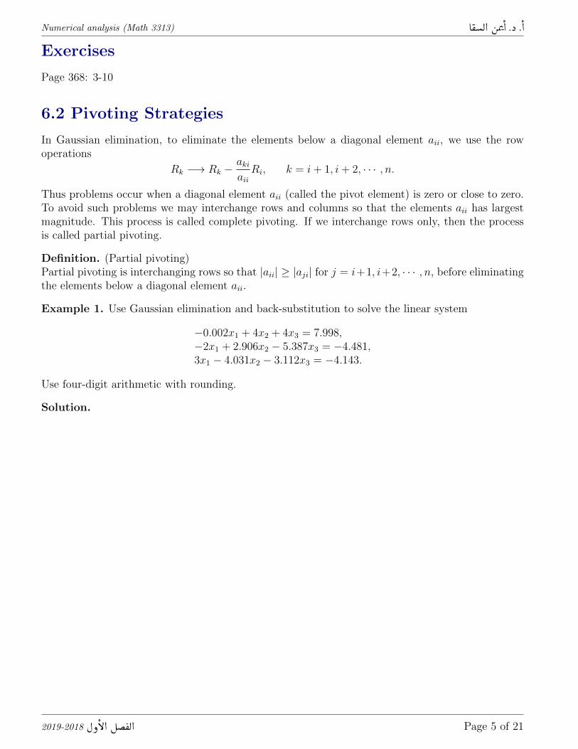
Exercises

Page 368: 3-10

6.2 Pivoting Strategies

In Gaussian elimination, to eliminate the elements below a diagonal element aii, we use the rowoperations

Rk −→ Rk −akiaiiRi, k = i+ 1, i+ 2, · · · , n.

Thus problems occur when a diagonal element aii (called the pivot element) is zero or close to zero.To avoid such problems we may interchange rows and columns so that the elements aii has largestmagnitude. This process is called complete pivoting. If we interchange rows only, then the processis called partial pivoting.

Definition. (Partial pivoting)Partial pivoting is interchanging rows so that |aii| ≥ |aji| for j = i+1, i+2, · · · , n, before eliminatingthe elements below a diagonal element aii.

Example 1. Use Gaussian elimination and back-substitution to solve the linear system

−0.002x1 + 4x2 + 4x3 = 7.998,−2x1 + 2.906x2 − 5.387x3 = −4.481,3x1 − 4.031x2 − 3.112x3 = −4.143.

Use four-digit arithmetic with rounding.

Solution.

2019-2018 Èð B@ É�

®Ë@ of 21


@ . X .

@

Remark. Exact solution: x1 = x2 = x3 = 1.

Example 2. Use Gaussian elimination with partial pivoting and back-substitution to solve the linearsystem

−0.002x1 + 4x2 + 4x3 = 7.998,−2x1 + 2.906x2 − 5.387x3 = −4.481,3x1 − 4.031x2 − 3.112x3 = −4.143.

Use four-digit arithmetic with rounding.

Solution.

2019-2018 Èð B@ É�

®Ë@ of 21


@ . X .

@

Remark. We use pivoting to minimize round-off error and to avoid division by zero .

Gauss-Jordan Method

Gauss-Jordan method is an elimination method to transform the coefficient matrix A of a linearsystem Ax = b to the identity matrix I. As a result of this process, the right-hand side b will betransformed to the solution of the system.

Example. Use Gauss-Jordan method to solve the linear system

2x1 + 2x2 − 2x3 = 2,3x1 + 5x2 + x3 = 5,x1 + 2x2 = 6.

Solution.

2019-2018 Èð B@ É�

®Ë@ of 21


@ . X .

@

Remarks.

(1) Pivoting is normally used with Gauss-Jordan method to preserve arithmetic accuracy.

(2) To solve linear systems with the same coefficient matrix A, but with different right-hand sidesb(1), b(2), · · · , b(k), we apply the row operations to

[A : b(1), b(2), · · · , b(k)]

and reduce it to[U : b(1), b(2), · · · , b(k)].

Then the solutions of the systems are obtained by applying back-substitution to the equivalentsystems

Ux = b(j), j = 1, 2, · · · , k.

Example. Solve the systems Ax = b(i) by Gaussian elimination if

A =

4 −1 32 3 73 6 −1

, b(1) =

001

, b(2) =

−213

.Solution.

2019-2018 Èð B@ É�

®Ë@ of 21


@ . X .

@

Scaling

Scaling is the operation of adjusting the coefficients of a set of equations so that they are all of thesame order of magnitude. To scale a linear system, we divide each equation by the magnitude of thelargest coefficient in each equation. That is, if

A =

a11 a12 · · · a1na21 a22 · · · a2n... · · · ...

...am1 am2 · · · amn

and αj = max {|aj1|, · · · , |ajn|}, then

[A |b ]−scaling− −→

a11α1

a12α1

· · · a1nα1

| b1α1

a21α2

a22α2

· · · a2nα2

| b2α2

...... · · · ... | ...

am1

αm

am2

αm

· · · amn

αm

| bmαm

Example. Consider the system Ax = b, where

A =

200 1 1−1 100 2−50 3 −3

, b =

202101−50

.(a) Solve the system by Gaussian elimination with pivoting.

(b) Solve the system by Gaussian elimination with pivoting and scaling.

Use three digit arithmetic with rounding.

Solution.

2019-2018 Èð B@ É�

®Ë@ of 21


@ . X .

@

2019-2018 Èð B@ É�

®Ë@ of 21


@ . X .

@

Remark. The exact solution of the above example is x1 = x2 = x3 = 1. Thus we see that scalingminimizes round-off error.

Exercises

Page 379: 1-34

6.3 Linear Algebra and Matrix Inversion

In this section we consider some algebra associated with matrices and show how it can be used tosolve problems involving linear systems.

Matrix Inversion

Definition. (1) An n×n matrix A is said to be nonsingular (or invertible) if there exists an n×nmatrix A−1 such that A−1A = AA−1 = I.

(2) The matrix A−1 is called the inverse of A.

(3) A matrix without an inverse is called singular (or noninvertible).

How can we find the inverse of a matrix?

The Gauss-Jordan method can be used to find the inverse of a given matrix A. We augment thegiven matrix A with the identity matrix of the same size. Then we reduce A to the identity matrixI by row operations, performing the same operations on I. As a result I will be transformed to A−1.

[A | I]Gauss-Jordan−−−−→ [I |A−1].

Example. Find the inverse of the matrix A =

2 2 −20 −1 40 2 1

.Solution.

2019-2018 Èð B@ É�

®Ë@ of 21


@ . X .

@

Remark. It is more efficient to use Gaussian elimination instead of Gauss-Jordan method to findA−1. In this case we solve the systems AA−1 = I.

Example. Use Gaussian elimination to find the inverse of the matrix A =

2 2 −20 −1 40 2 1

.Solution.

Remarks.

(1) If A−1 exists, then the solution of the system Ax = b is given by x = A−1b. However this is notthe preferred method for solving Ax = b since it take more time than other methods.

(2) The inverse of a matrix is important for theoretical reasons.

Exercises

Page 390: 5-8, 13-18

2019-2018 Èð B@ É�

®Ë@ of 21


@ . X .

@

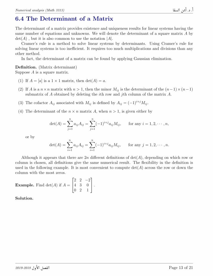
6.4 The Determinant of a Matrix

The determinant of a matrix provides existence and uniqueness results for linear systems having thesame number of equations and unknowns. We will denote the determinant of a square matrix A bydet(A) , but it is also common to use the notation |A|.

Cramer’s rule is a method to solve linear systems by determinants. Using Cramer’s rule forsolving linear systems is too inefficient. It requires too much multiplications and divisions than anyother method.

In fact, the determinant of a matrix can be found by applying Gaussian elimination.

Definition. (Matrix determinant)Suppose A is a square matrix.

(1) If A = [a] is a 1× 1 matrix, then det(A) = a.

(2) If A is a n×n matrix with n > 1, then the minor Mij is the determinant of the (n−1)× (n−1)submatrix of A obtained by deleting the ith row and jth column of the matrix A.

(3) The cofactor Aij associated with Mij is defined by Aij = (−1)i+jMij.

(4) The determinant of the n× n matrix A, when n > 1, is given either by

det(A) =n∑

j=1

aijAij =n∑

j=1

(−1)i+jaijMij, for any i = 1, 2, · · · , n,

or by

det(A) =n∑

i=1

aijAij =n∑

i=1

(−1)i+jaijMij, for any j = 1, 2, · · · , n.

Although it appears that there are 2n different definitions of det(A), depending on which row orcolumn is chosen, all definitions give the same numerical result. The flexibility in the definition isused in the following example. It is most convenient to compute det(A) across the row or down thecolumn with the most zeros.

Example. Find det(A) if A =

2 2 −24 3 00 2 1

.Solution.

2019-2018 Èð B@ É�

®Ë@ of 21


@ . X .

@

Theorem 1. (Properties of the determinant)

(1) If U =

u11 u12 · · · u1n0 u22 · · · u2n...

... · · · unn

is an upper triangular matrix, then det(U) is the product of its

diagonal elements; det(U) = u11u22 · · ·unn.

(2) If L =

l11 0 0 · · · 0l21 l22 0 · · · 0...

...... · · · 0

ln1 ln2 ln3 · · · lnn

is a lower triangular matrix, then det(L) is the product of its

diagonal elements; that is det(L) = l11l22 · · · lnn.

(3) The determinant of a matrix is not changed when a multiple of one row is added to another ofthe matrix.

(4) Interchanging two rows of a matrix changes the sign of its determinant.

(5) Multiplying a row of a matrix by a constant multiplies the value of its determinant by the sameconstant. In other words, if B is obtained from A by applying the row operation Ri −→ cRi,then det(B) = c det(A).

(6) If A and B are n× n matrices, then det(AB) = det(A) det(B).

(7) If A has an inverse, Then det(A−1) =1

det(A).

Example. Find det(A) if A =

2 2 −24 3 00 2 1

.Solution.

2019-2018 Èð B@ É�

®Ë@ of 21


@ . X .

@

The following theorem gives relations between nonsingularity, Gaussian elimination, linear sys-tems, and determinants.

Theorem 2. The following statements are equivalent for any n× n matrix A:

(1) The equation Ax = 0 has the unique solution x = 0.

(2) The system Ax = b has a unique solution for any n−dimensional column vector b.

(3) The matrix A is nonsingular; that is, A−1 exists.

(4) det(A) 6= 0.

(5) Gaussian elimination with row interchanges can be performed on the system Ax = b for anyn−dimensional column vector b.

Exercise

Page 399: 1-8,11-12

6.5 Matrix Factorization

Gaussian elimination is the principal tool in the direct solution of linear systems of equations, so itshould be no surprise that it appears in other guises. In this section we will see that the steps usedto solve a system of the form Ax = b can be used to factor a matrix. The factorization is particularlyuseful when it has the form A = LU , where L is lower triangular matrix and U is an upper triangularmatrix. Although not all matrices have this type of factorization, many matrices that occur in theapplications of numerical analysis have.

To solve the linear system Ax = b, we may solve LUx = b. Define y = Ux. Then LUx = b impliesLy = b. The two systems

Ly = b and Ux = y

are easy to solve. We use forward substitution to solve Ly = b. Then we use back substitution tosolve Ux = y for x which is the solution of Ax = b.

LU Decomposition from Gaussian elimination

Consider a square matrix

A =

a11 a12 · · · a1na21 a22 · · · a2n...

... · · · ...an1 an2 · · · ann

.

We can use Gaussian elimination without row interchanges to write A in the form A = LU , where Lis lower triangular matrix and U is an upper triangular matrix.

Applying a row operation to A is equivalent to multiply A by an elementary matrix; that is amatrix that obtained by applying the same row operation to the identity matrix. To reduce a matrix

to an upper triangular matrix, we need m =n(n− 1)

2row operations; that is we have

A = (EmEm−1 · · ·E2E1)−1U.

2019-2018 Èð B@ É�

®Ë@ of 21


@ . X .

@

The matrix U is the upper triangular matrix we obtain by applying Gaussian elimination to A.The matrix L = (EmEm−1 · · ·E2E1)

−1 is formed from the ratios used in Gaussian elimination; thatis L is given by

L =

1 0 0 · · · 0

a21a11

1 0 · · · 0

a31a11

1 · · · 0

.... . .

an1a11

1

Example. Use Gaussian elimination to find LU decomposition of the matrix A =

2 1 24 4 13 0 2

.Solution.

2019-2018 Èð B@ É�

®Ë@ of 21


@ . X .

@

Permutation Matrices

If we interchange rows during the Gaussian elimination, then LU = A, where A can be obtainedfrom A by interchanging rows. We will now consider the modifications that must be made when rowinterchanges are required. We begin the discussion with the introduction of a class of matrices thatare used to rearrange, or permute, rows of a given matrix.Definition. (Permutation Matrix)An n× n permutation matrix P is a matrix obtained by rearranging the rows of the n× n identitymatrix In.

Example. The matrix P =

1 0 00 0 10 1 0

is a 3× 3 permutation matrix.

Lemma 1. A matrix P is a permutation matrix if and only if each row of P contains all 0 entriesexcept for a single 1, and, in addition, each column of P also contains all 0 entries except for a single1.

At the end of Section 6.4 we saw that for any nonsingular matrix A, the linear system Ax = bcan be solved by Gaussian elimination, with the possibility of row interchanges. If we knew the rowinterchanges that were required to solve the system by Gaussian elimination, we could arrange theoriginal equations in an order that would ensure that no row interchanges are needed. Hence there isa rearrangement of the equations in the system that permits Gaussian elimination to proceed withoutrow interchanges. This implies that for any nonsingular matrix A , a permutation matrix P existsfor which the system

PAx = Pb

can be solved without row interchanges. As a consequence, this matrix PA can be factored intoPA = LU.

The Permuted LU Factorization

A practical method to construct a permuted LU factorization of a given matrix A would proceedas follows. First set up P = L = I as n× n identity matrices. The matrix P will keep track of thepermutations performed during the Gaussian Elimination process, while the entries of L below thediagonal are gradually replaced by the ratios used in Gaussian elimination. Each time two rows ofA are interchanged, the same two rows of P will be interchanged. Moreover, any pair of entries thatboth lie below the diagonal in these same two rows of L must also be interchanged, while entries lyingon and above its diagonal need to stay in their place. At a successful conclusion to the procedure, Awill have been converted into the upper triangular matrix U , while L and P will assume their finalform.Example. Find the permutation matrix P so that PA can be factored into the product LU , where

A =

1 2 −12 4 2−3 −5 6

.

2019-2018 Èð B@ É�

®Ë@ of 21


@ . X .

@

Solution.

2019-2018 Èð B@ É�

®Ë@ of 21


@ . X .

@

Crout Reduction

Crout reduction is the process of writing a matrix A as A = LU , where

U =

1 u12 u13 · · · u1n0 1 u23 · · · u2n...

.... . . . . .

......

......

. . . un−1,n

0 · · · · · · · · · 1

and L =

l11 0 0 · · · 0

l21 l22 0 · · · 0. . .

.... . . 0

ln1 ln2 · · · lnn

.

To find L and U , we multiply L and U and equate the result to A.To illustrate the method let us consider the case n = 3; that is let us consider

A =

a11 a12 a13a21 a22 a23a31 a32 a33

.In this case L and U have the forms

U =

1 u12 u130 1 u230 0 1

and L =

l11 0 0l21 l22 0l31 l32 l33

.Using LU = A, we getl11 l11u12 l11u13

l21 l21u12 + l22 l21u13 + l22u23l31 l31u12 + l32 l31u13 + l32u23 + l33

=

a11 a12 a13a21 a22 a23a31 a32 a33

.This yields 9 equations in 9 unknowns. These equation can be solved as follows:

First ↓: l11 = a11, l21 = a21, l31 = a31.

Second →:l11u12 = a12 ⇒ u12 =

a12l11,

l11u13 = a13 ⇒ u13 =a13l11.

Third ↓: l21u12 + l22 = a22 ⇒ l22 = a22 − l21u12,l31u12 + l32 = a32 ⇒ l32 = a32 − l31u12.

Fourth →: l21u13 + l22u23 = a23 ⇒ u23 =a23 − l21u13

l22.

Fifth ↓: l31u13 + l32u23 + l33 = a23 ⇒ l33 = a33 − l31u13 − l32u23.

Generalizing the above calculations we find

lij = aij −j−1∑k=1

likukj, j = 1, 2, · · · , n; i = j, j + 1, · · · , n.

uij =1

lii

[aij −

i−1∑k=1

likukj

], i = 1, 2, · · · , n− 1; j = i+ 1, i+ 2, · · · , n.

2019-2018 Èð B@ É�

®Ë@ of 21


@ . X .

@

Remarks.

1. In the above two formulas for lij and uij we use the conventionm∑k=1

ck = 0 for m < 1.

2. The above formulas are not independent. We have to use the first formula for j = 1 and thesecond formula for i = 1. Then we apply the formulas for j = 2 and i = 2 and so on.

Example 1. Use Crout reduction to find the LU decomposition of A =

2 1 24 4 13 0 2

.Solution.

2019-2018 Èð B@ É�

®Ë@ of 21


@ . X .

@

Example 2. Use Crout reduction to solve the linear system Ax = b if A =

2 1 24 4 13 0 2

, b =

6−48

.Solution.

Exercise

Page 409: 1-9

2019-2018 Èð B@ É�

®Ë@ of 21

@ .x . ¨ð chapter 6 direct methods for solving linear systemssite.iugaza.edu.ps › asakka ›...

Documents